identifying a reliable connection with the spatial frequency of the patterns. Finally, in order to evaluate the robustness of the estimation of the power low decay, extensive simulations have been performed by adding different levels of noise to the patterns.
Citation: Facchini A, Mocenni C (2013) Recurrence Methods for the Identification of Morphogenetic Patterns. PLoS ONE 8(9): e73686. doi:10.1371/ journal.pone.0073686
Editor:Dennis Salahub, University of Calgary, Canada
ReceivedMay 15, 2013;AcceptedJuly 19, 2013;PublishedSeptember 16, 2013
Copyright:ß2013 Facchini, Mocenni. This is an open-access article distributed under the terms of the Creative Commons Attribution License, which permits unrestricted use, distribution, and reproduction in any medium, provided the original author and source are credited.
Funding:The study is supported by the European Project AWARE, Project N. 226456, Seventh Framework Programme. The funders had no role in study design, data collection and analysis, decision to publish, or preparation of the manuscript.
Competing Interests:The authors have declared that no competing interests exist. * E-mail: [email protected]
Introduction
Morphogenesis is the mechanism for which spatial structures and patterns form spontaneously in biological and biochemical systems. This phenomenon can be explained by assuming that at least two species, an activator and an inhibitor, are interacting in a spatial domain subject to reaction and diffusion processes of different intensities [1]. The striking theory developed by Alan Turing provided a reliable framework for the physical and mathematical understanding and modeling of such complex systems. Although this mechanism is well known and measurable in biology and medicine at different scales, such as molecular and cellular, few studies handle the problem of matching mathematical and numerical models with real measurements. The analysis of these kind of complex spatio-temporal data is complicated by the presence of small disturbancies in the measurements [2], preventing successful application of segmentation techniques for identifying the typical elements in the structures. The presence of noise and quasi periodicities in the measurements introduces further elements of uncertainty and compromises the application of satisfactory analysis in the frequency domain.
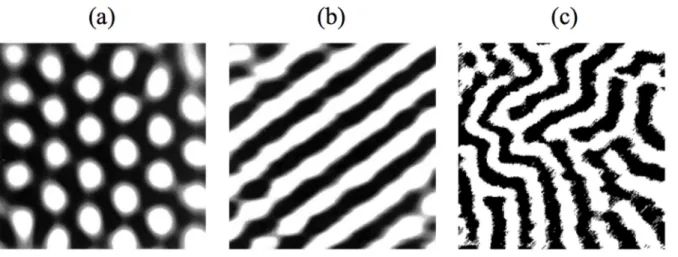
In order to find innovative methodologies for identifying and modelling patterned data arising from biological and biochemical reaction-diffusion processes, we observe that the main feature of such data is the presence of regular structures involving typical patterns (see, for example, spots and stripes of Figure 1. It is straightforward recognizing in these images the quasi periodicity in space, for which a typical element is almost regularly recurrent.
The idea of using methods based on repetitions and recurrences for studying experimental patterns can be related to the concept of
recurrence for complex systems, initially developed by Poincare´ [3]. Indeed, this concept was used by Poincare´ in the field of dynamical systems to solve the three body problem, and by Kac [4] for discrete stochastic systems. For time series, the concept of recurrence was carried out by Eckmann, who introduced the Recurrence Plot (RP) as a visual tool designed to display recurring patterns and to investigate nonstationary patterns [5]. In the field of time series analysis, RPs found a wide range of applications to the analysis of nonstationary phenomena, such as biological systems, speech analysis, financial time series, and earth sciences (see [6] and literature cited therein). The popularity of RPs lies in the fact that their structure is visually appealing and allows for the investigation of high dimensional dynamics by looking at a simple two-dimensional plot. Furthermore, by means of the Recurrence Quantification Analysis (RQA) [7], the RP has been used as a tool for the exploration of bifurcation phenomena and changes in the dynamics when dealing with nonstationary and short time series [8].
microemulsion [13]. Because of the nonlinear features of the models leading to pattern formation, the problem of state space reconstruction and parameter identification is a hard task. State space reconstruction of a spatio-temporal dynamical system has been investigated in lattice dynamical systems [14], while a method for spatial forecasting from single snapshots has been proposed in [15]. Furthermore, in several cases, one has to cope with the problem of understanding the dynamics of a system by using only a limited number of observations.
This work addresses the problem of identifying a correlation between the structure of patterns and model parameters in a prototypical model showing Turing pattern formation. Two numerical experiments are performed by varying the parameters controlling the shape and spatial frequency of the patterns, respectively. Our aim is to establish a functional relationship between the recurrence indicators and the model parameters by means of GRPs and GRQA. We will show that the functional form of the GRQA measures strictly depends on one of the model parameters. The relationship can be used to identify suitable values of the parameters responsible for the generation of patterns, which can be a hard task in experiment design and practical applications. Moreover, this relationship is shown to be robust with respect to noise levels lower than15%.
Results and Discussion
Two numerical experiments have been performed by varying the parametersS andd of the model described in the Materials and Methods section. The parameterScontrols the frequency of the patterns generated, while by varying the diffusion coefficient, d, the patterns are formed or change from spot to labyrinthine. Therefore, by continuously varying these parameters we are able to obtain a set of stationary solutions showing the trajectories from higher to lower pattern frequencies and from spot to labyrinthine structures.
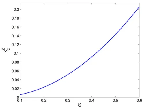
In the first experiment, we set d~0:2, while the spatial frequency of the spot patterns is increased by varying the parameter S in the range ½0:1,0:55. The critical wavenumber k2, which accounts for the spatial frequency of patterns, with respect to parameterSand for fixedd is shown in Figure 2.
In the second experiment, the diffusion coefficientdis varied in the range ½0:02,0:25, while S is kept constant (S~0:3). In this case the spatial frequency of the structures should not change
significantly, while the appearance of the patterns ranges from labyrinthine structures (d~0:02) to spots (d~0:25).
In the following we report the evolution of the recurrence indicators D and RE, described in the Materials and Methods section, with respect toSandd. Furthermore, we will show how the distribution of the diagonal lines P(l) of the RP changes according to the characteristics of the pattern analyzed.
Experiment 1
Figure 3 shows the results of the analysis based on recurrences: panels (a) and (c) report the variableX showing spot patterns for S~0:15 andS~0:47, respectively. Panels (b) and (d) report the corresponding line lengths distributionsP(l). A first inspection of P(l)suggests that the line length decays exponentially (P(l)~e{bl) with different exponents:b~0:71 in the case of smaller spatial frequency (panel (b)) andb~1:02 in the case of higher spatial frequency (panel (d)). In fact, as the frequency increases, the size and distance of the spots decreases, resulting in a smaller number of long diagonal lines. Notice that Lmax~70 for S~0:15 and Lmax~45forS~0:47, whereLmaxis the maximum line length of the RP.
The comparison of D and RE offers a further validation: D dramatically decreases from 53.34 to 18.87, whileREshows only small variations according to the findings (see [10]) that this indicator is more sensitive to changes in the small scale structure of patterns, such as the shape of single patterns, which does not change when increasing the spatial frequency. Furthermore, the strong decrease ofDwithSsuggests a deeper investigation of the relationship of the recurrence indicators fromS.
We then performed an additional experiment by continuously varying S in the interval½0:1,0:55. The results are reported in Movie S1, which is organized as follows: for each S, panel (a) shows the spot patterns; panel (b) reports the values ofD(S)with respect to S; panel (c) reports the computation of the power spectral density of each image showed in panel (a), and, finally, panel (d) reports the values of the main frequencyf0of the patterns (the main frequency has been computed by smoothing the power spectrum in the kx direction and by extracting its maximum value).
Figure 4 shows with greater detail that as S is increased, D decays according the power lawD(S)*S{1=2. This result clearly indicates the existence of a functional relationship between the determinism Dand the parameter S, which controls the spatial frequency of the patterns in the model. The same relationship is Figure 1. Different types of stationary Turing Structures: a) Hexagons b) Stripes c) Labyrinthine.
doi:10.1371/journal.pone.0073686.g001
hardly obtained by computing the power spectral density of the image. Indeed, as one can see in panels (c) and (d) of Figure 5 the
power spectrum is noisy, and an accurate estimation of f0 is difficult. Furthermore,f0(S)does not seem to evolve according to Figure 2. Critical wavenumbersk2
cfor increasing values of parameterS.All the other parameters are fixed:a~16,b~12,d~0:2. doi:10.1371/journal.pone.0073686.g002
Figure 3. Spot patterns for different values of parameterS (panels (a), (c)) and corresponding histograms of line lengthsP(l)
a quadratic function. In conclusion, the determinism represents a good measure for characterizing, both qualitatively and quantita-tively, patterns arising from (potentially unknown) reaction-diffusion models.
Experiment 2
In the second experiment we fix the spatial frequency of the patterns by maintainingSconstant and by varyingdin the range d~½0:02,0:25. This produces patterns with the same spatial frequency, but of different typology. Panels (a) and (c) of Figure 6 show the patterns ford~0:056andd~0:196, respectively, while panels (b) and (d) report the distribution of the line lengthsP(l). Analogously to the first experiment, we look at the distributions of the diagonal linesP(l). Under the new experimental conditions P(l) decays exponentially until the valuel~40 is reached, with similar decay exponents (b~0:41 vs b~0:43). This is not surprising because the spatial frequency of the patterns is very similar, and the line lengths, at least for the first part of the distributions, are not affected by the global shape of the patterns. The same considerations hold forRE. On the contrary, the value of Dis strongly different:D~27:70for the spots (panel (a)) and D~15:00for the labyrinthine structures (panel (c)), reflecting the
fact that, under the point of view of the global appearance of the pattern, the figure reported in panel (c) presents more complex structures, as demonstrated by the fat tail ofP(l)in panel (d). This experiment confirms that D is a powerful measure for the characterization of spatial patterns generated by reaction diffusion models.
Effect of Noise
The methods based on time recurrences have been shown to be robust with respect to noise and measurement errors [6,16], providing suitable tools for analyzing data collected through real experiments.
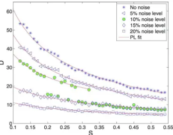
In order to test and eventually find a similar robustness for methods based on spatial recurrences, the spot patterns analyzed in experiment 1 have been corrupted by noise with increasing intensity. Figure 7 reports the evolution of Determinism with respect to the parameterSfor increasing noise levels of5%,10%, 15%and 20%, while the power law decays ofD, obtained by a fitting procedure, are reported in Table 1. The corresponding fitting curves are depicted in the figure by red lines. As the reader can see, the exponent b is consistent with the values obtained without noise and for noise levels of5%and10%. For noise levels Figure 4. Decreasing evolution of the recurrence indicatorDfor increasingS, which is the parameter correlated to the spatial frequency of the patterns.Ddecreases with the power law*S{0:47.
doi:10.1371/journal.pone.0073686.g004
of 15% and 20%, the fitting parameter changes significantly, showing that even if Determinism is still behaving according to a power law, the estimation of the decay exponent b is less reasonable.
Moreover, it is worth noticing that between noise levels of10% and 15%, there exists a threshold separating reasonable and unsatisfactory estimations of the power law relationship. Indeed, the first part of the curve (green circles in Figure 7), corresponding to large size patterns, shows a satisfactory value for b (b~{0:4441), while intermediate-sized patterns, obtained with S~½0:2,0:32, show an interesting intermittency between two different behaviors. Finally, for values ofSgreater thanS~0:32 (small-sized patterns), the decay falls very close to the one corresponding to 15% noise (b~{0:1908). As a possible explanation for this behavior we could consider that as the patterns become smaller and smaller (Sincreasing), the artifacts introduced by noise can deeply modify the structure of the spots or even disrupt them. This fact is also confirmed by the results reported in [10], where it has been shown that Determinism of
spatio-temporal systems decreases in a nonlinear and accelerating way with respect to the increase of noise.
Conclusions
This paper addressed the problem of analyzing morphogenetic patterns emerging from nonlinear systems through physical mechanisms leading to Turing instabilities. The analysis is performed by using a set of recurrence indicators and, in particular, by means of the Generalized Recurrence Plots and Generalized Recurrence Quantification Analysis.
The results clearly show that the method carries out important insights about the structure of patterns and the evolution of such structures under different parametric conditions. Specifically, the main result concerns with the clear identification of the mathematical relationship between the parameter S, related to the spatial frequency of the patterns, and the recurrence indicator D, which accounts for the global appearance of the patterns.
Furthermore, our results will help the experimental scientist in identifying unknown parameters by using the information Figure 5. Snapshot of the last frame of Movie S1.Panel (a): spot distribution forS~0:54. Panel (b): evolution ofDfor increasingSaccording the power law decay discussed in the Results and Discussion section. Panel (c): 2D-FFT showing the power spectral density of the pattern. Panel (d): evolution of the peakf0.
provided by the recurrence measures. Furthermore, when dealing with experiments where a strong sensitivity to the spatial frequency
is present, the proposed method exploits the spatial recurrence properties for retrieving reliable information about the patterns. The obtained results have also been validated by adding noise to the patterns. In this case we found that the power low relationship between the Determinism and the parameterScan be appropri-ately estimated even for noise levels lower than 15%.
Future developments will be devoted to the application of the proposed methodology for the parametric identification of experimental systems, such as bacterial growth and reaction diffusion systems performed in micro-emulsions.
Figure 6. Spot patterns ford= 0.056 (panel (a)) and labyrinthine structures ford= 0.196 (panel (c)).Corresponding histograms of line lengthsP(l)(panels (b) and (d)). By comparing panels (b) and (d) we notice that the values of the exponential decay andREare similar, while the values ofDare considerably different.
doi:10.1371/journal.pone.0073686.g006
Figure 7. Determinism of the patterns for increasing values of parameter S (see also Figure 4) and different noise levels. Specifically, Determinism is reported in the cases of no noise (stars),5% noise (triangles),10%noise (filled green circles),15%noise (diamonds) and20%noise (squares).
doi:10.1371/journal.pone.0073686.g007
Table 1.Fitting parameters of the power lowD~aSBzc between Determinism andSfor different values of noise:5%, 10%,15%and20%.
a b c R2 RMSE
no noise 29.79 20.4508 223.24 0.995 0.78
5% noise level 20.08 20.4891 214.48 0.993 0.72
10% noise level 16.69 20.4441 29.336 0.982 0.66
15% noise level 28.47 20.1908 224.68 0.972 0.51
20% noise level 18.03 20.1666 215.38 0.968 0.29
The last two columns report theR2and the Residuals Mean Square Error (RMSE), respectively.
doi:10.1371/journal.pone.0073686.t001
quite general and hence the principle of a Turing instability can be recovered in other fields, such as heterogeneous catalysis, nonlinear optics, gas discharges, semiconductor devices, and materials irradiated by energetic particles or light. The common denominator of these phenomena is that they can be modeled by reaction-diffusion equations, such as those that naturally describe chemical systems. In all cases, the wavelength of the Turing-type spatial patterns accounts for the balance between the reaction-type mechanisms and the diffusion-like transport processes and is, therefore, intrinsic to the system. Figure 1 shows some of the stationary patterns (also known as Turing Structures, TS) generated by a reaction diffusion system; the type and the shape of TS depend on the values of the model parameters and on the boundary conditions.
Recurrence Based Methods
In this section we provide only basic notions on recurrence methods for spatial data (for a deeper treatment on time series analysis the reader is referred to [6]).
In the case of ad-dimensional data-set, the Recurrence Plot is defined, according to [9], by:
R~ii,~jj~H(e{DD~xx~ii{~xx~jjDD), ð1Þ
where~ii~i1,i2,. . .,idis thed-dimensional coordinate vector and~xx~ii is the associated phase-space vector. This RP, called Generalized Recurrence Plot (GRP), accounts for recurrences between the d-dimensional state vectors and presents a linear manifold of dimensiond for whichR~ii,~jj~1, V~ii~~jj, called the hypersurface of Identity (HOI).
We now consider spatially distributed systems at a certain (fixed) time of their evolution. In the particular case ofd~2, the single variable discretized solution of a two dimensional system can be visualized as an image, i.e. a two-dimensional object composed of scalar values, for which the GRP reads:
Ri1,i2,j1,j2~H(e{DDxi1,i2{xj1,j2DD)ik,jkeNx(:,:)eR: ð2Þ
Each black dot in the GRP represents a spatial recurrence between two pixels, and every pixel is identified by its coordinates (i1,i2), beingi1andi2the row and the column index, respectively. In this case, the recurrence plot is four-dimensional and the HOI is generalized by a two-dimensional identity plane, defined by setting i1~j1andi2~j2.
A visual inspection of the four dimensional RP is possible only by projections in three or two dimensions. Although this is possible
In [10] a different definition of structure of lengthlwas given: instead of looking for two-dimensional patches, we look for the distribution of line segments in the four dimensional GRP. This is done by sampling the patch structures with lines. This can be obtained by looking for the recurrences only in the diagonal direction (k1~k2). With this assumption, the formulation of diagonal line reads:
(1{Ri
1{1,i2{1,j1{1,j2{1)(1{Ri1zl,i2zl,j1zl,j2zl)
P
l{1
k~0Ri1zk,i2zk,j1zk,j2zk:1:
ð4Þ
Focusing on isolated points and lines parallel to the HOI, the recurrence indicators can be generalized and the most important of which are Recurrence Rate RR, Determinism D, and Recurrence EntropyRE.
TheRRis defined as:
RR~ 1
N4
XN
i1,i2,j1,j2
Ri1,i2,j1,j2~ 1 N4
XN
l~1
lP(l), ð5Þ
and represents the fraction of recurrent points with respect to the total number of possible recurrences. It is a density measure of the RP.
The Determinism, defined as:
D~ PN
l~lminlP(l)
PN
l~1lP(l)
, ð6Þ
is the fraction of recurrent points forming diagonal structures with a minimum length lmin with respect to all recurrences. For choosinglminno theoretical guideline is provided and this choice is usually made by means of empirical considerations, such as by taking into account the average size of the patterns or the role of noise in the image.Dprovides a measure of the global appearance of the patterns. For example, highly regular patterns, such as, e.g., periodic structures, will produce high values ofD(more than 50%) since the recurrence points are mainly organized in diagonal lines. On the other side, random or poorly structured patterns are characterized by small values ofD(0.5–1%).
The Recurrence Entropy, defined as:
RE~{ X
N
l~lmin
p(l) logp(l),p(l)~ P(l) PN
l~lminP(l)
is a complexity measure of the distribution of the diagonal lines in the RP.
It refers to the Shannon entropy with respect to the probability of finding a diagonal line of exactly length l. For periodic structures or uncorrelated noise the value is small (0.5–0.8), while for chaotic systems is higher (1.5–2.5). Under the point of view of the pattern,REis related to the small scale structure of the image. The computation of the measures based on the diagonal lines and their distribution provides valuable information about the structure of the RP. For the application of RQA to spatial systems the reader is referred to [9,10].
A Prototypical Model Generating Morphogenetic Patterns
In this paper we considered the model developed by Bard [17], designed to model and reproduce mammalian coat patterns. This model, although simple, describes a nonlinear reaction-diffusion kinetics for simulating Turing patterns. The model generates spots of different complexity, such as rings, and both vertical and horizontal stripes, as well as a variety of labyrinthine structures. The model equations are the following:
LX
Lt ~
S
a(a{XY)z+ 2X
LY
Lt ~
S
a(XY{Y{b)zd+
2Y, ð8Þ
whereSis a constant controlling the spacing of the patterns,dis the ration between the diffusion coefficients of the two speciesX andY,bis the concentration of the enzyme in the domain, anda is a normalization constant. The presence ofbacts as a pattern-formation switch; if b~0, there is a normal stable equilibrium
(X,Y)~(1,a); ifbw0the equilibrium(X,Y)~( a
a{b,a{b)is unstable forawbzpffiffi(
b).
In the last conditions, we observe the formation of spatial patterns whose spatial frequency and shape depend on the diffusion coefficientdand on parameterS.
The formation of the patterns is the result of the propagation of spatial unstable waves, whose wave number rangek2[(k2
1,k22) can be computed as a direct consequence of the instability conditions of the equilibrium point. The verification of the Turing instability conditions is straightforward, as described by Murray [18] (see section 2.3 of volume II).
To the purposes of this work, the model described in equation (8) has been simulated by takinga~16andb~12and varyingS andd. The numerical solutions X and Y are then analyzed by means of the recurrence indicators Determinism and Recurrence Entropy.
Supporting Information
Movie S1 Spot distribution for S~0:56 (panel (a));
Evolution of D for increasing S according the power
law decay discussed in the Results and Discussion section (panel (b)); 2D-FFT showing the power spectral density of the pattern (panel (c)); Evolution of the peakf0
(panel (d)).
(MP4)
Author Contributions
Conceived and designed the experiments: AF CM. Performed the experiments: AF CM. Analyzed the data: AF CM. Contributed reagents/materials/analysis tools: AF CM. Wrote the paper: AF CM.
References
1. Turing A (1952) The chemical basis of morphogenesis. Phil Trans of the Royal Society of London, Series B 237: 37–72.
2. Epstein S (2006) Predicting complex biology with simple chemistry. PNAS 103: 15727–15728.
3. Poincare´ J (1890) Sur la proble`me des trois corps et les e´quation de la dynamique. Acta Math 13: 1–270.
4. Kac M (1947) On the notion of recurrence in discrete stochastic processes. New Bull of the Amer Math Soc 53: 1002–1010.
5. Eckmann J, Kamphorst S, Ruelle D (1987) Recurrence plot of dynamical systems. Europhys Lett 5: 973–977.
6. Marwan N, Romano M, Thiel M, Kurths J (2007) Recurrence plots for the analysis of complex systems. Phys Rep 438: 237–329.
7. Webber C, Zbilut J (1994) Dynamical assessment of physiological systems and states using recurrence plot strategies. Appl Physiol 76: 965–973.
8. Trulla L, Giuliani A, Zbilut J,Webber C, jr (1996) Recurrence quantification analysis of the logistic equation with transients. Phys Lett A 223: 255–260. 9. Marwan N, Kurths J, Saparin P (2007) Generalised recurrence plots analysis for
spatial data. Phys Lett A 360: 545–555.
10. Facchini A, Mocenni C, Vicino A (2009) Generalized recurrence plots for the analysis of images from spatially distributed systems. Physica D 238: 162–169.
11. Mocenni C, Facchini A, Vicino A (2011) Comparison of recurrence quantification methods for the analysis of temporal and spatial chaos. Math and Comp Mod 53: 1535–1545.
12. Mocenni C, Facchini A, Vicino A (2010) Identifying the dynamics of complex spatio-temporal systems by spatial recurrence properties. PNAS 107: 8097– 8102.
13. Facchini A, Rossi F, Mocenni C (2009) Spatial recurrence strategies reveal different routes to turing pattern formation in chemical systems. Phys Lett A 373: 4266–4272.
14. Guo L, Billings S (2007) State-space reconstruction and spatio-temporal prediction of lattice dynamical systems. IEEE Trans on Autom Control 52: 622–632.
15. Marcos-Nikolaus P, Martin-Gonza´lez J, Sole´ R (2002) Spatial forecasting: Detecting determinism from single snapshots. Int J of Bif and Chaos 12: 369– 376.
16. Zbilut J, Giuliani A, Webber C, jr (1998) Detecting deterministic signals in exceptionally noisy environments using cross-recurrence quantification. Phys Lett A 246: 122–128.
17. Bard J (1981) A model for generating aspects of zebra and other mammalian coat patterns. Phys Lett A 93: 363–385.
18. Murray J (2002) Mathematical Biology. Springer-Verlag (Berlin).