Interannual variability of tropospheric composition: the influence of changes in emissions, meteorology and clouds

(1)

ACPD

9, 14023–14057, 2009

Drivers of tropospheric interannual variability

A. Voulgarakis et al.

Title Page

Abstract Introduction

Conclusions References

Tables Figures

◭ ◮

Back Close

Full Screen / Esc

Printer-friendly Version

Interactive Discussion Atmos. Chem. Phys. Discuss., 9, 14023–14057, 2009

www.atmos-chem-phys-discuss.net/9/14023/2009/ © Author(s) 2009. This work is distributed under the Creative Commons Attribution 3.0 License.

Atmospheric Chemistry and Physics Discussions

This discussion paper is/has been under review for the journalAtmospheric Chemistry

and Physics (ACP). Please refer to the corresponding final paper inACPif available.

Interannual variability of tropospheric

composition: the influence of changes in

emissions, meteorology and clouds

A. Voulgarakis1,*, N. H. Savage2, P. Braesicke1, O. Wild3, G. D. Carver1, and J. A. Pyle1

1

Centre for Atmospheric Science, University of Cambridge, UK

2

Met Office, Exeter, UK

3

Lancaster Environment Centre, University of Lancaster, UK

*

now at: NASA/GISS and Columbia University Center for Climate Systems Research, New York, USA

Received: 15 June 2009 – Accepted: 19 June 2009 – Published: 26 June 2009

Correspondence to: A. Voulgarakis (avoulgarakis@giss.nasa.gov)

(2)

ACPD

9, 14023–14057, 2009

Title Page

Tables Figures

◭ ◮

Back Close

Full Screen / Esc

Interactive Discussion

Abstract

We have run a chemistry transport model (CTM) to systematically examine the drivers of interannual variability of tropospheric composition. On a global scale, changing me-teorology (winds, temperatures, humidity and clouds) is found to be the most important factor driving interannual variability of NO2 and ozone on the timescales considered.

5

The strong influence of emissions is largely confined to areas where intense biomass burning events occur. For CO, interannual variability is almost solely driven by emission changes, while for OH meteorology dominates, with the radiative influence of clouds being a very strong contributor. Through a simple attribution analysis we conclude that changing cloudiness drives 25% of the interannual variability of OH over Europe by

af-10

fecting shortwave radiation. Over Indonesia this figure is as high as 71%. Changes in cloudiness contribute a small but non-negligible amount (up to 6%) to the interannual variability of ozone over Europe and Indonesia. This suggests that future assessments of trends in tropospheric oxidizing capacity should account for interannual variability in cloudiness, a factor neglected in many previous studies. The approach followed in the

15

current study can help explain observed tropospheric variability, such as the increases in ozone concentrations over Europe in 1998.

1 Introduction

Tropospheric trace gases play an important role in the Earth system, influencing climate (CH₄, ozone) and determining air quality (ozone, NO_x, volatile organic compounds).

20

Their concentrations vary on a vast range of timescales, and characterising this vari-ability is a major challenge. In particular, understanding what drives the interannual variability (IAV) of annual and seasonal mean concentrations of oxidants is important for explaining the observed trends of tropospheric composition.

Recent model studies have examined the drivers of interannual variability of

tropo-25

(3)

ACPD

9, 14023–14057, 2009

Title Page

Tables Figures

◭ ◮

Back Close

Full Screen / Esc

Interactive Discussion 2006), CO (e.g. Szopa et al., 2007) and NO₂ (e.g. Uno et al., 2007; Savage et al.,

2008), reaching to a variety of useful conclusions. However, a systematic study a) in-volving more than one interdependent species, b) focusing on global as well as regional scales, and c) investigating the role of clouds separately in addition to meteorology and emissions, has not been presented so far. Especially the radiative effect of clouds on

5

chemistry (through photolysis) has commonly been neglected as a driver of either IAV or trends in previous studies.

One factor that can affect tropospheric composition significantly is changing emis-sions from anthropogenic sources. These have changed significantly during recent times in many parts of the globe: in East Asia, rapid industrial development has caused

10

a dramatic increase of pollution (Richter et al., 2005), while in Western Europe, indus-trial/transport emissions have slowly decreased during the 1990s due to control strate-gies (Fowler et al., 2001). Changes in biomass burning emissions (NOx, CO, aerosols)

from year to year can also a_ffect tropospheric composition. An example is the fluctua-tions in wildfire-driven emissions over the Maritime Continent, depending on whether a

15

year is characterized by El Ni ño or La Ni ña conditions (Hauglustaine et al., 1999). Meteorology is also known to be very important in driving tropospheric composition IAV, but the extent of this influence is debated. Extraordinary meteorological condi-tions, like strong El Ni ño events (e.g. in 1997–1998) can lead to large year-to-year changes, with O₃ increases over the Western Pacific and decreases over its eastern

20

parts (Chandra et al., 1998; Sudo and Takahashi, 2001; Doherty et al., 2006). There is evidence that El Ni ˜no also has an impact on the amount of stratospheric ozone en-tering the troposphere through stratosphere-troposphere exchange (STE) (Zeng and Pyle, 2005).

Apart from the strongly anomalous situations related to El Ni ˜no, meteorology can

25

(4)

ACPD

9, 14023–14057, 2009

Title Page

Tables Figures

◭ ◮

Back Close

Full Screen / Esc

Interactive Discussion et al., 2003; Pfister et al., 2004; Derwent et al., 2004; Auvray and Bey, 2005). On the

other hand, European pollution can impact either cleaner areas like the Atlantic and Northern Africa (Duncan and Bey, 2004) or North America during anomalous transport events (Li et al., 2002). Transpacific transport can also be very important, especially during El Ni ˜no years when Asian emissions can impact clean oceanic regions

signif-5

icantly, or even reach North America depending on the local meteorology (Liu et al., 2005). All the above midlatitude processes show significant interannual variability.

We focus here on the 1996–2000 period to investigate what the most important drivers of IAV are. Similarly short periods have been used to examine trends in re-cent studies (e.g. Richter et al., 2005). However, the focus of the current study is not

10

specifically to assess the trends during 1996–2000, but to extract useful conclusions on the factors affecting IAV by applying a method based on Savage et al. (2008).

In Sect. 2 we present the basic model features and the experimental set-up, as well as show that the model reasonably captures the regions of significant variability in pollution. Section 3 analyzes the drivers of IAV of global NO2and ozone columns, while

15

Sect. 4 quantitatively assesses the influence of emissions, meteorology and clouds on ozone, CO and OH. Finally, the conclusions are included in Sect. 5.

2 Model set-up and validation of its ability to capture interannual variability

The model used for the experiments is the updated version of the p-TOMCAT tropo-spheric CTM described in Voulgarakis et al. (2009a). A detailed description of the

20

ozone budget as calculated in the model is described in Voulgarakis et al. (2009b). The horizontal resolution is 2.8◦×2.8◦ and there are 31 vertical levels extending from the surface to 10 hPa. Tropospheric chemistry for 63 trace species is simulated with the ASAD chemistry package (Carver et al., 1997), and photolysis rates are calculated using the Fast-JX photolysis scheme (Wild et al., 2000). Six-hourly meteorological data

25

(5)

ACPD

9, 14023–14057, 2009

Title Page

Tables Figures

◭ ◮

Back Close

Full Screen / Esc

Interactive Discussion Annually and monthly-varying emissions for industry, transport, shipping and

biomass burning come from the RETRO emissions database (Schultz, 2007). Biogenic emissions are taken from M ¨uller (1992) and Lathi `ere et al. (2006). Lightning emissions of NOx are based on the parameterization of Price and Rind (1994) as implemented

by Stockwell et al. (1999). The average lightning emission for the 1996–2000 period

5

is 3.9 Tg(N)yr−1. We use a fixed global annual 3-D field for methane produced from an earlier long-term integration (global burden: 4760 Tg methane). Year-to-year vari-ations in global annual total emissions for each species are shown in Table 1. For most, the highest global emission rates occurred in 1997–1998. As noted in Sect. 1, these two years were characterized by intense wildfire events, which influenced global

10

tropospheric chemistry for many months.

The analysis is based on the results of three model integrations from 1996 to 2000: a) BASE, in which all variables vary from year to year, b) EmFix, in which the surface emissions of all species vary seasonally but not interannually (fixed at 1996 values) and c) MetFix, in which the 1996 meteorology (temperatures, winds, humidity and clouds)

15

is repeated for each year (still varying 6-hourly). The model was run from June 1995 to December 1995 for spin-up. In Table 2 we summarise these runs. CldFix, a run like BASE but with clouds only fixed at 1996 values, is analyzed in Sect. 4.

A detailed evaluation, presented in Voulgarakis et al. (2009a), showed that the model is capable of capturing ozone and CO seasonal cycles well, and that the

concentra-20

tions of these tracers at various sites compare well with observations. Notable under-estimates were found in the Northern Hemisphere for surface CO and overunder-estimates in the upper troposphere for ozone. These features are relatively common in present-day global models (Shindell et al., 2006; Stevenson et al., 2006).

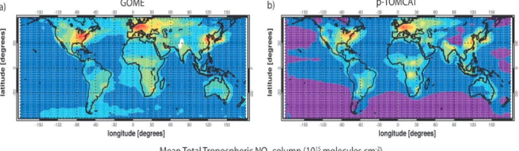
In Fig. 1 we present a comparison of global modelled NO2to observations from the

25

(6)

ACPD

9, 14023–14057, 2009

Title Page

Tables Figures

◭ ◮

Back Close

Full Screen / Esc

Interactive Discussion Savage et al. (2008), and the annual averaging helps to remove random errors in the

measurements.

The model generally captures the distribution of NO2 tropospheric column maxima

around the globe quite well, and this is also true on a seasonal basis (not shown). The model underestimates total NO2 in the Northern Hemisphere, especially over

in-5

dustrialized regions (Northeast America, Western Europe, East Asia), suggesting that the NO₂ lifetime may be too short in the model. However, there is an overestimation of the maxima related to biomass burning in the tropics (Indonesia, Central Africa). Over South America and Central/Southern Africa the observed columns are more spa-tially widespread than those in the model runs, where maxima occur closer to source

10

regions. This negative model bias over industrialized regions and positive bias over biomass burning regions are also evident for most of the models involved in the inter-comparison reported by van Noije et al. (2006). They did not reach to a clear conclusion as to what causes these discrepancies.

The absolute standard deviations of the NO2 column (Fig. 1c and d) show that

re-15

gions of strong IAV are captured reasonably well, but the amplitude of year-to-year variations is underestimated by the model over northern hemispheric industrialized re-gions. For the areas where strong biomass burning events occur IAV is overestimated. These differences between measured and modelled standard deviations could be re-lated to uncertainties in the column retrievals or to uncertainties in the modelled IAV.

20

Examining the standard deviation normalized to the 5-year mean (not shown), we find that underestimated variability over industrialized regions shown in Fig. 1 is not caused by the underestimation of NO₂ columns. Possible reasons for these discrepancies in-clude a) lack of IAV in aerosol concentrations driving NO2 loss in the model and b)

no representation of year-to-year variations in methane and stratospheric ozone in the

25

runs analyzed for the current study.

(7)

ACPD

9, 14023–14057, 2009

Title Page

Tables Figures

◭ ◮

Back Close

Full Screen / Esc

3 Emissions and meteorology: their influence on NO₂ and ozone interannual variability

3.1 Tropospheric NO₂column interannual variability

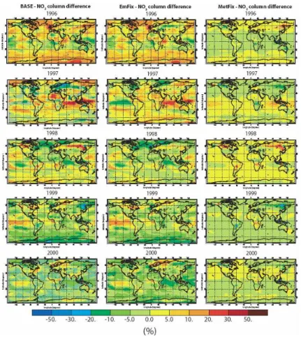
Figure 2 shows the 1996–2000 differences from the 5-year mean of tropospheric NO2

columns for all individual years. The BASE run describes the overall IAV. In the

5

idealized case that these differences were entirely driven by emission (meteorology) changes, the values on the plots for the EmFix (MetFix) run would all be zero, while the ones for the MetFix (EmFix) run would look identical to the ones for BASE. We focus on percentage differences, as they better highlight the effect of emissions and meteorology both over polluted and un-polluted regions. Recall that in Fig. 1 we had

10

shown the average NO₂columns, and its standard deviations, in concentration units. It is clear from Fig. 2 that the BASE and EmFix differences look very similar for cor-responding years, while the ones for MetFix differ significantly, with deviations from the 5-year mean being generally closer to 0%. This indicates that IAV in meteorology is far more important as a driver for changes in NO₂abundances than emissions over most

15

of the globe on these timescales. The only regions where IAV is captured with fixed me-teorology are associated with important biomass burning events. The 1997 and 1998 events in Indonesia (Hauglustaine et al., 1999) and Siberia/Canada (Spichtinger et al., 2004) correspondingly cause large differences from the 5-year mean (up to+240% in Indonesia and +100% in Siberia) which dominate the variability over these regions.

20

To a lesser extent, fires over Central Africa/Amazonia (mainly 1998) and the Iberian peninsula (2000) appear to drive much of NO2 IAV over these areas. As discussed

in Sect. 2, the effect of fires over tropical regions may be overestimated in the model, but the dominant role of emissions in controlling the variability is expected to be repre-sented well.

25

Changes in meteorology drive the IAV of NO2 in a number of regions around the

(8)

ACPD

9, 14023–14057, 2009

Title Page

Tables Figures

◭ ◮

Back Close

Full Screen / Esc

Interactive Discussion (MetFix plot for 1997). When these emissions are not taken into account, a

reduc-tion in the NO₂ maximum over Borneo and Sumatra is seen. Apart from the biomass burning effect, the decrease is also enhanced by the reduction in lightning NOx due

to suppressed convection. But there are still large increases in the columns in the surrounding areas (Indian Ocean, Central West Pacific) captured mainly by

meteoro-5

logical IAV. The export of pollution from Indonesia during late 1997 occurred primarily towards these regions (Duncan et al., 2003). NO2has a short lifetime, so not much of

it is transported far, but peroxyacetyl nitrate (PAN), a major reservoir of NO_x, can be transported and release NO2at a large distance from the source region.

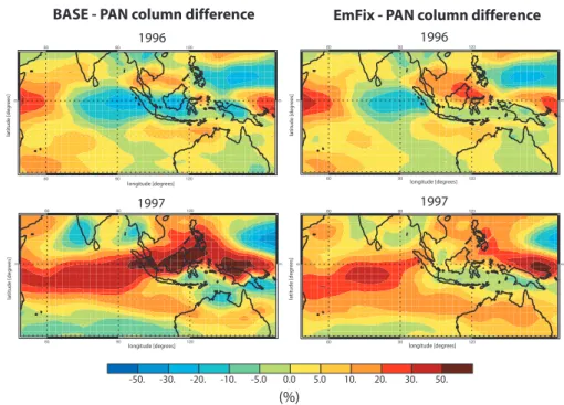
Figure 3 shows PAN tropospheric column differences from the 5-year mean for 1997

10

and 1996. From the BASE run, it is clear that PAN increases in 1997 over the Mar-itime Continent when compared to 1996. When emissions are fixed at 1996 values (EmFix) (1996 was not an anomalous year for biomass burning in Indonesia) PAN still increases over surrounding regions. The anomalous circulation patterns caused by El Ni ˜no (mainly the strong surface-level divergence centred around Indonesia) increases

15

the export of pollution significantly and explains the large increases of PAN, and sub-sequently NO₂, over the Indian Ocean and the Central Western Pacific.

El Ni ˜no-associated dryness, another meteorological factor (Chandra et al., 1998), could also have played a role in increasing NO2 columns, as a reduced abundance of

OH would increase the lifetime of NO_x. However, as shown later, 1997 was a year with

20

high OH levels over Indonesia due to reduced cloud cover, so dryness cannot have been the main driving factor. Decreased wet deposition of HNO3, a loss process for

NO_x, will also play some role in boosting the positive signals over the Indian Ocean and Western Pacific.

The opposite effect during 1997 is seen for the NO2column over the Central/Eastern

25

Pacific and is almost entirely driven by meteorology. This is consistent with Sudo and Takahashi (2001). Higher humidity and HNO3 wet deposition are expected to be the

main reasons for this feature.

(9)

ACPD

9, 14023–14057, 2009

Title Page

Tables Figures

◭ ◮

Back Close

Full Screen / Esc

Interactive Discussion column deviations from the 5-year mean include: a) large increases in NO₂ columns

over the British Isles in 1996, as also seen by Savage et al. (2008), b) low NO2columns

offthe east coast of North America in 1996, and c) increased NO2columns offthe west

coast of Central Africa in 1999–2000.

In all these cases, the deviations from the 5-year mean seen in the EmFix case

5

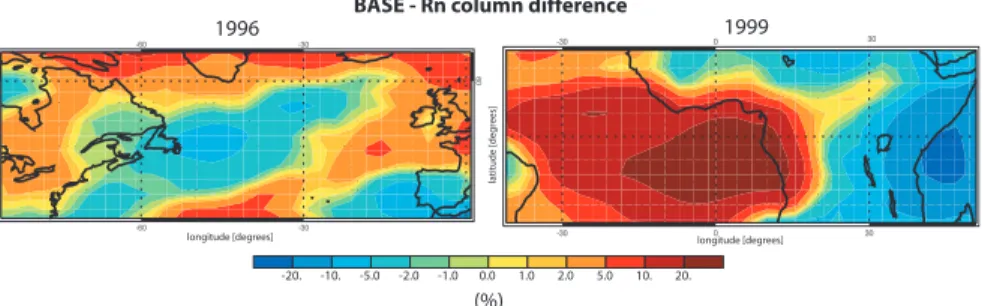
are associated only with changes in meteorology. They can be related to increased lightning activity (especially in the tropics), humidity, cloud optical depths or anomalous transport processes in the corresponding years. The influence of transport can be isolated by looking at the differences from the 5-year mean of the radon tracer, based on the method described by Jacob et al. (1997). Radon has a short lifetime of around

10

5.5 days, is emitted predominantly over land and its tropospheric distribution depends strongly on horizontal and vertical transport. Figure 4 shows the difference from the 5-year mean of its abundances over the British Isles and Northwest Atlantic (1996) and over West Central Africa (1999). Both for the midlatitude and the tropical areas it is clear that the minimum and maximum radon deviations are strongly correlated

15

with the features found for NO2 over the same areas. Transport of NO2 itself or of

reservoir species (PAN, HNO₃) away from sources is the most important factor driving these features. The deviations over the British Isles and offthe east coast of North America in 1996 are associated with the negative phase of the NAO leading to a) less storm/frontal activity and thus less smearing of NO₂features and b) less e_ffective

long-20

range transport of plumes (Creilson et al., 2003) across the Atlantic.

Note that the changes in meteorology are almost entirely responsible for year-to-year NO₂ variability over the oceans, while over land the emission changes also appear to play some role (though in general smaller than that of meteorological changes). The fact that the oceans are areas with low NO2 abundance (see Fig. 1) does not

dimin-25

ish the importance of this conclusion, since in NO_x-limited environments even small changes in NO2 concentrations can have a significant effect on other tracer budgets

(10)

ACPD

9, 14023–14057, 2009

Title Page

Tables Figures

◭ ◮

Back Close

Full Screen / Esc

Interactive Discussion over the oceans.

3.2 Tropospheric ozone column interannual variability

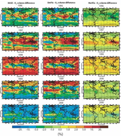
Figure 5 shows the di_fferences between each year’s tropospheric ozone columns and the 5-year mean. The maximum differences for ozone are smaller than for NO2

(max-imum+36% over Indonesia in 1997 and around+20% over northern high latitudes in

5

1998). However, the various meteorological and emission effects are still important and dominate large parts of the globe due to the longer lifetime of ozone compared to NO2. A common feature of Fig. 2 and Fig. 5 is that the BASE and EmFix plots

again look similar, implying that changing meteorology was the most important driver of tropospheric ozone IAV during this 5-year period.

10

The ozone increases in the tropics in 1997 are driven both by the intense biomass burning events over Indonesia (increase of precursors) and by the favourable meteoro-logical situation related to El Ni ˜no: suppressed convection, downward motion and dry-ness favour both the downward transport of ozone-rich upper tropospheric air through-out the troposphere and decreased ozone loss by the O1D+H₂O reaction, over a large

15

area centred around Indonesia. The effects on NOx mentioned in the previous section

are also important, since NO and NO2are major ozone precursors. The ozone

pollu-tion resulting from the wildfires was transported to large distances from the sources. The only tropical area where ozone decreased in 1997 is the Central/Eastern Pacific where conditions are opposite to those found over the Western Pacific. When fixing

20

meteorology to 1996 values (MetFix), this feature disappears completely and increases are found in almost all tropical areas, excluding Central Africa, possibly due to lower than average biomass burning emissions in 1997. However, the positive differences with MetFix are smaller in magnitude than with the other two runs; the only region where they are larger than+5% is over and around Indonesia. Thus, while the IAV in

25

emissions alone would cause ozone increases in tropical areas, it is the meteorology, related to El Ni ˜no, which makes this more than a regional feature.

(11)

ACPD

9, 14023–14057, 2009

Title Page

Tables Figures

◭ ◮

Back Close

Full Screen / Esc

Interactive Discussion the extratropical areas, almost symmetrically centred around the tropics, where

neg-ative differences occur. The large boreal fires which occurred during that year and, to a smaller extent, the high fire activity in South America caused large increases in the amount of ozone precursors in the troposphere, partly causing the increases in extratropical ozone in this year. Also, the impact of tropical pollution produced in 1997

5

is expected to have a signal in the extratropics for several months, especially through the long-range transport of long-lived precursors (e.g., CO, see Duncan et al. (2003)). However, with emissions at 1996 values (EmFix), all the features of the BASE plot for 1998 are preserved, with just a small reduction in the deviations. In contrast, with fixed meteorology (MetFix), smaller, almost globally distributed deviations from the

5-10

year mean are found for this year, with maxima of 2–5% located around the main biomass burning regions. Anomalous emissions only cause a small fraction of this year’s anomaly seen in the extratropics.

The fact that the large extratropical positive deviations from the 5-year mean in 1998 are ubiquitous could indicate that long-range transport from other mid-latitude

anthro-15

pogenically polluted areas may not be the cause of the extratropical ozone increases. High horizontal wind speeds, transporting ozone and precursors to unpolluted regions, would also have caused reductions of tracer concentrations over the polluted areas. But large increases are seen in the BASE and EmFix runs even for the southern ex-tratropics where pollution sources are much less than at northern mid/high latitudes,

20

suggesting that long-range transport within the troposphere is not the main reason for ozone increases. Zeng and Pyle (2005) found that 1998 was a year of very high STE in the extratropics associated with high SST anomalies in the Pacific (El Ni ˜no) a few months earlier. This transport-related process which is a_ffected directly when fixing meteorology to 1996 is more likely to have caused the large positive signal.

25

By examining the IAV of tropopause heights around the globe for the 1996–2000 period we note that the main features of Fig. 5 are not driven by changes in the total mass of air included in the calculated tropospheric columns.

(12)

meteorol-ACPD

9, 14023–14057, 2009

Title Page

Tables Figures

◭ ◮

Back Close

Full Screen / Esc

Interactive Discussion ogy is through changes in horizontal and vertical transport. However, other

meteorolog-ical variables may have an influence, and the most important of these are humidity and cloud optical depth. Water vapor can increase loss of ozone (via O1D+H2O) but can

also enhance the production of peroxy radicals which drive ozone production. How-ever, there were no large hemispheric-scale increases in water vapour in 1998 in the

5

model. We therefore examine the role of clouds in determining IAV of ozone in the next section.

4 Quantitative analysis of the role of emissions, meteorology and clouds

Clouds play an important role in altering photochemical processes by modifying solar radiation throughout the tropospheric column. To our knowledge, there have been no

10

previous studies assessing the role of clouds in the IAV of global tropospheric compo-sition. Here we separate the shortwave radiative effect of clouds from other aspects of meteorological variability by conducting an additional model run. In this run, CldFix, 6-hourly varying 3-D cloud optical depths for 1996 are used throughout the 1996–2000 period; everything else varies as in BASE. Note that “clouds” are a subset of

“mete-15

orology” in the current approach, meaning that in the case that meteorology is fixed to 1996 values (MetFix), clouds are kept fixed as well. Deviations of the tracer abun-dances from the 5-year mean are compared to those seen when fixing the meteorology or the emissions to 1996 conditions.

4.1 Analysis of global ozone IAV drivers

20

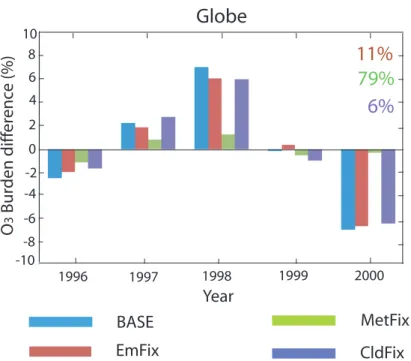
Figure 6 shows the difference in each year’s ozone burden from the 5-year mean. It also shows the percentage of variability which is explained by each one of the factors separately, calculated using a simplified attribution approach based on Szopa et al. (2007). The 5-year anomalies for each run were averaged and then divided by the average anomaly for the BASE run in order to determine by how much the variability is

(13)

ACPD

9, 14023–14057, 2009

Title Page Abstract Introduction Conclusions References Tables Figures ◭ ◮ ◭ ◮ Back Close

Full Screen / Esc

Interactive Discussion reduced when each field is fixed at 1996 values. By subtracting this percentage from

100, the variability explained by each individual factor can be quantified. The equation used is the following:

P ₌        1− 1 N N X

i₌0

X(i)S −X(i)S 1 N N X

i₌0

X(i)B−X(i)B       

×100 (1)

whereP _{is the percentage shown on the plots,} X₍i₎_S _{represents the anomalies from}

5

the 5-year mean for each year in the sensitivity runs (EmFix, MetFix, CldFix), andX₍i₎_B

is the same variable but for the BASE run. N _{is the number of years considered (5 in}

this study).

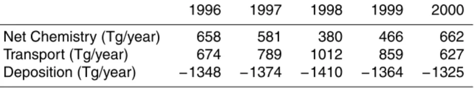
Figure 6 shows a strong peak in the global ozone burden (+7% in 1998) associated with the 1997–1998 El Ni ˜no event. Table 3 shows the global annual budget terms

10

for 1996–2000 as calculated in the BASE run. It is clear that the increased global tropospheric ozone abundances found in the 1997–1999 period are strongly related to increases in STE. Net chemical production is lower than average during these years and the deposition rate is larger, so changes in these terms are unlikely to have driven the ozone burden increases we find here.

15

Changes in meteorology have a stronger impact on global ozone than changes in emissions. The variability in the MetFix run is very small, and shows only a small in-crease in 1998 reflecting the intense wildfires. Meteorology drives almost 80% percent of the IAV of ozone on a global scale.

Clouds exert a smaller but non-negligible influence in the IAV of the ozone burdens.

20

Globally they are responsible for 6% of the variability, which is around 8% of the total influence of changes in meteorology.

(14)

ACPD

9, 14023–14057, 2009

Title Page

Tables Figures

◭ ◮

Back Close

Full Screen / Esc

4.2 Regional scale analysis: Europe and Indonesia

We focus here on Europe and Indonesia as important examples of the northern ex-tratropics and the tropics in order to examine how similar the responses of ozone, CO and OH are in these regions to year-to-year changes in emissions, meteorology and clouds.

5

4.2.1 Tropospheric ozone IAV

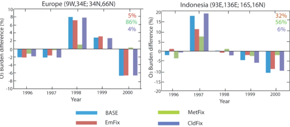
Figure 7 shows that there is a maximum in O3burden over Europe in 1998 followed by

a relative decline in 1999 and, especially, 2000. Meteorology is responsible for 86% of this variability while emissions changes are less important (5% compared to 8% generally in the northern extratropics). Cloud changes drive 4% of the European O3

10

IAV. Over Indonesia, emissions drive a significant part of O₃IAV (32%).

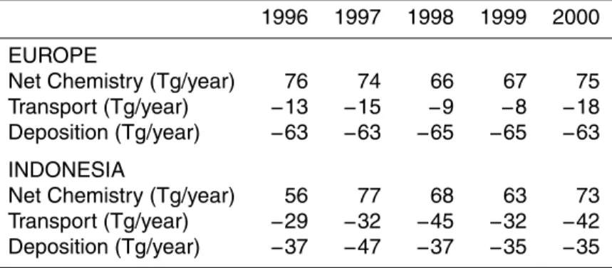
Table 4 shows the regional ozone budget terms for the BASE run over Europe and In-donesia. Europe is a net exporter of ozone for all the years of study (−8 to−18 Tg/yr), and and we find a decrease in the net export of ozone from Europe in 1998–1999 (around 30% less than average) which may reflect increased import or decreased

ex-15

port. Net chemistry (production minus loss) was lower than average during the same years and deposition was higher due to higher ozone concentrations, so the ozone peak is attributed to the decreased net export term. Decreased net export may be a re-sult of both/either decreased net chemistry and/or the dominance of transport regimes which do not favor export. Similarly, the ozone burden decrease over Europe in 2000

20

(La Ni ˜na period since 1999) can be attributed to changes in net transport of ozone from the European region.

With the approach taken in this study, we are able to attribute the features of the tropospheric ozone distribution to a variety of influences. Confidence in the approach is given by the fact that the BASE model is able to capture major features of the

ob-25

(15)

ACPD

9, 14023–14057, 2009

Title Page

Tables Figures

◭ ◮

Back Close

Full Screen / Esc

Interactive Discussion revealed by measurements and as calculated by the model. Zugspitze is considered to

be representative of Central Europe for background atmospheric studies (e.g. Kaiser et al., 2007). Clearly the model captures the important ozone increases from late 1997 to mid 1999, and the much lower than average values in 2000.

Over Indonesia, also a net exporter of ozone, the 1997 ozone burden maximum is

5

caused by increased net chemistry but also by slightly lower than average net export from the region. This is most likely caused by subsidence of stratospheric ozone-rich air causing increased import of ozone. Horizontal transport to Indonesia within the troposphere was lower than average in 1997 due to strong low-level divergence. In 2000, the minimum ozone burden relates to the transport term being around 20%

10

lower than average, meaning higher than average net export.

4.2.2 Tropospheric CO and OH IAV

Figure 9 shows the CO and OH results of the four runs (BASE, EmFix, MetFix and CldFix) for Europe and Indonesia. For CO, clouds make a minor contribution, espe-cially over Indonesia where only 1% of the IAV is explained by changes in cloudiness.

15

Changes in meteorology are far less important than they are for ozone. Year-to-year variations in emissions explain 92% of the IAV of CO over Indonesia and even over Europe, where biomass burning is not nearly so intense, this figure is as high as 82%. These results contrast with those of Szopa et al. (2007), who found that in the tropics meteorology is the main reason driving CO IAV, while in the extratropics changes in

20

emissions and meteorology are equally important. Differences in chemical schemes, such as in the secondary production of CO from hydrocarbon oxidation, may partly explain these different results. As noted in Sect. 2, p-TOMCAT overestimates pollution over Indonesia during the period of this study, suggesting that the effects on tropical IAV may be exaggerated. However, we do not expect that the main IAV signal would

25

change with the use of lower emissions.

(16)

ex-ACPD

9, 14023–14057, 2009

Title Page

Tables Figures

◭ ◮

Back Close

Full Screen / Esc

Interactive Discussion pected to be greatest. As shown by Voulgarakis et al. (2009b) and other previous

stud-ies, above and below-cloud modification of radiation is more important than in-cloud effects for OH. For Europe, we present the results for summer (June-July-August), as this is also the season with the greatest solar radiation, when the impact of clouds on OH concentrations is highest. The figures show that when meteorology does not

5

vary, almost none of the OH IAV is reproduced. This is consistent with Dentener et al. (2003), who found that IAV in OH is driven more strongly by meteorology than by sur-face emissions changes. It is clear that clouds are a very important component of this OH variability in the lower troposphere. 71% of the year-to-year variations in OH over Indonesia are caused by changes in cloudiness. Over Europe the figure is smaller

10

(25%) but still important. Thus, radiative cloud e_ffects should not be ignored when studying the IAV of the tropospheric oxidizing capacity, especially since OH changes affect methane, a gas of major climate importance.

An OH minimum in 1998 (−4%) over Europe can be partly explained by changes in cloudiness: it is less pronounced when fixing clouds and cloud optical depths are

15

indeed lower than average in 1998 (not shown). The decrease of OH in 1998 could have been one of the causes of decreased net ozone chemistry over Europe in the same year shown in Table 4. By examining production and loss separately, we find increased ozone destruction in 1998 driven by higher ozone abundances, but also decreased ozone production, possibly due to lower OH and thus reduced peroxy radical

20

concentrations. The effect of this is also boosted by the lower NO2abundances in 1998

over much of Europe in the model (see Fig. 2).

Over Indonesia, cloud optical depths are mostly lower than average in 1997 (not shown), when the maximum OH concentrations are seen. This is related to the El Ni ˜no anomaly with less deep convection over a normally highly convective region. Although

25

(17)

ACPD

9, 14023–14057, 2009

Title Page

Tables Figures

◭ ◮

Back Close

Full Screen / Esc

5 Conclusions

We have presented an assessment of how meteorology, emissions and clouds drive the interannual variability of important tropospheric tracers based on CTM calculations for the period 1996–2000. For NO2 and ozone, meteorology is the most important

factor driving this variability for this period. On a global scale, around 80% of the ozone

5

variability can be explained by changes in meteorological conditions (winds, humidity, clouds, temperatures). A strong contribution from emissions variability is confined to areas where intense biomass burning occurs (e.g., Indonesia, Siberia). In contrast, emissions variability makes the largest contributions for CO, both in the tropics and in the extratropics. For OH, interannual variability is strongly driven by changes in

10

meteorology and a particularly important component of this influence is the radiative effect of the variability in cloudiness.

A regional analysis reveals that the impact of meteorological variations on the ob-served interannual variability in ozone is stronger than that of emission variations in both extratropical and tropical regions (Europe and Indonesia), but is more dominant

15

in the extratropics (86% over Europe). Clouds make a small but non-negligible contri-bution to the interannual variability of ozone. The interannual variability of CO shows no significant sensitivity to changes in clouds or meteorology over Indonesia. Over Europe, meteorology has a slightly greater e_ffect, but remains a less important fac-tor compared to emissions. However, the short lifetime of OH makes it susceptible

20

to changes in clouds and to meteorology as a whole. Over Europe, cloud variability drives 25% of the interannual variability of OH, while over Indonesia this figure is as high as 71%. This suggests that future assessments of trends in tropospheric oxidizing capacity need to account for the interannual variation in cloudiness.

Acknowledgements. The authors wish to thank NERC and NCAS (UK), and IKY (Greece) for 25

(18)

ACPD

9, 14023–14057, 2009

Title Page

Tables Figures

◭ ◮

Back Close

Full Screen / Esc

References

Auvray, M. and Bey, I.: Long-range transport to Europe: Seasonal variations and impli-cations for the European ozone budget, J. Geophys. Res., 110, D11303, doi:10.1029/ 2004JD005503, http://www.agu.org/pubs/crossref/2005/2004JD005503.shtml, 2005. 14026 Carver, G. D., Brown, P. D., and Wild, O.: The ASAD atmospheric chemistry integration package 5

and chemical reaction database, Comput. Phys. Commun., 105, 197–215, 1997. 14026

Chandra, S., Ziemke, J. R., Min, W., and Read, W. G.: Effects of 1997–1998 El Nino on

tro-pospheric ozone and water vapor, Geophys. Res. Lett., 25, 3867–3870, http://www.agu.org/ pubs/crossref/1998/98GL02695.shtml, 1998. 14025, 14030

Creilson, J. K., Fishman, J., and Wozniak, A. E.: Intercontinental transport of tropospheric 10

ozone: a study of its seasonal variability across the North Atlantic utilizing tropospheric ozone residuals and its relationship to the North Atlantic Oscillation, Atmos. Chem. Phys., 3, 2053–2066, 2003,

http://www.atmos-chem-phys.net/3/2053/2003/. 14025, 14031

Dalsoren, S. B. and Isaksen, I. S. A.: CTM study of changes in tropospheric hydroxyl dis-15

tribution 1990-2001 and its impact on methane, Geophys. Res. Lett., 33, L23811, doi: 10.1029/2006GL027295, 2006. 14024

Dentener, F., Peters, W., Krol, M., van Weele, M., Bergamaschi, P., and Lelieveld, J.:

Interan-nual variability and trend of CH₄ lifetime as a measure for OH changes in the 1979–1993

time period, J. Geophys. Res., 108, 4442, doi:10.1029/2002JD002916, http://www.agu.org/ 20

journals/jd/jd0315/2002JD002916/, 2003. 14024, 14038

Derwent, R. G., Stevenson, D. S., Collins, W. J., and Johnson, C. E.: Intercontinental transport and the origins of the ozone observed at surface sites in Europe, Atmos. Environ., 38, 1891– 1901, doi:10.1016/j.atmosenv.2004.01.008, 2004. 14026

Doherty, R. M., Stevenson, D. S., Johnson, C. E., Collins, W. J., and Sanderson, M. G.: 25

Tropospheric ozone and El Ni ˜no-Southern Oscillation: Influence of atmospheric dynamics, biomass burning emissions, and future climate change, J. Geophys. Res., 111, D19304, doi:10.1029/2005JD006849, http://www.agu.org/pubs/crossref/2006/2005JD006849.shtml, 2006. 14025

Duncan, B. N. and Bey, I.: A modeling study of the export pathways of pollution from Europe: 30

(19)

ACPD

9, 14023–14057, 2009

Title Page

Tables Figures

◭ ◮

Back Close

Full Screen / Esc

14026

Duncan, B. N., Bey, I., Chin, M., Mickley, L. J., Fairlie, T. D., Martin, R. V., and Matsueda, H.: Indonesian wildfires of 1997: Impact on tropospheric chemistry, J. Geophys. Res., 108, 4458, doi:10.1029/2002JD003195, http://www.agu.org/pubs/crossref/2003/2002JD003195. shtml, 2003. 14030, 14033

5

Fowler, D., Coyle, M., ApSimon, H. M., Ashmore, M. R., Bareham, S. A., Battarbee, R. W., Derwent, R. G., Erisman, J. W., Goodwin, J., Grennfelt, P., Hornung, M., Irwin, J., Jenkins, A., Metcalfe, S. E., Ormerod, S. J., Reynolds, B., and Woodin, S.: Transboundary Air Pollution, Tech. rep., NEGTAP, 2001. 14025

Hauglustaine, D., Brasseur, G. P., and Levine, J.: A sensitivity simulation of tropospheric ozone 10

changes due to the 1997 Indonesian fire emissions, Geophys. Res. Lett., 26, 3305–3308, http://www.agu.org/pubs/crossref/1999/1999GL900610.shtml, 1999. 14025, 14029

Jacob, D. J., Prather, M. J., Rasch, P. J., Shia, R. L., Balkanski, Y. J., Beagley, S. R., Bergmann, D. J., Blackshear, W. T., Brown, M., Chiba, M., Chipperfield, M. P., deGrandpre, J., Dignon, J. E., Feichter, J., Genthon, C., Grose, W. L., Kasibhatla, P. S., Kohler, I., Kritz, M. A., Law, K., 15

Penner, J. E., Ramonet, M., Reeves, C. E., Rotman, D. A., Stockwell, D. Z., VanVelthoven, P. F. J., Verver, G., Wild, O., Yang, H., and Zimmermann, P.: Evaluation and intercompar-ison of global atmospheric transport models using Rn-222 and other short-lived tracers, J. Geophys. Res., 102, 5953–5970, http://www.agu.org/pubs/crossref/1997/96JD02955.shtml, 1997. 14031

20

Kaiser, A., Scheifinger, H., Spangl, W., Weiss, A., Gilge, S., Fricke, W., Ries, L., Cemas, D., and Jesenovec, B.: Transport of nitrogen oxides, carbon monoxide and ozone to the Alpine Global Atmosphere Watch stations Jungfraujoch (Switzerland), Zugspitze and Hohenpeis-senberg (Germany), Sonnblick (Austria) and Mt. Krvavec (Slovenia), Atmos. Environ., 41, 9273–9287, doi:10.1016/j.atmosenv.2007.09.027, 2007. 14037

25

Lathi `ere, J., Hauglustaine, D. A., Friend, A. D., De Noblet-Ducoudr ´e, N., Viovy, N., and Folberth, G. A.: Impact of climate variability and land use changes on global biogenic volatile organic compound emissions, Atmos. Chem. Phys., 6, 2129–2146, 2006,

http://www.atmos-chem-phys.net/6/2129/2006/. 14027

Li, Q. B., Jacob, D. J., Bey, I., Palmer, P. I., Duncan, B. N., Field, B. D., Martin, R. V., Fiore, 30

A. M., Yantosca, R. M., Parrish, D. D., Simmonds, P. G., and Oltmans, S. J.: Transatlantic

transport of pollution and its effects on surface ozone in Europe and North America, J.

(20)

ACPD

9, 14023–14057, 2009

Title Page

Tables Figures

◭ ◮

Back Close

Full Screen / Esc

2001JD001422.shtml, 2002. 14026

Liu, J. F., Mauzerall, D. L., and Horowitz, L. W.: Analysis of seasonal and interannual variability in transpacific transport, J. Geophys. Res., 110, D04302, doi:10.1029/2004JD005207, http: //www.agu.org/pubs/crossref/2005/2004JD005207.shtml, 2005. 14026

M ¨uller, J.-F.: Geographical distribution and seasonal variation of surface emissions and depo-5

sition velocities of atmospheric trace gases, J. Geophys. Res., 97, 3787–3804, 1992. 14027 Pfister, G., P ´etron, G., Emmons, L. K., Gille, J. C., Edwards, D. P., Lamarque, J.-F., Attie, J.-L., Granier, C., and Novelli, P. C.: Evaluation of CO simulations and the analysis of the CO budget for Europe, J. Geophys. Res., 109, D19304, doi:10.1029/2004JD004691, http: //www.agu.org/pubs/crossref/2004/2004JD004691.shtml, 2004. 14026

10

Price, C. and Rind, D.: Modeling global lightning distributions in a General Circulation Model,

Mon. Weather Rev., 122, 1930–1939, doi:10.1175/1520-0493(1994)122h1930:MGLDIAi2.0.

CO;2, 1994. 14027

Richter, A., Burrows, J. P., Nuss, H., Granier, C., and Niemeier, U.: Increase in tropo-spheric nitrogen dioxide over China observed from space, Nature, 437, 129–132, doi: 15

10.1038/nature04092, http://www.nature.com/nature/journal/v437/n7055/abs/nature04092.

html;jsessionid=944DCF0A9D7EEE9FFC51C28CD2A24523, 2005. 14025, 14026

Savage, N. H., Law, K. S., Pyle, J. A., Richter, A., N ¨uß, H., and Burrows, J. P.: Using GOME

NO₂ satellite data to examine regional differences in TOMCAT model performance, Atmos.

Chem. Phys., 4, 1895–1912, 2004, 20

Savage, N. H., Pyle, J. A., Braesicke, P., Wittrock, F., Richter, A., N ¨uß, H., Burrows, J. P., Schultz, M. G., Pulles, T., and van het Bolscher, M.: The sensitivity of Western European

NO₂ columns to interannual variability of meteorology and emissions: a model – GOME

study, Atmos. Sci. Lett., 9(4), 182–188, doi:10.1002/asl.193, 2008. 14025, 14026, 14028, 25

14031

Schultz, M. G.: Emission data sets and methodologies for estimating emissions, RETRO deliv-erable D1-6, Tech. rep., 5th EU framework programme, 2007. 14027

Shindell, D. T., Faluvegi, G., Stevenson, D. S., Krol, M. C., Emmons, L. K., Lamarque, J.-F., P ´etron, G., Dentener, F. J., Ellingsne, K., Schultz, M. G., Wild, O., Amann, M., Atherton, 30

(21)

ACPD

9, 14023–14057, 2009

Title Page

Tables Figures

◭ ◮

Back Close

Full Screen / Esc

J. A., Rast, S., Rodriguez, J. M., Sanderson, M. G., Savage, N. H., Strahan, S. E., Sudo, K., Szopa, S., Unger, N., van Noije, T. P. C., and Zeng, G.: Multimodel simulations of carbon monoxide: Comparison with observations and projected near-future changes, J. Geophys. Res., 111, D19306, doi:10.1029/2006JD007100, 2006. 14027

Spichtinger, N., Damoah, R., Eckhardt, S., Forster, C., James, P., Beirle, S., Marbach, T., 5

Wagner, T., Novelli, P. C., and Stohl, A.: Boreal forest fires in 1997 and 1998: a seasonal comparison using transport model simulations and measurement data, Atmos. Chem. Phys., 4, 1857–1868, 2004,

Stevenson, D. S., Dentener, F. J., Schultz, M. G., Ellingsen, K., van Noije, T. P. C., Wild, O., 10

Zeng, G., Amann, M., Atherton, M., Bell, N., Bergmann, D. J., Bey, I., Bulter, T., Cofala, J., Collins, W. J., Derwent, R. G., Doherty, R. M., Drevet, J., Eskes, H. J., Fiore, A. M., Gauss, M., Hauglustaine, D. A., Horowitz, L. W., Isaksen, I. S. A., Krol, M. C., Lamarque, J.-F., Lawrence, M. G., Montanaro, V., M ¨uller, J. F., Pitari, G., Prather, M. J., Pyle, J. A., Rast, S., Rodriguez, J. M., Sanderson, M. G., Savage, N. H., Shindell, D. T., Strahan, S. E., Sudo, K., and Szopa, 15

S.: Multimodel ensemble simulations of present-day and near-future tropospheric ozone, J. Geophys. Res., 111, D08301, doi:10.1029/2005JD006338, 2006. 14027

Stockwell, D. Z., Giannakopoulos, C., Plantevin, P.-H., Carver, G. D., Chipperfield, M. P.,

Law, K. S., Pyle, J. A., Shallcross, D. E., and Wang, K. Y.: Modelling NO_x from

light-ning and its impact on global chemical fields, Atmos. Environ., 33, 4477–4493, doi: 20

10.1016/S1352-2310(99)00190-9, 1999. 14027

Sudo, K. and Takahashi, M.: Simulation of tropospheric ozone changes during 1997–1998 El Nino: Meteorological impact on tropospheric photochemistry, Geophys. Res. Lett., 28, 4091– 4094, http://www.agu.org/pubs/crossref/2001/2001GL013335.shtml, 2001. 14025, 14030 Szopa, S., Hauglustaine, D. A., and Ciais, P.: Relative contributions of biomass burning 25

emissions and atmospheric transport to carbon monoxide interannual variability, Geophys. Res. Lett., 34, L18810, doi:10.1029/2007GL030231, http://www.agu.org/journals/gl/gl0718/ 2007GL030231/, 2007. 14025, 14034, 14037

Uno, I., He, Y., Ohara, T., Yamaji, K., Kurokawa, J.-I., Katayama, M., Wang, Z., Noguchi, K., Hayashida, S., Richter, A., and Burrows, J. P.: Systematic analysis of interannual and sea-30

sonal variations of model-simulated tropospheric NO₂ in Asia and comparison with

(22)

ACPD

9, 14023–14057, 2009

Title Page

Tables Figures

◭ ◮

Back Close

Full Screen / Esc

van Noije, T. P. C., Eskes, H. J., Dentener, F. J., Stevenson, D. S., Ellingsen, K., Schultz, M. G., Wild, O., Amann, M., Atherton, C. S., Bergmann, D. J., Bey, I., Boersma, K. F., Butler, T., Cofala, J., Drevet, J., Fiore, A. M., Gauss, M., Hauglustaine, D. A., Horowitz, L. W., Isaksen, I. S. A., Krol, M. C., Lamarque, F., Lawrence, M. G., Martin, R. V., Montanaro, V., M ¨uller, J.-F., Pitari, G., Prather, M. J., Pyle, J. A., Richter, A., Rodriguez, J. M., Savage, N. H., Strahan, 5

S. E., Sudo, K., Szopa, S., and van Roozendael, M.: Multi-model ensemble simulations of tropospheric NO2 compared with GOME retrievals for the year 2000, Atmos. Chem. Phys., 6, 2943–2979, 2006,

Voulgarakis, A., Savage, N. S., Wild, O., Carver, G. D., Clemithsaw, K. C., and Pyle, J. A.: 10

Upgarding photolysis in the p-TOMCAT CTM: model evaluation and assessment of the role of clouds, Geosci. Mod. Devel., 2, 59–72, 2009a. 14026, 14027

Voulgarakis, A., Wild, O., Carver, G. D., Savage, N. S., and Pyle, J. A.: Clouds, photolysis and global and regional tropospheric ozone budgets, Atmos. Chem. Phys. Discuss., submitted, 2009b. 14026, 14038

15

Wild, O., Zhu, X., and Prather, M. J.: Fast-J: Accurate simulation of in- and below-cloud photolysis in Global Chemical Models, J. Atmos. Chem., 37, 245–282, doi:10.1023/A: 1006415919030, 2000. 14026

Zeng, G. and Pyle, J. A.: Influence of El Ni ˜no Southern Oscillation on

strato-sphere/troposphere exchange and the global tropospheric ozone budget, Geophys. Res. 20

(23)

ACPD

9, 14023–14057, 2009

Title Page

Tables Figures

◭ ◮

Back Close

Full Screen / Esc

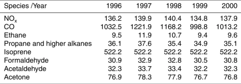
Table 1.Global annual total emissions for all species emitted in p-TOMCAT (in Tg yr−1).

Light-ning and aircraft NO_xemissions are not included here.

Species /Year 1996 1997 1998 1999 2000

NO_x 136.2 139.9 140.4 134.8 137.9

CO 1032.5 1221.9 1168.2 998.8 1013.2

Ethane 9.5 11.9 10.7 9.4 9.6

Propane and higher alkanes 36.1 37.6 35.4 34.9 35.1

Isoprene 522.2 522.2 522.2 522.2 522.2

Formaldehyde 30.9 32.9 32.8 30.5 30.8

Acetaldehyde 32.3 33.7 33.4 32.2 32.3

(24)

ACPD

9, 14023–14057, 2009

Title Page

Tables Figures

◭ ◮

Back Close

Full Screen / Esc

Table 2. Runs conducted for this study and how they differ. Interannually-varying fields are

denoted with “1996–2000” and fields without interannual variation are labelled “1996”. Note that “Clouds” are a subset of “Meteorology” in the current approach, meaning that in the case that meteorology is fixed to 1996 values (MetFix), clouds are kept fixed as well.

Emissions Meteorology Clouds

BASE 1996–2000 1996–2000 1996–2000

EmFix 1996 1996–2000 1996–2000

MetFix 1996–2000 1996 1996

CldFix 1996–2000 1996–2000 1996

(25)

ACPD

9, 14023–14057, 2009

Title Page

Tables Figures

◭ ◮

Back Close

Full Screen / Esc

Table 3.Global annual ozone budget terms for all the years of study (BASE run). The transport

term represents the STE for this global case.

1996 1997 1998 1999 2000

Net Chemistry (Tg/year) 658 581 380 466 662

Transport (Tg/year) 674 789 1012 859 627

(26)

ACPD

9, 14023–14057, 2009

Title Page

Tables Figures

◭ ◮

Back Close

Full Screen / Esc

Table 4. Regional annual ozone budget terms for the BASE run over Europe and Indonesia.

The transport term relates both to STE and to transport processes within the troposphere to and from the regions.

1996 1997 1998 1999 2000

EUROPE

Transport (Tg/year) −13 −15 −9 −8 −18

Deposition (Tg/year) −63 −63 −65 −65 −63

INDONESIA

Transport (Tg/year) −29 −32 −45 −32 −42

(27)

ACPD

9, 14023–14057, 2009

Full Screen / Esc

x

0.1 0.2 0.3 0.4 0.6 0.8 1.0 1.5

longitude [degrees] la ti tu d e [d e g r e e s ] longitude [degrees] la ti tu d e [d e g r e e s ]

Total Tropospheric NO2 column Standard Deviation (10

15_{molecules cm}-2₎

GOME p-TOMCAT

Mean Total Tropospheric NO2 column (10

15_{molecules cm}-2₎

0.0 0.3 0.6 1.0 2.0 3.0 4.0 6.0 8.0 10.

longitude [degrees] la ti tu d e [d e g r e e s ] GOME longitude [degrees] la ti tu d e [d e g r e e s ] p-TOMCAT a) b) c) d) 2 2

Fig. 1.Comparison of(a, b)annual 5-year mean p-TOMCAT tropospheric NO₂columns and(c,

d)their standard deviation, with GOME observations. The white area over North India denotes

total lack of observations during the 1996–2000 period. The purple (negative) areas relate to an artifact caused by the method used for the total column calculation (clean air subtraction –

see Savage et al. (2004) for further details). They appear only over remote areas where NO₂

(28)

ACPD

9, 14023–14057, 2009

Title Page

Tables Figures

◭ ◮

Back Close

Full Screen / Esc

Fig. 2.Percentage differences between tropospheric NO₂columns for each year and the 5-year

(29)

ACPD

9, 14023–14057, 2009

Title Page

Tables Figures

◭ ◮

Back Close

Full Screen / Esc

BASE - PAN column difference

1996

EmFix - PAN column difference

(%) longitude [degrees]

latitude

[d

egrees]

longitude [degrees]

lat

it

u

de

[degrees]

1997

1996

latitude

[d

egrees]

lat

it

ude

[deg

ree

s]

1997

-50. -30. -20. -10. -5.0 0.0 5.0 10. 20. 30. 50.

Fig. 3. 1996 and 1997 percentage differences of PAN tropospheric columns from the 5-year

mean for BASE and EmFix. The tropopause is the same as for Fig. 2.

(30)

ACPD

9, 14023–14057, 2009

Title Page

Tables Figures

◭ ◮

Back Close

Full Screen / Esc

lat

it

u

de

[deg

rees

]

BASE - Rn column difference 1996

lat

it

ude

[deg

rees

]

1999

-20. -10. -5.0 -2.0 -1.0 0.0 1.0 2.0 5.0 10. 20.

(%)

2

Fig. 4. 1996 and 1999 percentage di_fferences of radon tropospheric columns from the

5-year mean for three areas with high amplitude NO₂ deviations from the 5-year mean driven

(31)

ACPD

9, 14023–14057, 2009

Title Page

Tables Figures

◭ ◮

Back Close

Full Screen / Esc

Fig. 5. Percentage differences between tropospheric ozone columns for each year and the

(32)

ACPD

9, 14023–14057, 2009

Full Screen / Esc

Printer-friendly Version Interactive Discussion 1 2 -10 -8 -6 -4 -2 0 2 4 6 8 10

Globe

1996 1997 1998 1999 2000

Year O 3 B u rd e n d iff er enc e ( %)

11%

79%

6%

BASE EmFix MetFix CldFix P = 2 6 6 6 6 4 1 1 N N X i=0 X(i) S X(i) S 1 N N X i=0 X(i) B X(i) B 3 7 7 7 7 5 100 S

Fig. 6.Percentage global annual ozone burden differences from the 5-year mean as calculated

from the four sensitivity runs: BASE (blue), EmFix (red), MetFix (green) and CldFix (purple). The numbers at the upper right parts of the plots represent the amount of variability explained by each of the individual drivers: changing emissions (red), changing meteorology (green) and changing cloudiness (purple).

(33)

ACPD

9, 14023–14057, 2009

Title Page

Tables Figures

◭ ◮

Back Close

Full Screen / Esc

BASE

EmFix

MetFix

CldFix

1996 1997 1998 1999 2000

Year

O

3

B

u

rd

e

n d

iff

er

enc

e (

%)

Europe (9W,34E; 34N,66N)

-10 -8 -6 -4 -2 0 2 6 4 8

10 Indonesia (93E,136E; 16S,16N)

1996 1997 1998 1999 2000

Year

O

3

B

u

rd

e

n d

iff

er

enc

e (

%)

-20 -15 -10 -5 0 5 10 15 20

5% 86%

4%

32% 56% 6%

Fig. 7.Same as Fig. 6 but for the European and Indonesian boxes. Note the difference in the

(34)

ACPD

9, 14023–14057, 2009

Full Screen / Esc

Printer-friendly Version Interactive Discussion -6 -5 -4 -3 -2 -1 0 1 2 3 4 5 Ju l-9 6 O ct -9 6 Ja n -9 7 A p r-9 7 A u g -9 7 N o v -9 7 F e b -9 8 Ju n -9 8 S e p -9 8 D e c-9 8 M a r-9 9 Ju l-9 9 O ct -9 9 Ja n -0 0 M a y -0 0 A u g -0 0 Model Observa ons Sur fac e O 3 diff er e nc e (%) Year

Fig. 8. 12-month running means of ozone monthly differences from the 5-year (1996–2000)

mean for the Zugspitze research station (47◦N, 11◦E), as revealed by measurements (red) and

(35)