The persistence of common-ratio effects in multiple-play decisions
Michael L. DeKay
∗Dan R. Schley
∗Seth A. Miller
∗Breann M. Erford
∗Jonghun Sun
∗Michael N. Karim
∗Mandy B. Lanyon
†Abstract
People often make more rational choices between monetary prospects when their choices will be played out many times rather than just once. For example, previous research has shown that the certainty effect and the possibility effect (two common-ratio effects that violate expected utility theory) are eliminated in multiple-play decisions. This finding is challenged by seven new studies (N = 2391) and two small meta-analyses. Results indicate that, on average, certainty and possibility effects are reduced but not eliminated in multiple-play decisions. Moreover, in our within-participants studies, the certainty and possibility choice patterns almost always remained the modal or majority patterns. Our primary results were not reliably affected by prompts that encouraged a long-run perspective, by participants’ insight into long-run payoffs, or by participants’ numeracy. The persistence of common-ratio effects suggests that the oft-cited benefits of multiple plays for the rationality of decision makers’ choices may be smaller than previously realized.
Keywords: common-ratio effect, reverse common-ratio effect, certainty effect, possibility effect, multiple play, repeated play.
1
Introduction
In many instances, people make better, more rational deci-sions when they take a broad view of their situation rather than a narrow view (Kahneman & Lovallo, 1993; Read, Loewenstein & Rabin, 1999). For example, buying an ex-tended warranty for a particular electronic device may seem appealing when one is thinking only about that device, but thinking more broadly may make it easier to realize that the aggregate cost of such warranties over many appliances and devices almost certainly exceeds the expected cost of possi-ble failures. Assuming that such insurance is a moneymaker for the seller, insuring against relatively small losses that one can afford doesn’t make much sense, at least in terms of expected value (EV). Although this argument can be — and perhaps should be — applied to an individual purchase,
Dan R. Schley is now at Department of Marketing Management, Rotter-dam School of Management, Erasmus University, RotterRotter-dam, The Nether-lands. Jonghun Sun is now at Root Impact, Seoul, Korea. Michael N. Karim is now at Fors Marsh Group, LLC, Arlington, Virginia. Funding for Studies 1 and 2 was provided by National Science Foundation grant SES–0218318. We are grateful to Megan French, Rachael Martin, Elena Reynolds, and David Wanner for assistance conducting Studies 3–5 and to Hal Arkes, Tomás Lejarraga, Amanda Montoya, Ben Newell, and Dirk Wulff for their insightful comments on earlier versions of this manuscript. The first author wrote the initial version while a visiting researcher at the Center for Adaptive Rationality at the Max Planck Institute for Human De-velopment in Berlin, Germany.
Copyright: © 2016. The authors license this article under the terms of the Creative Commons Attribution 3.0 License.
∗Department of Psychology, The Ohio State University, 1835 Neil
Av-enue, Columbus, OH 43210. Email: [email protected].
†Department of Social and Decision Sciences, Carnegie Mellon
Univer-sity
many people find the notion of an expectation to be more compelling when they consider aggregating over numerous purchases.
Indeed, an ever-growing body of research has indicated that people are more likely to make decisions that are in ac-cord with EV theory or expected utility (EU) theory when they consider risky options whose outcomes will be aggre-gated over manyplays(for a review, see Wedell, 2011). For example, people are more likely to accept mixed gambles (those involving the possibility of a gain or a loss) with posi-tive EVs when they will be played multiple times rather than just once (Benartzi & Thaler, 1999; DeKay & Kim, 2005; Klos, 2013; Klos, Weber & Weber, 2005; Langer & Weber, 2001; Montgomery & Adelbratt, 1982; Redelmeier & Tver-sky, 1992; Wedell & Böckenholt, 1994). Similarly, for gam-bles involving either gains or losses (but not both), people are more likely to choose the higher-EV option in multiple play than in single play (Camilleri & Newell, 2013; Hais-ley, Mostafa & Loewenstein, 2008; Joag, Mowen & Gentry, 1990; Li, 2003; Su et al., 2013; but see Chen & Corter, 2006, for conflicting results). For gains, Wulff, Hills, and Hertwig (2015) recently extended this result to the situation in which participants learn about the probabilities and outcomes of the gambles via sampling (i.e., decisions from experience rather thandecisions from description; for reviews, see Her-twig, 2015; Hertwig & Erev, 2009). Additional studies have indicated that preference reversals (Wedell & Böckenholt, 1990), ambiguity aversion (Liu & Colman, 2009), and the description-experience gap (Camilleri & Newell, 2013) are also reduced in multiple play. Although most of these stud-ies have involved monetary gambles, the results appear to
extend to other situations as well (DeKay & Kim, 2005; Liu & Colman, 2009; Joag et al., 1990), at least when partic-ipants consider the aggregation of outcomes over multiple plays to be reasonable (DeKay & Kim, 2005; for related re-sults, see DeKay, 2011; DeKay, Hershey, Spranca, Ubel & Asch, 2006).1
1.1
Common-ratio effects
Previous research has also indicated thatcommon-ratio ef-fects are eliminated in multiple-play decisions (Barron & Erev, 2003, Study 5; Keren, 1991; Keren & Wagenaar, 1987). These effects, and their moderation in multiple play, are the focus of this article. Demonstrations of common-ratio effects require two choice problems: ascaled-up prob-lem and a scaled-downproblem. The possible outcomes in the two problems are identical, but the probabilities of the nonzero outcomes in the scaled-down problem are de-creased by the same factor relative to corresponding proba-bilities in the scaled-up problem. For example, in one ver-sion that we use, the scaled-up problem is a choice between Option A (a 100% chance of $60) and Option B (an 80% chance of $100, otherwise $0; hereafter, we omit the $0 outcome). In the scaled-down problem, the probabilities of winning in both options are divided by four (the common ra-tio) to yield a choice between A′(a 25% chance of $60) and B′ (a 20% chance of $100). The percentage of participants choosing the higher-EV option (B or B′, depending on the problem) is typically much higher in the scaled-down prob-lem than in the scaled-up probprob-lem; this discrepancy is the common-ratio effect. In this particular example, the discrep-ancy is also called acertainty effect(Kahneman & Tversky, 1979; Keren & Wagenaar, 1987), because one of the options in the scaled-up problem is a sure thing.
1We follow Camilleri and Newell (2013; and also Chen & Corter,
2006) in distinguishing betweenmultiple-playandrepeated-playsituations,
though we recognize that these terms have been used interchangeably in the past. In Camilleri and Newell’s usage, a typical, binary multiple-play sit-uation involves a single decision about a gamble (or a choice between two gambles) that will be played many times, with the same choice applying to all plays. A repeated-play situation, on the other hand, involves a string of identical single-play decisions in which the decision maker can make a different choice for each play. Although these two situations are clearly re-lated, they are empirically different (Camilleri & Newell, 2013), in part be-cause people do not naturally aggregate possible outcomes over a series of plays (Gneezy & Potters, 1997; Redelmeier & Tversky, 1992; Thaler, Tver-sky, Kahneman & Schwartz, 1997). Multiple-play and repeated-play deci-sions are normatively different as well, because the latter variety involves the option of changing one’s choice partway through the sequence. Aloy-sius (2007) noted that past disagreements regarding rationality in Samuel-son’s (1963) famous example (which involved a person declining one play but accepting 100 plays of a 50:50 gamble for $200 or –$100) can be at-tributed in part to Samuelson’s treating a multiple-play situation as if it were a repeated-play situation. Chen and Corter also noted this discrep-ancy. In the present article, we are primarily concerned with (a) descriptive rather than normative issues and (b) multiple-play rather than repeated-play decisions.
A common-ratio effect that involves very low probabili-ties in the scaled-down problem is called apossibility effect (Keren & Wagenaar, 1987). In our version, the scaled-up problem is a choice between C (a 90% chance of $50) and D (a 45% chance of $120) and the scaled-down problem is a choice between C′ (a 2% chance of $50) and D′ (a 1% chance of $120), where the chances of winning have been divided by 45. As before, the higher-EV option (D or D′) is typically much more popular in the scaled-down problem.
The modal choice pattern in these problems (e.g., choos-ing C in the scaled-up version and D′ in the scaled-down version of the possibility-effect example) violates EU the-ory. Under EU theory, choosing C over D implies that .90× u($50) > .45×u($120), which simplifies tou($50)/u($120) > 0.5. Similarly, choosing D′ over C′ implies that .02 × u($50) < .01×u($120), which simplifies tou($50)/u($120) < 0.5. These conclusions are contradictory; there is no utility function consistent with both preferences. By the same logic, the opposite patterns (choosing B and A′ in the certainty-effect example or D and C′in the possibility-effect example) also violate EU theory. These reverse patterns are less well known, but are common for some sets of problems (e.g., when the probabilities in the up and scaled-down problems differ by a smaller factor; Blavatskyy, 2010; Nebaut & Dubois, 2014).2
When discussing these issues, we find it useful to dis-tinguish between an effect and a choice pattern. For the problems considered in this article, we define the common-ratio effect (and the two special cases, the certaintyeffect and the possibilityeffect) as the empirical observation that participants are more likely to choose the riskier, higher-EV option in the scaled-down problem than in the correspond-ing scaled-up problem. This definition applies equally to between-participants and within-participants designs and is independent of theoretical explanations (e.g., regarding the relative weighting of certain and uncertain outcomes; Kah-neman & Tversky, 1979).3 Later in this article, we discuss
2That common-ratio and reverse common-ratio choice patterns violate
EU theory in single-play decisions does not necessarily imply that they do so in multiple-play decisions. To our knowledge, this question has not been addressed previously. Our initial analyses (see the Supplement) indicate that reverse common-ratio choice patterns can be consistent with EU theory in multiple play for some utility functions in the power family (Wakker, 2008). However, in our limited explorations of decision problems from Kahneman and Tversky (1979), Keren and Wagenaar (1987), Keren (1991), and Barron and Erev (2003, Study 5), we found no cases in which standard common-ratio choice patterns are consistent with EU theory in multiple play.
3This definition does not properly capture common-ratio effects in
prob-lems with equal-EV options (e.g., Kahneman & Tversky’s, 1979, Probprob-lems 7 and 8) or common-ratio effects in the domain of losses, where risk prefer-ences are often reversed (Kahneman & Tversky, 1979; Keren & Wagenaar, 1987, Study 1), but it is sufficient for our purposes. Also, we note that
Kahneman and Tversky did not use the termpossibility effect. Keren and
how the certainty effect, for example, reflects the relative frequencies of participants with the certaintychoice pattern (A and B′ in the above example) and participants with the reverse certaintychoice pattern(B and A′). Although these patterns are discernable only in within-participants designs in which participants respond to both the scaled-up and scaled-down problems, they are assumed to be present but unmeasured in between-participants designs (without this assumption, it would be impossible to infer utility violations from between-participants data).
In previous research, Keren and Wagenaar (1987, Study 1 and follow-up) showed that the certainty effect (or more precisely, a near-certainty effect, as they used a probabil-ity of .99 rather than 1.00 in their scaled-up problem) was eliminated when the gambles would be played ten times rather than just once. They obtained this result for both gains and losses in their Study 1. In their Study 2, Keren and Wagenaar showed that the possibility effect was elim-inated when the gambles would be played 100 times in-stead of once. Keren (1991) replicated Keren and Wage-naar’s results for the certainty effect using two different sets of problems and only five plays in the multiple-play condi-tion. In all of these studies, the common-ratio effects dis-appeared because the frequency of choosing the higher-EV option in the scaled-up problem increased in multiple play, whereas the frequency of choosing the higher-EV option in the scaled-down problem stayed about the same or increased only slightly. Li (2003) also reported that the frequency of choosing the higher-EV option in a scaled-up certainty-effect problem increased in multiple play, but that study did not include a corresponding scaled-down problem. Finally, Barron and Erev (2003, Study 5) reported that the certainty effect was eliminated and nearly reversed when very small gambles would be played 100 times.4 However, in contrast
to the other studies (and the effect of multiple plays more generally), this result was due primarily to a large decrease in the frequency of choosing the higher-EV option in the scaled-down problem. Taken together, these studies provide strong evidence that common-ratio effects are reduced or eliminated in multiple play, though Barron and Erev’s re-sults differ from the others in important ways. Table S.1 in the Supplement lists the gambles used in these studies.
1.2
Theoretical explanations
There is no generally accepted explanation for why people exhibit common-ratio effects in single-play choices. Expla-nations as varied as prospect theory (Kahneman & Tversky, 1979; Tversky & Kahneman, 1992), the transfer of
atten-follow Keren and Wagenaar’s usage.
4Barron and Erev’s (2003) article focused almost entirely on decisions
from experience rather than the more commonly studied decisions from de-scription (for more on the distinction, see Hertwig, 2015; Hertwig & Erev, 2009). However, their Study 5 involved only decisions from description.
tion exchange model (Birnbaum, 2008), the priority heuris-tic (Brandstätter, Gigerenzer & Hertwig, 2006), Mukher-jee’s (2010) dual-system model, decision field theory with distraction (Bhatia, 2014), and EU models with noise or se-quential sampling (Loomes, 2015) can account for at least some common-ratio effects. However, even theories that can explain common-ratio effects may fail to do so in specific instances. For example, Tversky and Kahneman’s (1992) best-fitting parameter values for cumulative prospect theory do not predict the possibility effect in Kahneman and Tver-sky’s (1979) original example.5 A more serious challenge
is that none of these theories tested thus far can explain the reverse common-ratio effects that occur for other pairs of problems (Blavatskyy, 2010; Nebaut & Dubois, 2014).
Regarding the general effects of multiple plays, Wedell (2011) noted that there are two basic types of explana-tions: those that assume a common process in single and multiple play and those that do not. In one example of a common-process explanation, Langer and Weber (2001) demonstrated that cumulative prospect theory can account for participants’ choices regarding mixed, positive-EV gam-bles in both single and multiple play when participants are shown (and the theory is applied to) the aggregate distri-bution of possible outcomes in the multiple-play condition. This result is consistent with the fact that participants are especially likely to accept multiple plays of (most) such gambles when presented with the full distribution of pos-sible outcomes (Benartzi & Thaler, 1999; DeKay, 2011; DeKay & Kim, 2005; Klos, 2013; Langer & Weber, 2001; Redelmeier & Tversky, 1992; for an exception, see Keren, 1991). The generality of common-process explanations is limited, however, by the difficulty of envisioning or calcu-lating the relevant features of outcome distributions when they are not provided (Benartzi & Thaler, 1999; Klos, 2013; Klos et al., 2005). This problem may be especially acute for common-ratio effects because most of the choices involve two risky options rather than one.
In our view, a more likely explanation for the effects of multiple plays is that the decision processes are more thor-ough and integrative in multiple play than in single play (Wedell, 2011). For example, participants find EV informa-tion to be more relevant (Montgomery & Adelbratt, 1982) and report using more complex strategies (Wedell & Böck-enholt, 1994) in multiple-play decisions. Evidence from functional measurement (Joag et al., 1990) and eye
track-5In Kahneman and Tversky’s (1979) Problem 7 (the scaled-up
ing (Su et al., 2013) also indicates that participants are more likely to use multiplicative or weighting-and-adding processes in multiple play than in single play. Most re-cently, Wulff et al. (2015) reported that in a decisions-from-experience task involving pairs of gambles, partici-pants who anticipated making a multiple-play choice rather than a single-play choice tried out the gambles more times before deciding which one to play. Perhaps ironically, these studies suggest that people are more likely to use compli-cated decision strategies in multiple play, where such strate-gies are more difficult to apply.
1.3
Seven new studies
In what follows, we report seven new studies regarding the possible reduction or elimination of common-ratio effects in multiple-play decisions. Our goal was not to resolve the process issues raised above, though some of our data do bear on the question of whether proper aggregation of long-run payoffs is sufficient to eliminate common-ratio effects. Nor was our goal to replicate or not replicate other researchers’ results, though that is how the project evolved. Instead, our original intent was to assess whether the elimination of common-ratio effects in multiple-play decisions — a finding that we considered relatively well established — would be moderated by participants’ views regarding the reasonable-ness of aggregating outcomes over multiple plays (i.e., the perceived fungibilityof the outcomes; DeKay & Kim, 2005; see the Supplement for details regarding our rationale). Al-though we predicted that multiple plays would diminish the certainty and possibility effects when outcome aggre-gation is reasonable, both effects remained large and sig-nificant in multiple-play decisions involving monetary gam-bles for oneself. Surprised by these initial results, we con-ducted several additional studies in which we attempted to strengthen the multiple-play manipulation by (a) increasing the number of plays, (b) improving the clarity and salience of the relevant wording, (c) creating additional conditions that were intended to encourage participants to think about aggregate outcomes in multiple play, and (d) playing par-ticipants’ choices for real money (in one study). Despite these and other efforts (e.g., using both within- and between-participants designs), certainty and possibility effects almost always remained significant in multiple-play decisions.
For ease of exposition, we present our seven studies to-gether rather than separately. We first describe our gen-eral experimental approach, noting the most important dif-ferences among our studies, and then use simple graphs to compare our results to those of earlier authors. After illus-trating our basic statistical model using data from a few ex-ample studies, we present two small meta-analyses (separate analyses for certainty and possibility effects) that integrate the results of our new studies with those from previous re-search. We then look in greater detail at the choice patterns
in our within-participants studies. Finally, we examine the additional conditions that were designed to encourage par-ticipants to think about aggregate outcomes and we assess whether the effects of multiple plays are moderated by two individual differences. Considering the old and new stud-ies together, the overall results indicate that common-ratio effects are much more persistent in multiple play than pre-viously thought.
2
Method
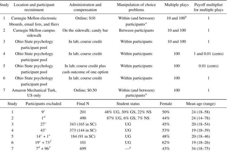
Table 1 provides an overview of study characteristics, sam-ple sizes, and participant demographics in our seven studies.
2.1
General procedures
In each study, we randomly assigned participants to the 1-play, 10-1-play, and 100-play conditions. The first part of Study 1 omitted the 100-play condition, whereas Studies 4– 7 omitted the 10-play condition (i.e., we increased the num-ber of plays in the later studies). In our standard design, par-ticipants in each condition made 11 choices between options like those described in Table 2, with each problem shown on a separate screen of the computer-based survey. For exam-ple, Problem 10 was presented as follows in the single-play [multiple-play] condition:
Option A:
45% chance [on each gamble] that you get $120 55% chance [on each gamble] that you get no money Option B:
90% chance [on each gamble] that you get $50 10% chance [on each gamble] that you get no money6
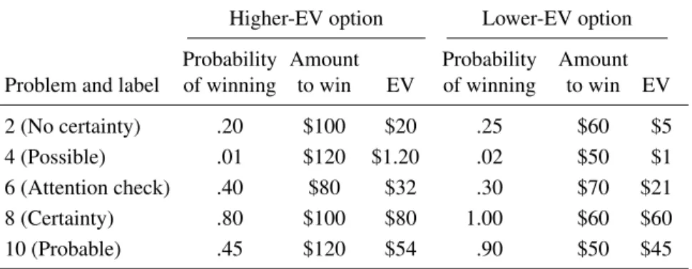
Problems 2 and 8 (based on Keren, 1991) provided a within-participants test of the certainty effect (as in Kah-neman & Tversky, 1979, and Barron & Erev, 2003) and Problems 4 and 10 (based on Keren & Wagenaar, 1987) provided a within-participants test of the possibility effect (as in Kahneman & Tversky, 1979). Treating problem as a within-participants variable allowed us to assess partici-pants’ choice patterns, as noted above (in contrast, the num-ber of plays was always a between-participants variable). Problem 6 provided an attention check in which one op-tion dominated the other. Participants who did not chose the dominant option in Problem 6 or who did not make all four of the key choices (Problems 2, 4, 8, and 10) were excluded
6In the multiple-play version of Problem 2 (the scaled-down,
Table 1: Study characteristics, sample sizes, and participant demographics
Study Location and participant recruitment
Administration and compensation
Manipulation of choice problems
Multiple plays Payoff multiplier for multiple plays 1 Carnegie Mellon electronic Online; $10 Within (and between) 10 and 100b 1
bboards, email lists, and fliers participantsa
2 Carnegie Mellon campus sidewalk
On the sidewalk; candy bar Between participants 10 and 100 1
3 Ohio State psychology In lab; course credit Within participants 10 and 100 1 participant pool
4 Ohio State psychology In lab; course credit Within participants 100 1 and 0.01 (cents) participant pool
5 Ohio State psychology In lab; course credit plus Within participants 100 0.01 (cents) participant pool cash outcome of one option
6 Ohio State psychology In lab; course credit Within participants 100 1 participant pool
7 Amazon Mechanical Turk, US only
Online; $0.50 Within (and between) participantsa
100 1
Study Participants excluded Final N Student status Female Mean age (range)
1 9c 201 48% UG, 30% GS, 22% NS 50% 24 (18–58)
2 1d 490 87% UG, 6% GS, 7% NS 44% 24 (14–78)
3 27c 343 (165 in SC) UG 45% 20 (18–54)
4 43c 373 (144 in SC) UG 53% 19 (18–39)
5 14c+ 1e 184 (91 in SC) UG 48% 20 (18–46)
6 19c+ 73f 101 UG 62% 19 (18–26)
7 7d+ 96f 699 —g 43% 34 (18–75)
Note. UG = undergraduates. GS = graduate students. NS = nonstudents. SC = standard conditions, with no additional questions or statements designed to encourage the long-run perspective.
aBecause problem order was reversed for half of the participants, the first half of the data can be treated as a between-participants study. b
Study 1 had two parts: Study 1a involved 1 or 10 plays, whereas Study 1b involved 1, 10, or 100 plays. Otherwise, the questions were identical. See the Supplement for details.
cExcluded for failing the attention check and/or not answering a key choice question. d
Excluded for not answering a key choice question (there was no attention check). eExcluded for suspecting that cash payments would not be made (they were). f Excluded for failing the manipulation check.
g
Not assessed.
from all analyses. The six odd-numbered problems were in-cluded to reduce the likelihood that participants would no-tice the relationships between the problems of interest; these filler problems are not discussed further. In 5 of the 11 prob-lems, the option presented first had the higher EV. Payoffs were hypothetical in all studies except Study 5 (see below). In the multiple-play conditions, participants were told that each of the two options “involves a series often[one hundred] monetary gambles.” After the options were de-scribed, but before participants made their choice, they were told, “Your choice between options A and B applies to all
ten[one hundred] gambles.” Before the very first choice,
participants were also told, “You may not choose option A for some gambles and option B for others.” In Experiments 4–7, they were also told, “Regardless of your choice, the outcome of any particular gamble in the sequence (say the 23rd gamble) has no effect on the outcome of any other ble in the sequence (say the 24th gamble or the 67th gam-ble). Each gamble is independent of the others.” Study 7 included an additional analogy to “flipping a coin or rolling a die over and over again.”
Table 2: Critical problems, gambles, and expected values (EVs) in the single-play condition
Higher-EV option Lower-EV option
Probability Amount Probability Amount
Problem and label of winning to win EV of winning to win EV
2 (No certainty) .20 $100 $20 .25 $60 $5
4 (Possible) .01 $120 $1.20 .02 $50 $1
6 (Attention check) .40 $80 $32 .30 $70 $21
8 (Certainty) .80 $100 $80 1.00 $60 $60
10 (Probable) .45 $120 $54 .90 $50 $45
Note. All options except the certain option in Problem 8 included a complemen-tary outcome of “no money”. Labels and EVs were not shown to participants. The six odd-numbered problems were fillers and are omitted here. Studies 2 and 7 used only Problems 2, 4, 8, and 10. Gambles in Studies 4–6 had lower stakes (one tenth as large for these critical problems). Table S.2 in the Supplement lists all problems used in the single-play condition of Studies 1–7.
stressed that the gamble would be played ONE,TEN, or
ONE HUNDRED times. In this article, we focus almost
exclusively on the binary choices, for consistency with pre-vious research. In Study 7, we included the words ONE AND ONLY ONE play and ONE HUNDRED plays in the response options as well as the questions. In every study, participants answered a few debriefing questions and pro-vided demographic information at the end of the survey.
2.2
Primary differences among studies
Study 1 had two parts. Study 1a was designed to assess the role of perceived fungibility in multiple-play decisions. In this article, we consider only those conditions involving monetary gambles for oneself (there were several other con-ditions; see the Supplement) and ignore all questions related to fungibility. In Study 1b, we simplified the design by us-ing only monetary gambles for oneself, but added a 100-play condition to strengthen the multiple-play manipulation. The results of Studies 1a and 1b are combined for analysis.
The most obvious difference between our Study 1 and Keren and Wagenaar’s (1987) studies is that we assessed the certainty and possibility effects within participants (as did Barron & Erev, 2003, for the certainty effect) rather than between participants. In Study 2, we adopted a completely between-participants design similar to that in Keren and Wa-genaar’s studies, with each participant making only one of the four key choices (Problem 2, 4, 8, or 10) in either the 1-play, 10-play, or 100-play condition. In order to collect a large sample relatively quickly, we administered the study as a short paper-based survey on a busy university sidewalk. After Study 2, we returned to our within-participants
ap-proach. In addition to the standard conditions (described above), Studies 3–5 also included one or more conditions designed to encourage participants to adopt a long-run per-spective. These conditions might be expected to facilitate the choice of the higher-EV option, thereby reducing the certainty and possibility effects, especially in multiple play. Additionally, because reasoning about gambles (and mul-tiple plays of gambles) requires a degree of mathematical ability or intuition, we hypothesized that the effects of mul-tiple plays might be more pronounced for participants who are better at math. In Studies 4–6, we examined the possi-ble moderating effects of participants’numeracy, defined as “the ability to process basic probability and numerical con-cepts” (Peters, Västfjäll, Slovic, Merz, Mazzocco & Dick-ert, 2006, p. 407; also see Peters, 2012), using an estab-lished eight-item scale (Weller, Dieckmann, Tusler, Mertz & Peters, 2013). We discuss these additional conditions and measures later, after our main results.
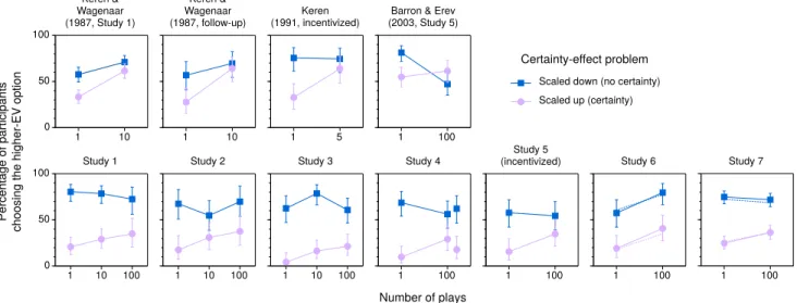
Figure 1: Percentages of participants choosing the higher-EV option in problems related to the certainty effect in previous studies (top) and in the standard conditions of our studies (bottom). In Study 4, the results for 100 plays with cents appear to the right of those for 100 plays with dollars. In Studies 6 and 7, solid lines show results for participants who answered the manipulation-check question correctly; dotted lines (without error bars) show results for all participants. Error bars indicate 95% CIs.
1 10 100 0
50 100
1 10 1 5 1 100
1 10 100 1 10 100 1 100 1 100
Number of plays
Percentage of participan
ts
choosing the highe
r-EV option
Keren & Wagenaar (1987, Study 1)
Keren & Wagenaar (1987, follow-up)
Keren (1991, incentivized)
Barron & Erev (2003, Study 5)
Study 1 Study 2 Study 3 Study 4
Study 5 (incentivized)
Certainty-effect problem
1 100
Study 6 Study 7
1 100
1 10
0 50 100
Scaled down (no certainty)
Scaled up (certainty)
played either one time (for dollars) or 100 times (for cents), depending on each participant’s condition.7
Although participants were reminded of the number of plays many times (e.g., the numberONE HUNDRED ap-peared 34 times in the standard multiple-play condition of Studies 4 and 5), the results made us wonder whether some participants had simply tuned out that information. Studies 6 and 7 included manipulation checks that asked participants how many times their chosen option would be played in each choice (Study 6) or in the choice they just made (Study 7). Our primary analyses are restricted to participants who answered correctly (including all participants yielded very similar results). Study 7 was our largest study, conducted on Amazon Mechanical Turk. It differed from the other studies in that participants answered either the two certainty-effect problems or the two possibility-certainty-effect problems, with-out any fillers. We had initially envisioned Study 7 as a much stronger version of our between-participants Study 2, but decided that there was no harm in adding a second prob-lem. Because we manipulated problem order, the first half of the data could still be treated as a between-participants study (this was also true of Study 1, in which the order of the 11 problems was reversed for half of the participants). For additional details and the surveys themselves, see the Supplement.
7Keren (1991) used a somewhat similar procedure, though payoffs in
the multiple-play (5-play) condition were not reduced and only one partic-ipant from each group of 8 to 12 was paid.
3
Results
3.1
Visual comparisons between studies
Figure 1 presents results for the certainty effect, with pre-vious studies in the top row and the standard conditions of our studies in the bottom row. In each panel, a certainty effect occurred whenever the higher-EV option was signifi-cantly more likely to be chosen in the scaled-down problem, which did not include a certain option, than in the scaled-up problem, which did.
A few basic results are evident in the figure. First, cer-tainty effects were obtained in the single-play conditions of all of the studies, though they were generally larger in our studies than in previous studies. Second, in the multiple-play conditions, certainty effects remained relatively large in most of our studies, whereas they essentially disappeared in Keren and Wagenaar’s (1987) and Keren’s (1991) stud-ies and were reversed in Barron and Erev’s (2003) study (note the large drop for the scaled-down problem in Barron and Erev’s data). Certainty effects were somewhat smaller in multiple play than in single play in most of our studies as well, though the larger spread in our studies makes the magnitudes of these reductions difficult to assess visually. Finally, it appears that there was not a reliable difference between the results for 10 and 100 plays in our studies.
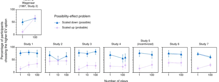
possibil-Figure 2: Percentages of participants choosing the higher-EV option in problems related to the possibility effect in a previous study (top) and in the standard conditions of our studies (bottom). In Study 4, the results for 100 plays with cents appear to the right of those for 100 plays with dollars. In Studies 6 and 7, solid lines show results for participants who answered the manipulation-check question correctly; dotted lines (without error bars) show results for all participants. Error bars indicate 95% CIs.
1 10 100 0
50 100
1 100
0 50 100
Scaled down (possible)
Scaled up (probable)
1 10 100 1 10 100 1 100 1 100
Percentage of participan
ts
choosing the highe
r-EV option
Number of plays
Keren & Wagenaar (1987, Study 2)
Study 1 Study 2 Study 3 Study 4
Study 5 (incentivized)
Possibility-effect problem
1 100
Study 6 Study 7
1 100
ity effects were large in both the single- and multiple-play conditions, in contrast to the disappearance of the effect in the multiple-play condition of Keren and Wagenaar’s (1987) study. Possibility effects were smaller in our between-participants Study 2 than in our other studies, but the results did not match those of Keren and Wagenaar’s study either. As was the case for certainty effects, there was no consistent difference between the results for 10 and 100 plays in our studies. Overall, certainty and possibility effects appeared more persistent in our studies than in previous studies.
In Studies 1–6, participants made a preference rating be-fore choosing an option in each problem. Graphical re-sults for mean preference ratings (see Figure S.1 in the Supplement) were nearly identical to those for choice pro-portions. Moreover, the choice-proportion results for Study 7, in which choices were not preceded by preference rat-ings, were very similar to those for Studies 1–6 (see Figures 1 and 2), suggesting that the preference ratings had little if any effect on participants’ subsequent choices. We do not consider the preference ratings further.
Because we manipulated problem order in Studies 1 and 7, considering only the first half of the data yielded a between-participants study in each case. Figure 3 indicates that the results for the first half of the data look similar to those for the full studies (see the corresponding panels in Figures 1 and 2). The one exception was that, in Study 7, the effect of multiple plays on the possibility effect was notably stronger when only the first half of the data was considered. However, in contrast to Keren and Wagenaar’s (1987, Study 2) results for the possibility effect (see Figure 2), about half
of the reduction in Study 7 was due to a decrease in the per-centage of participants choosing the higher-EV option in the scaled-down problem in multiple play (see Figure 3).
Figure 3: Percentages of participants choosing the higher-EV option in problems related to the certainty effect (top) and the possibility effect (bottom) in the first half of our Studies 1 and 7 (between-participants comparisons). Error bars indicate 95% CIs.
1 100 Study 7
1 100 1 10 100
0 50 100
Scaled down (no certainty)
Scaled up (certainty)
1 10 100 0
50 100
Scaled down (possible)
Scaled up (probable) Certainty-effect problem
Possibility-effect problem
Number of plays
Percentage of participan
ts
choosing the highe
r-EV option
Study 1
3.2
Illustrative analyses
For each effect (certainty or possibility) in each study, we used logistic regression to predict the choice of the higher-EV option on the basis of problem (scaled-up problem = –1/2, scaled-down problem = +1/2), plays (single play = –1/2, multiple play = +1/2), and their interaction. The vari-ables were coded so that a positive effect of problem would indicate the expected certainty or possibility effect and a positive coefficient for plays would indicate a greater like-lihood of choosing the higher-EV option in multiple play. A reduction in the magnitude of a certainty or possibility effect in multiple play would be evidenced by a negative co-efficient for the interaction. For brevity, we present detailed results for only a few illustrative studies.
For Keren and Wagenaar’s (1987, Study 1) certainty-effect data (see Figure 1), there was a significant positive effect of problem,b= 0.71, 95% CI [0.39, 1.04],OR= 2.04, χ2(1) = 18.61,p< .001; a significant positive effect of plays, b= 0.88, CI [0.55, 1.20],OR= 2.40,χ2(1) = 28.38,p< .001; and a nearly significant negative interaction,b= –0.57, CI [–1.23, 0.08], OR= 0.56, χ2(1) = 2.93, p = .087. These statistics essentially recreate Keren and Wagenaar’s results, but with the addition of coefficients and confidence inter-vals. For Keren and Wagenaar’s (1987, Study 2) possibility-effect data (see Figure 2), all three possibility-effects were significant: b = 0.99, CI [0.45, 1.53], OR= 2.69, χ2(1) = 13.71, p < .001 for problem; b = 1.69, CI [1.15, 2.23], OR = 5.41, χ2(1) = 42.69,p< .001 for plays; andb= –2.14, CI [–3.22, –1.06],OR= 0.12,χ2(1) = 16.02,p< .001 for the interac-tion. For both the certainty and possibility effects, the Prob-lem×Plays interaction was attributable to the increased ap-peal of the higher-EV option in the scaled-up problem in multiple play.
In our Study 1, which had rather typical results for our studies, we used repeated-measures logistic regressions be-cause each participant responded to both the scaled-up and scaled-down problems.8 For ease of comparison across
studies, we ignored the distinction between the 10- and 100-play conditions in our primary models. For the certainty effect (see Figure 1), there was a significant positive effect of problem,b= 2.37, CI [1.85, 2.88],OR= 10.66,χ2(1) = 75.04,p< .001, but the effect of plays,b= 0.15, CI [–0.29, 0.60],OR= 1.17,χ2(1) = 0.46,p= .50, and the interaction, b= –0.78, CI [–1.81, 0.24], OR= 0.46, χ2(1) = 2.29,p= .13, were not significant. For the possibility effect in Study 1 (see Figure 2), there were significant positive effects of problem, b = 2.58, CI [2.02, 3.14], OR = 13.23, χ2(1) = 79.68, p < .001, and plays,b = 0.56, CI [0.12, 0.99], OR = 1.75,χ2(1) = 6.07,p= .013, but the interaction was not significant,b= –0.90, CI [–2.01, 0.21],OR= 0.41,χ2(1) = 2.60,p= .11.9 In contrast to Keren and Wagenaar’s (1987)
8We used SAS PROC GENMOD regardless of whether problem was
varied between or within participants. When there was more than one ob-servation per participant, GENMOD used generalized estimating equations that yielded population-average estimates. Conceptually, these estimates are more comparable to those from completely between-participants stud-ies than are the average unit-specific (participant-specific) estimates from random-effects models. Although population-average and unit-specific es-timates typically differ for nonlinear models (Hu, Goldberg, Hedeker, Flay & Pentz, 1998; Raudenbush & Bryk, 2002, pp. 303–304), random-effects models fit using SAS PROC GLIMMIX yielded identical or nearly identi-cal results in our studies.
9Results were similar when we used orthogonal contrast codes to
results, the certainty and possibility effects remained signifi-cant in multiple play (see below). In summary, the results of our Study 1 did not replicate those of Keren and Wagenaar (1987) especially well, though the signs of the coefficients were the same in all of the above regressions.
3.3
Two small meta-analyses
In order to resolve apparently conflicting results like those above, we conducted two small meta-analyses: one for the certainty effect (11 studies) and one for the possibility ef-fect (8 studies).10 For simplicity, we considered only the
standard conditions from our studies; conditions designed to promote a long-run view are discussed later. In addition, we considered all multiple-play conditions to be the same, regardless of the number of plays (see footnote 9), and col-lapsed across multiple-play conditions involving dollars and cents in Study 4.
These analyses also compared effects from studies in which certainty and possibility effects were assessed within participants (most of our studies plus Barron & Erev’s, 2003, Study 5) or between participants (our Study 2 plus Keren & Wagenaar’s, 1987, studies and Keren’s, 1991, study).11 This approach is appropriate because the effect
sizes are in a common metric (a logistic regression coeffi-cient, which is the natural log of an odds ratio) and the stan-dard errors of the effect sizes correctly reflect the sample sizes and experimental designs.12 An additional criterion is
or possibility effects), allps≥.40. Similar results were obtained for the
second code in Studies 2 and 3 (the only other studies with both 10- and
100-play conditions), allps≥.072. Of the six possible interactions
involv-ing the second code in Studies 1–3, only three had the anticipated negative sign (see Figures 1 and 2). Thus, the distinction between 10 and 100 plays did not have a reliable effect on certainty and possibility effects in our stud-ies.
10Greg Barron (personal communication, 2003) provided the data for
Barron and Erev’s (2003) Study 5 (see Table S.3 in the Supplement).
11Keren’s (1991) experimental design involved two parallel (i.e.,
sim-ilar, but not identical) sets of gambles. For single play (n= 49), some
participants received the certainty problem (like our Problem 8) from one set and the no-certainty problem (like our Problem 2) from the other set, whereas others received the reverse. A similar procedure was used for
mul-tiple play (n= 47). Because different participants received the certainty
and no-certainty problems in each set, Keren treated problem as a between-participants variable. We also analyzed Keren’s study in this way. How-ever, because Keren collapsed across the two parallel sets of gambles, each participant contributed two choices, doubling the sample size for the rele-vant statistical tests (e.g., the number of observations in Keren’s Table 1 is
192, twice the trueNof 96). To address this sample-size issue (but not the
related independence issue), we divided the counts in Keren’s Table 1 by two. Because doing so yielded some noninteger counts, we conducted our analysis twice, once with counts rounded up and once with counts rounded down, and then averaged the results. This procedure increased the standard
errors of the logistic regression coefficients (relative to those forN= 192),
but otherwise had no effect on our substantive results. Though imperfect, this solution is preferable to omitting the study from our meta-analysis.
12Rescaling the effect sizes to express them in a common metric, as
sug-gested by Morris and DeShon (2002) forstandardizedeffect sizes
aris-ing from within- and between-participants studies, is not necessary in our
case because we useunstandardizedregression coefficients from otherwise
that the effect sizes from the two designs estimate the same treatment effect (Morris & DeShon, 2002). This require-ment is plausibly satisfied in our case (see footnote 8), but the effect sizes may differ among studies nonetheless (e.g., because of different instructions and monetary amounts). We addressed these differences by treating study as a ran-dom effect, to allow for unexplained variability.13
For both the certainty effect and the possibility effect, we present results for three different (but not independent) ef-fect sizes: (a) the simple efef-fect of problem in the single-play condition, which gives the magnitudes of the classic cer-tainty and possibility effects, (b) the simple effect of prob-lem in the multiple-play condition, and (c) the difference between the these two, which gives the reductions in the certainty and possibility effects in multiple play. The third effect size is equal to the logistic regression coefficient for the Problem ×Plays interaction, but here we reverse the sign so that a positive value denotes a reduction.14
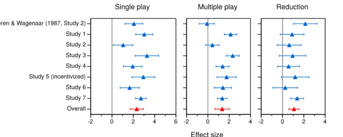
Results for the certainty effect appear in Figure 4. The left panel shows that the certainty effect in single play was somewhat larger in our studies than in previous studies. Across all studies, the overall effect size wasb= 1.98, CI [1.47, 2.50], OR= 7.26, t(10) = 8.61, p < .001, meaning that the odds of choosing the higher-EV option were sub-stantially greater when the choice was between two uncer-tain options (as in Problem 2) than when one of the options was certain (as in Problem 8). The results for multiple play, shown in the center panel, are more striking. In all four of the earlier studies, the certainty effect was eliminated in multiple play, with Barron and Erev’s (2003) data showing a nearly significant reversal. In contrast, six of our seven stud-ies yielded a significant residual certainty effect. The overall effect in multiple play remained sizeable and significant,b = 1.08, CI [0.49, 1.67],OR= 2.95,t(10) = 4.08,p = .002. The right panel indicates the reduction in the certainty ef-fect in multiple play relative to single play. Despite the fact that only 3 of the 11 studies found significant reductions, the overall reduction was substantial and significant,b= 0.97, CI [0.58, 1.36],OR= 2.64,t(10) = 5.51,p< .001. The re-duction was similar when our Studies 1 and 7 were treated as between-participants studies (i.e., when only the first half of the data was considered),b= 0.88, CI [0.41, 1.36],OR= 2.41,t(10) = 4.13,p= .002, and when only our seven studies
identical models.
13In random-effects meta-analysis, the overall effect size is an estimate
of the mean of a distribution of population effect sizes rather than an es-timate of a single population effect size (Shadish & Haddock, 2009). The random-effects model reduces to the fixed-effect model when the between-study variance is estimated to be zero. We report results from random-effects meta-analyses, but fixed-effect meta-analyses yielded similar con-clusions.
14For each study, the third effect size is equal to the difference between
Figure 4: Meta-analysis results for the certainty effect in single- and multiple-play decisions. Error bars indicate 95% CIs.
-2 0 2 4 -2 0 2 4
Overall Study 7 Study 6 Study 5 (incentivized) Study 4 Study 3 Study 2 Study 1 Barron & Erev (2003, Study 5) Keren (1991, incentivized) Keren & Wagenaar (1987, follow-up) Keren & Wagenaar (1987, Study 1)
-2 0 2 4 6
Reduction Multiple play
Single play
Effect size
(logistic regression coefficient = ln(odds ratio))
Figure 5: Meta-analysis results for the possibility effect in single- and multiple-play decisions. Error bars indicate 95% CIs.
-2 0 2 4
-2 0 2 4
Effect size
(logistic regression coefficient = ln(odds ratio)) Reduction Multiple play
Overall Study 7 Study 6 Study 5 (incentivized) Study 4 Study 3 Study 2 Study 1 Keren & Wagenaar (1987, Study 2)
-2 0 2 4 6
Single play
were considered,b= 0.85, CI [0.36, 1.34],OR= 2.34,t(6) = 4.25,p= .005.
Results for the possibility effect appear in Figure 5. In single play (left panel), all eight studies yielded signifi-cant effects, though the effect was barely signifisignifi-cant in our between-participants Study 2. The overall effect wasb = 2.33, CI [1.71, 2.95],OR= 10.29,t(7) = 8.88,p< .001. In multiple play (center panel), the possibility effect was com-pletely absent in Keren and Wagenaar’s (1987) study, but remained significant in six of our seven studies. The overall effect wasb= 1.34, CI [0.65, 2.02],OR= 3.81,t(7) = 4.62,p = .002. Although the reduction in the possibility effect in the multiple-play condition (right panel) was significant in only two of the eight studies, the overall reduction was substan-tial and significant,b= 1.07, CI [0.58, 1.54],OR= 2.91,t(7) = 5.19,p= .001. Again, the reduction was similar when our Studies 1 and 7 were treated as between-participants stud-ies, b= 1.10, CI [0.42, 1.78], OR= 2.83, t(7) = 3.84,p=
.006, and when only our studies were considered,b= 0.95, CI [0.46, 1.44],OR= 2.58,t(6) = 4.77,p= .003.
3.4
Unpacking the within-participants results
op-Figure 6: Percentages of participants with each of the possible choice patterns in problems related to the certainty and possibility effects in the standard conditions of our six within-participants studies. Error bars indicate 95% CIs, but these ignore between-study variability.
Both lower-EV
options
Possibility pattern
Reverse possibility pattern
Both higher-EV
options
Percentage of participan
ts
with each choice pattern
Certainty effect Possibility effect
Both lower-EV
options
Certainty pattern
Reverse certainty pattern
Both higher-EV
options 0
20 40 60 80
Single play
Multiple play
tions (HH%), choosing the higher-EV option in Problem 2 and the lower-EV option in Problem 8 (the certainty pat-tern, C%), and choosing the lower-EV option in Problem 2 and the higher-EV option in Problem 8 (the reverse certainty pattern, RC%). The fourth pattern, choosing both lower-EV options, is not directly relevant. The percentage of partici-pants choosing the higher-EV option in Problem 2 is HH% + C% and the percentage choosing the higher-EV option in Problem 8 is HH% + RC%. The difference between these two percentages (the basis for our measure of the certainty effect in the preceding analyses) is thus C% – RC%. For this difference-based measure, a certainty effect is observed whenever there is a systematic imbalance between the two choice patterns. More important, any decrease in this mea-sure in multiple play could be due to a decrease in C%, an increase in RC%, or a combination of changes (e.g., a larger decrease for C% than for RC%). Analogous logic applies to the possibility effect.
Within-participants designs are appealing in this context precisely because they provide this level of detail. Figure 6 shows the percentages of participants with each of the four possible choice patterns for problems related to the certainty effect (Problems 2 and 8) and, separately, for problems re-lated to the possibility effect (Problems 4 and 10) in the stan-dard conditions of our six within-participants studies. For simplicity, we have aggregated across the 10- and 100-play conditions in Studies 1 and 3, across the dollars and cents conditions in Study 4, and across studies (ns = 1027 and 1076 for the certainty and possibility effects, respectively). (Tables S.4–S.14 in the Supplement provide counts and per-centages for all choice patterns separately for all conditions of all of our studies.)
The percentage of participants exhibiting the certainty choice pattern in Problems 2 and 8 dropped from 56.3%
in single play to 48.1% in multiple play. Random-effects meta-analyses revealed that this reduction was significant for our data, overallb = 0.39, CI [0.06, 0.72],OR= 1.47, t(5) = 3.00, p= .030, and when Barron and Erev’s (2003) data were also included (totaln= 1188), overallb= 0.49, CI [0.16, 0.82],OR= 1.63,t(6) = 3.61,p= .011 (for Bar-ron & Erev’s data alone, the drop from 33% in single play to 10% in multiple play was significant,OR= 4.42, Fisher exactp< .001).15 In contrast to Barron and Erev’s results,
the certainty pattern remained the modal choice pattern in multiple-play decisions in five of our six within-participants studies and was the majority pattern in Studies 1 and 3 (in Study 5, the modal pattern in multiple play was choosing the lower-EV option in both problems). In Problems 4 and 10, the percentage of participants exhibiting the possibility choice pattern dropped from 61.1% to 47.0% in our studies, overallb = 0.63, CI [0.29, 0.97], OR= 1.88, t(5) = 4.76, p = .005. The possibility pattern remained the modal pat-tern in multiple-play decisions in all six studies and was the majority pattern in Studies 1, 3, and 5.
The prevalence of the reverse certainty pattern increased from 4.6% in single play to 8.4% in multiple play (see the left panel of Figure 6). This increase was nearly significant in our data, overallb= 0.66, CI [–0.18, 1.50], OR= 1.93, t(5) = 2.02,p= .099, and was significant when Barron and Erev’s (2003) data were also included, overallb= 0.80, CI [0.04, 1.57], OR= 2.24,t(6) = 2.58,p = .042 (for Barron & Erev’s data alone, the increase was from 7% to 24%,OR = 4.54, Fisher exact p =.003). For the reverse possibility pattern, the increase from 4.0% to 7.1% in our data was not
15For consistency with our other meta-analyses, these reductions are
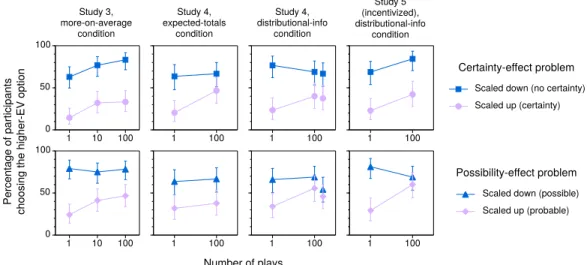
Figure 7: Percentages of participants choosing the higher-EV option in problems related to the certainty effect (top) and the possibility effect (bottom) in the long-run-prompt conditions of our Studies 3–5. In the distributional-info condition of Study 4, the results for 100 plays with cents appear to the right of those for 100 plays with dollars. Error bars indicate 95% CIs.
1 10 100 0
50 100
1 10 100 0
50 100
Certainty-effect problem
Possibility-effect problem
Study 3, more-on-average
condition
Number of plays
Percentage of participan
ts
choosing the
higher-EV option 1 100
Scaled down (no certainty)
Scaled up (certainty)
1 100
1 100
Scaled down (possible)
Scaled up (probable)
1 100
1 100
1 100
Study 5 (incentivized), distributional-info
condition Study 4,
distributional-info condition Study 4,
expected-totals condition
significant, overallb = 0.47, CI [–0.42, 1.36],OR= 1.60, t(5) = 1.36,p= .23 (see the right panel of Figure 6).
Overall, the moderating effects of multiple plays were less impressive for common-ratio choice patternsthan for common-ratio effects. For our studies, reductions in the prevalence of the certainty and possibility choice patterns (overall effect sizes of 0.39 and 0.63, respectively) were smaller than the corresponding reductions in the certainty and possibility effects (overall effect sizes of 0.82 and 0.99, respectively, for the same six studies). This difference re-flects the fact that the prevalence of the reverse choice pat-terns increased in multiple play, though not significantly.16
3.5
Conditions designed to encourage a
long-run perspective
In addition to the standard conditions discussed above, Studies 3–5 also included one or more conditions de-signed to push participants toward adopting a long-run view. In all, there were three long-run-prompt conditions, which we label themore-on-average,expected-totals, and distributional-info conditions (see the Supplement for de-tails). As part of the more-on-average condition of Study 3, participants indicated whether they would make more money on average with Option A or Option B before they made a choice. Participants in the expected-totals condi-tion of Study 4 estimated their expected total winnings over 100 plays of each option before they made a choice. In
16For percentages, the relationships between effects and choice patterns
are dictated by simple arithmetic. This is not true for the corresponding effect sizes, however, presumably because of the logit transformation and the vagaries of fitting random-effects models.
the distributional-info condition of Studies 4 and 5, partici-pants were told the mean and 90% confidence intervals for total winnings over 100 plays of each option before they made a choice. For the more-on-average and expected-totals conditions, we reasoned that pushing participants toward more thorough and integrative processing, which has been shown to occur naturally in other multiple-play decisions (Joag et al., 1990; Su et al., 2013; Wedell & Böckenholt, 1994), might lead to greater reductions of common-ratio ef-fects in multiple play. For the distributional-info condition, we reasoned that providing participants with relevant but difficult-to-estimate information about the outcome distribu-tions might have an even stronger effect, analogous to that observed for decisions about mixed, positive-EV gambles (Benartzi & Thaler, 1999; DeKay & Kim, 2005; Klos, 2013; Langer & Weber, 2001; Redelmeier & Tversky, 1992).
Problem×Plays interaction was not significant for either the certainty effect or the possibility effect, bothps≥.29. Controlling for study, both the certainty effect and the possi-bility effect remained significant in multiple-play decisions in the long-run-prompt conditions, bothps < .001.
Separate analyses for the different studies and long-run-prompt conditions yielded similar results, though there was some variation. In particular, the possibility effect was elim-inated in multiple-play decisions in the distributional-info condition of Study 5, McNemar exactp= .39, but the cer-tainty effect remained strong in multiple-play decisions in the same condition of that study,p< .001 (see Figure 7). Cu-riously, these results were nearly the opposite of those in the standard condition of Study 5, where the certainty effect was not quite significant in multiple play,p= .064, but the possi-bility was,p< .001 (see Figures 1 and 2). Collapsing across the standard and distributional-info conditions of Study 5, both effects remained strong and significant in multiple-play decisions, bothps < .001.
Notwithstanding this variation, it appears that requiring participants to think about aggregate long-term outcomes (as in the more-on-average and expected-totals conditions) or telling them what those aggregate outcomes are likely to be (as in the distributional-info condition) is not generally sufficient for eliminating common-ratio effects in multiple-play decisions.
3.6
Individual differences in insight and
nu-meracy
To assess the possible effects of more thorough and integra-tive processing in a different way, we also tested whether the effects of multiple plays were moderated by individual differences in insight and numeracy (see the Supplement for details). We defined high-insight participants as those who correctly identified the better option in the relevant prob-lems of Study 3’s more-on-average condition and those who correctly ordered the expected payoffs of the options in the relevant problems of Study 4’s expected-totals condition. As anticipated, these high-insight participants were more likely to choose higher-EV options, allps≤.001. However, there was no indication that high-insight participants showed sig-nificantly smaller certainty and possibility effects or that the effect of multiple plays on certainty and possibility effects was reliably different for high- and low-insight participants, allps≥.14.
To investigate the possible effects of numeracy, we con-ducted combined analyses of the standard conditions of Studies 4–6, treating numeracy as a continuous measure and controlling for study. For the certainty effect, there were no significant effects of numeracy or its interactions, allps≥ .14. For the possibility effect, more numerate participants were more likely to choose higher-EV options, p < .001. Interestingly, more numerate participants exhibited larger
possibility effects than less numerate participants in single-play decisions,p= .005, but not in multiple-play decisions, p= .38, though the three-way interaction that distinguishes these situations was not significant,p= .13. Finally, consid-ering only those participants with above-average numeracy scores (five or higher on the eight-item scale), the certainty and possibility effects remained significant in multiple play, again controlling for study, both ps < .001. In summary, certainty and possibility effects in multiple-play decisions appear to be largely unrelated to participants’ insight and numeracy.
4
Discussion
Results from our primary meta-analyses indicated that, on average, certainty and possibility effects in multiple-play decisions were about 50–60% as large as those in single-play decisions. In other words, the effects were reduced but not eliminated (see Figures 4 and 5). With the exception of Study 6, the certainty-effect reductions in our studies were similar in magnitude to those in previous studies. However, because the certainty effects in the single-play conditions of our studies were larger than those in previous studies, these reductions were insufficient to eliminate the effects. For possibility effects, the reductions in our studies were no-ticeably smaller than that reported by Keren and Wagenaar (1987).
In our within-participants studies, reductions in the preva-lence of the certainty and possibilitychoice patternsin mul-tiple play were even smaller than the corresponding reduc-tions in the certainty and possibilityeffects, because of the (nonsignificant) rise in the prevalence of the reverse choice patterns in multiple play (see Figure 6). Indeed, the certainty and possibility choice patterns almost always remained the modal or majority patterns in multiple-play decisions in our within-participants studies.
In general, the effect of the number of plays on the magni-tude of certainty and possibility effects was not significantly moderated by (a) conditions designed to foster a long-run perspective, (b) participants’ insight into the expected long-run payoffs of the gambles in question, or (c) participants’ numeracy.
the percentage of participants exhibiting the certainty choice pattern (44%) was only slightly less than that for single-play decisions in the same information condition (48%).
It is possible that we could eliminate common-ratio ef-fects in multiple-play decisions by using even stronger infor-mation manipulations. For example, we could show partic-ipants the complete distributions of possible aggregate out-comes or we could tell participants the exact likelihood of coming out ahead in the long run with one option or the other (e.g., that there is a 99.9996% chance that the total payoff from 100 plays of the risky option will exceed the to-tal payoff from 100 plays of the certain option in our Prob-lem 8). However, the potential benefit of such efforts is unclear, especially when previous studies have eliminated common-ratio effects without providing any additional in-formation to participants.
4.1
Why the discrepancy in persistence?
The obvious question is why the certainty and possibility ef-fects persisted in multiple-play decisions in our studies, but not in previous studies. Differences between gambles is not a plausible explanation, as we based our gambles on those used by previous authors (Keren, 1991; Keren & Wagenaar, 1987, Study 2). Differences in motivation or ability between our U.S. participants and previous authors’ Dutch and Is-raeli participants also strike us as unlikely explanations. In-dividual differences in insight and numeracy did not signifi-cantly affect our primary results, nor did our attempts to pro-mote participants’ long-run insight with various prompts. A third, more general observation — that effect sizes tend to be smaller in replications than in the initial research (Open Science Collaboration, 2015) — applies to our results, but only partially. Although the effect of multiple plays on the possibility effect was smaller in our studies than in previous work (see the right panel of Figure 5), this was not generally the case for the certainty effect (see the right panel of Figure 4). Additionally, the certainty and possibility effects them-selves remained larger in the multiple-play conditions of our studies than in previous research (see the middle panels of Figures 4 and 5).
Another potential reason for the discrepancy is that we usually assessed certainty and possibility effects within par-ticipants, whereas Keren and Wagenaar (1987) and Keren (1991) assessed them between participants. For the cer-tainty effect, this explanation is clearly contradicted by the evidence. For example, the largest reduction and the smallest certainty effect in multiple play (indeed, a nearly significant reverse certainty effect) were reported by Bar-ron and Erev (2003), who used a within-participants de-sign. Keren’s (1991) design also had within-participants features (see footnote 11). Additionally, the certainty effect remained significant in multiple-play decisions in our between-participants Study 2 (see Figure 1) and our
between-participants analyses of Studies 1 and 7 (see Fig-ure 3), all Fisher exactps≤.001. The verdict is less clear-cut for the possibility effect. That effect was not signifi-cant in multiple-play decisions in our between-participants Study 2, Fisher exactp= .21 (see Figure 2), but it remained significant in our between-participants analyses of Studies 1 and 7, p < .001 and p = .036, respectively (see Figure 3). Interestingly, the reduction of the possibility effect in Studies 2 and 7 resulted from a smaller percentage of par-ticipants choosing the higher-EV option in the scaled-down problem rather than (or in addition to) a larger percentage of participants choosing the higher-EV option in the scaled-up problem. That is not the pattern of results observed by Keren and Wagenaar (1987, Study 2). More formal analyses using all studies indicated that the within- versus between-participants distinction did not significantly moderate the certainty effect or the possibility effect in multiple-play de-cisions, bothps≥.21 (see the Supplement for details and cautions).
4.2
A few thoughts about cognitive processes
Although the primary goal of our studies was not to distin-guish between common-process and different-process ex-planations for the moderating effects of multiple plays (Wedell, 2011), some of our conditions and analyses were guided by those explanations, at least in a general way. If multiple-play decisions naturally lead some participants to think about aggregate long-run outcomes, as previous re-search suggests, then pushing participants in that direction (as in our more-on-average and expected-totals conditions) or telling them what those aggregate outcomes are likely to be (as in our distributional-info condition) should have led more participants to think in that manner, or to think in that manner more clearly. In other words, if one views “thinking about long-run outcomes” as a potential media-tor of the effect of multiple plays on choosing higher-EV options, then one can also view our long-run-prompt condi-tions as attempts to manipulate that mediator. On the one hand, these manipulations performed as expected: They in-creased the popularity of higher-EV options and reduced the sizes of the certainty and possibility effects, providing at least some support for the role of outcome aggregation in the reduction of common-ratio effects. On the other hand, these changes were rather limited and were not significantly more pronounced in multiple play than in single play (compare the panels of Figure 7 to the corresponding panels of Figures 1 and 2). Apparently, directing participants to consider ag-gregate outcomes is not enough to eliminate common-ratio effects in multiple-play decisions.
consid-ering scaled-up problems, but this was not generally true for scaled-down problems (see Figures 1 and 2). These in-teractions are interpretable in terms of psychological pro-cesses, at least in principle (Loftus, 1978; Wagenmakers et al., 2012). As noted in the introduction, however, there is lit-tle agreement regarding the processes underlying common-ratio effects or the effects of multiple plays. Even so, some of our participants surely considered the implications of multiple plays for the riskiness of the two options, the like-lihood of coming out ahead with either of the two options, or some other relevant comparison. For example, risk de-creases as the number of plays inde-creases, at least for one psy-chologically relevant measure of risk (the coefficient of vari-ation; Klos et al., 2005; Weber, Shafir & Blais, 2004). As a result, participants may have been more likely to choose the riskier, higher-EV option because it seemed less risky in multiple play than in single play, even if they were not less risk averse in multiple play. This shift toward choos-ing the higher-EV option may have been larger in scaled-up problems than in scaled-down problems because there was more room for an increase in scaled-up problems (see Fig-ures 1 and 2), because the risk reductions separated the op-tions better in scaled-up problems (see the first section of the Supplement for a related discussion), or for other rea-sons. According to this logic, multiple plays might reduce common-ratio effects not because participants behave more rationally, but because the risk reductions associated with multiple plays reduce the tension between risks and payoffs, making the condition poorly suited to detecting common-ratio response patterns (relative to single play).
Perhaps the most parsimonious explanation for the per-sistence of common-ratio effects in our studies is that many participants didnotthink seriously about the implications of multiple plays, even when those implications were spelled out. Instead, participants making multiple-play decisions may have employed the same decision strategy (or a simi-lar mix of decision strategies) as participants making single-play decisions, without much regard for distributions of ag-gregate outcomes. But why would participants not consider the implications of multiple plays? One plausible answer comes from Weber and Chapman (2005, Study 3), who re-ported that the certainty version of the common-ratio ef-fect was not significantly reduced when the outcomes of the gambles in each choice would be delayed by 25 years, even though the delay introduced a form of uncertainty. Ap-parently, their participants treated the delay as a common attribute that did not distinguish between the alternatives and therefore ignored or edited out that information when choosing between them. Many of our participants may have treated the number of plays analogously, thus overgeneral-izing a useful simplification strategy to a situation in which it should not be applied. However, even if this overgen-eralization is considered defensible in our standard condi-tions, it is clearly not defensible when the implications of
multiple plays are made transparent, as they were in the distributional-info condition of Studies 4 and 5. Moreover, we have no good explanation for why participants would use such a strategy in our studies but not in other researchers’ studies.
Finally, the frequency of reverse common-ratio choice patterns was slightly higher in the multiple-play conditions of our studies and was significantly higher in the multiple-play condition of Barron and Erev’s (2003) study. One rela-tively straightforward explanation for such increases is that multiple-play decisions are more complicated than single-play decisions, making it harder for some participants to identify the higher-EV option. The resulting increase in noise could partially offset the improved decision making of other participants. Given their reliability in other studies (Blavatskyy, 2010; Nebaut & Dubois, 2014) and their role in the estimation of ratio effects, reverse common-ratio choice patterns warrant further attention.
To recap, we speculate that participants may react to multiple-play decisions in three general ways. First, they may realize that having many plays helps differentiate the two options and then determine or intuit that they would be better off choosing the (not terribly risky) higher-EV op-tion. Second, they may instead ignore the number of plays because they think, incorrectly, that this common attribute does not help differentiate the options. Such participants would respond as if they were in single play. Third, they may try to think through the implications of multiple plays but be unable to do so. Participants in this group might give up and respond as if they were in single play or they might respond more randomly (or in ways that appear more ran-dom) in the face of this increased uncertainty. If there are enough participants in the first category, experimental re-sults will look like those of Keren and Wagenaar (1987) and Keren (1991); if there are more in the second and third cat-egories, the results will look more like ours.