www.nat-hazards-earth-syst-sci.net/12/1213/2012/ doi:10.5194/nhess-12-1213-2012
© Author(s) 2012. CC Attribution 3.0 License.
and Earth
System Sciences
Adaptive modelling of long-distance wave propagation and
fine-scale flooding during the Tohoku tsunami
S. Popinet
National Institute of Water and Atmospheric research, P.O. Box 14-901, Kilbirnie, Wellington, New Zealand
Correspondence to: S. Popinet ([email protected])
Received: 18 December 2011 – Revised: 13 February 2012 – Accepted: 17 February 2012 – Published: 27 April 2012
Abstract. The 11 March 2011 Tohoku tsunami is simu-lated using the quadtree-adaptive Saint-Venant solver imple-mented within the Gerris Flow Solver. The spatial resolution is adapted dynamically from 250 m in flooded areas up to 250 km for the areas at rest. Wave fronts are tracked at a resolution of 1.8 km in deep water. The simulation domain extends over 73◦of both latitude and longitude and covers a significant part of the north-west Pacific. The initial wave elevation is obtained from a source model derived using seis-mic data only. Accurate long-distance wave prediction is demonstrated through comparison with DART buoys time-series and GLOSS tide gauges records. The model also accu-rately predicts fine-scale flooding compared to both satellite and survey data. Adaptive mesh refinement leads to orders-of-magnitude gains in computational efficiency compared to non-adaptive methods. The study confirms that consistent source models for tsunami initiation can be obtained from seismic data only. However, while the observed extreme wave elevations are reproduced by the model, they are lo-cated further south than in the surveyed data. Comparisons with inshore wave buoys data indicate that this may be due to an incomplete understanding of the local wave generation mechanisms.
1 Introduction
On 11 March 2011 an unexpected very large earthquake struck the northeastern shore of Honshu: the Tohoku region. While the earthquake itself caused remarkably little damage – a testament to the high quality of earthquake preparedness in Japan – the subsequent tsunami caused the loss of more than 15 000 lives and extensively damaged infrastructure, overwhelming the extended network of sea defences. This disaster dramatically underlined the vulnerability of coastal communities to hazards such as tsunamis, even in countries
as well prepared as Japan. A positive note is that thanks to the extensive, long-term investment in monitoring infrastruc-ture in Japan, this event is certainly the best ever documented large earthquake and tsunami in history. Extensive datasets exist documenting ground deformation, offshore and inshore tsunami waves, global atmospheric waves, extent of inun-dation and damage etc. This wealth of data will hopefully lead to improved understanding of these extreme events, and of our capability to mitigate their consequences on society. One of the scientific challenges is to be able to construct a consistent model of the sequence of events leading to the ob-served timeseries for very different but tightly coupled pro-cesses. In this context, the main goal of this article is to demonstrate how adaptive tsunami modelling can effectively be used to obtain a consistent model of both long-distance tsunami wave propagation and local flooding.
In adaptive models the spatial resolution is not fixed in time but varies according to the local complexity of the so-lution. This is different from both constant-resolution mod-els (which use a resolution constant in space and time) and variable-resolution models (which use a resolution variable in space but constant in time). The increased flexibility of adaptive methods is particularly valuable for processes which involve a wide and time-varying range of scales. Many fundamental physical processes, such as turbulence, belong to this category and tsunami waves are a clear geophysi-cal example of such sgeophysi-calings. As demonstrated in Popinet (2011c), exploiting the “gaps” in the scale distribution of typ-ical tsunami waves leads to a computational cost (i.e. num-ber of grid points) which scales roughly like 1−1.4, with
While adaptive methods are now relatively common for industrial computational fluid dynamics applications (Yiu et al., 1996; Popinet, 2003, 2009), they are comparatively less developed for geophysical fluid dynamics (Liang et al., 2004; Popinet and Rickard, 2007; Liang and Borthwick, 2009; Popinet et al., 2010). The quadtree-adaptive tsunami model used in this article, implemented within the Gerris flow solver framework is one of the few adaptive tsunami models published (George and LeVeque, 2008; Harig et al., 2008; Popinet, 2011c). A summary of the model is given in the next section. Section 3 describes a classical validation test case and Sect. 4 gives a detailed comparison between field data and model results for the Tohoku tsunami.
2 Numerical method
This section gives an overall summary of the numerical method. A detailed description can be found in Popinet (2011c) and references therein.
Tsunamis are most commonly modelled using a
long-wave approximation of the mass and momentum
conserva-tion equaconserva-tions for a fluid with a free-surface. In this ap-proximation, the slopes of both the free-surface and the bathymetry are assumed to be vanishingly small. Although these assumptions are often violated in the case of tsunamis, particularly close to shore, the long-wave approximation still gives reasonable results in practice. Better approximations include the Boussinesq wave equations which tend to be sig-nificantly more expensive to solve (Grilli et al., 2007).
The long-wave approximation can be obtained either by formal vertical averaging of the Navier–Stokes equations with a free-surface or by considering mass and momentum conservation through vertical slices in the water column, as first done by Saint-Venant (de Saint-Venant, 1871). The re-sulting equations of motion are often written in differential form as the set of non-linear advection equations
∂th+∂x(hu)+∂y(hv)=0
∂t(hu)+∂x(hu2+
1 2gh
2)
+∂y(huv)= −hg∂xz
∂t(hv)+∂x(huv)+∂y(hv2+
1 2gh
2)
= −hg∂yz
withh the free surface elevation, u=(u,v) the horizontal velocity vector,gthe acceleration of gravity andzthe depth of the bathymetry. This corresponds to a hyperbolic system of conservation laws which, using Stokes’ theorem, can be expressed in integral form as
∂t
Z
qd= Z
∂
f(q)·nd∂− Z
hg∇z, (1)
whereis a given subset of space,∂its boundary andn
the unit normal vector on this boundary. For conservation of mass and momentum in the shallow-water context,is a
subset of bidimensional space andqandf are written
q=
h hu hv
,f(q)=
hu hv
hu2+12gh2 huv
huv hv2+12gh2
(2)
Dissipative terms (viscosity and/or friction) are also often added but they do not change the fundamental structure of the equations. This system of conservation laws is hyper-bolic and admits an entropy inequality, which guarantees that the total energyhu2/2+gh2/2 behaves physically. Another important property is that the steady state
u=0,h+z=constant, (3)
is a solution of this system. This simply reflects the expected property that a lake at rest remains so.
Numerical methods for hyperbolic systems of conserva-tion laws have been extensively developed in the context of compressible gas dynamics with applications in aeronautics in particular. Many of these schemes are suitable for solv-ing the Saint-Venant equations provided two important speci-ficities are taken into account: the solver needs to properly account for vanishing fluid depths (equivalent to a vanish-ing density i.e. a rarefaction wave) and needs to verify ex-actly the lake-at-rest equilibrium solution (i.e. be a “well-balanced” scheme). The Saint-Venant solver used in this ar-ticle is based on the numerical scheme analysed in detail by Audusse et al. (2004) which verifies both properties. The scheme uses a second-order, slope-limited Godunov discreti-sation. The Riemann problem necessary to obtain Godunov fluxes is solved using an approximate HLLC (Harten-Lax-van Leer Contact) solver which guarantees positivity of the water depth. The choice of slope limiter is important as it controls the amount of numerical dissipation required to stabilise the solution close to discontinuities (i.e. hydraulic jumps and contact discontinuities). Based on the study in Popinet (2011c), the Sweby limiter seems to be a good com-promise between stability of short waves and low dissipa-tion of long waves. A MUSCL-type discretisadissipa-tion is used to generalise the method to second-order timestepping. The timestep is constrained by a classical CFL condition
1t <1
2min
1
|u| +√gh
with1the mesh size. To summarise, the overall scheme is second-order accurate in space and time, preserves the posi-tivity of the water depth and the lake-at-rest condition and is volume- and momentum-conserving.
the quadtree structure is represented in Fig. 1 together with its logical (tree) representation. This tree can be conveniently described as a “family tree” where each parent cell can have zero or four children cells. An important parameter is the
level of a given cell in the tree. The root cell has level zero
by convention and the level increases by one for each succes-sive generation in the tree.
Quadtree discretisations are a good compromise between the simplicity of (inflexible) regular Cartesian meshes and the flexibility of (complex) unstructured meshes. New cells are easily added or removed from the hierarchy and fine-grained control of the spatial resolution is possible (in con-trast to block-structured AMR for example George and LeV-eque, 2008). Interpolation on newly-refined or coarsened cells is also designed to ensure conservation of quantities.
In the context of tsunami modelling, using adaptive meshes also requires a technique for efficient reconstruction of the detailed bathymetry. With spatial resolutions varying over several orders of magnitude (e.g. from 250 km down to 250 m for the results in this article) it is generally not possi-ble or efficient to reconstruct and store the bathymetry at the finest resolution in main memory. A terrain database system has been developed specifically for this task within Gerris. It also relies on a tree-like hierarchy for fast access to very large bathymetric datasets. In constrast to the quadtree structure stored in main memory, the bathymetry database relies on a 2d-tree data structure (Bentley and Friedman, 1979) mostly stored on-disk so that the size of the database is disk- and not memory-limited. With this data structure the cost of con-structing the average depth of a discretisation cell scales like
O(√N )+O(√m)whereNis the total number of samples in the database andmis the number of samples contained in the cell (Popinet, 2011c). In practice the typical cost of adaptive bathymetry reconstruction is roughly 10 % of the total cost.
3 Tsunami runup onto a plane beach
The implementation of the Saint-Venant solver within Gerris has been validated both with simple test cases and complex tsunami models (Popinet, 2011c, 2010a,b,c). For the sake of completeness, this section describes a further test case which has not been previously published. The test case was pro-posed at the Third International Workshop on Long-Wave Runup Models (Liu, 2004) and seeks to validate the Saint-Venant solution of a plane wave running up a sloping beach. The geometry is chosen to replicate the spatial scales of the vertical cross-section of a typical (large) tsunami wave. The problem is thus one-dimensional for the (depth-averaged) Saint-Venant equations. The domain is 60 km long, the slope of the beach is 1/10. The initial wave profile is given numer-ically (IWLWRM, 2004) and has maximum and minimum amplitudes of+3 and−8.8 m respectively, located approxi-mately 20 km and 8 km offshore respectively. The evolution with time of the wave profile close to the shore is illustrated
in Fig. 2. The (semi)-analytical solution is obtained using the initial-value-problem (IVP) technique introduced by Carrier et al. (2003) and is given numerically on the web site (IWL-WRM, 2004). The initial wave minimum is located closer to the shore than the maximum so that the first wave is negative with a maximum dryout of the beach at aroundt=175 s, the positive wave then runs up the beach and reaches a maximum elevation of approximately 15 m att=220 s.
For this test case only static mesh refinement is used. The spatial resolution is increased closer inshore according to
l(x)=lmin+(lmax−lmin)x/L
wherel is the level of refinement, x is the distance to the shoreline,L=50 km,lmin=7 andlmaxis varied between 11 and 14 to study the convergence of the solution with spatial resolution. It is clear from Fig. 2 that the numerical solution at the maximum resolution is a good approximation of the analytical solution.
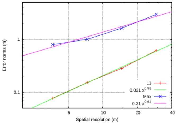
A quantitative assessment of the quality of the numerical solution is given in Fig. 3. The average (L1-norm) and max-imum errors att=220 s are computed as
kek1=
P
i1i|yi−y(xi)|
P
i1i
kekmax=max
i |yi−y(xi)|
where(xi,yi)is the discrete numerical solution for the wave profile,y(xi)is the (interpolated) analytical solution at po-sition xi and 1i is the (variable) grid size. The average norm shows first-order convergence and the maximum er-ror slightly less than first-order convergence. This is not unexpected given that errors are dominated by the contact discontinuities at the wet-dry transition, where the Godunov scheme (or any other shock-capturing scheme) reduces to first-order accuracy. From a tsunami modelling perspective, this test case demonstrates that, even for very simple coast-line geometries, spatial resolutions of less than a few tens of metres are necessary to accurately capture wave runup and inundation on the shoreline. All the data necessary to repro-duce this test case are given on the Gerris web site (Popinet, 2011a).
4 Results for the Tohoku tsunami
0
1
3
4 2
Fig. 1. An example of quadtree discretisation (left) together with its logical representation (right). The level of the cells in the tree are also
given.
-25 -20 -15 -10 -5 0 5 10 15 20
-200 0 200 400 600 800 1000
y (m)
x (m)
beach t = 160 sec t = 175 sec t = 220 sec
Fig. 2. Topography, analytical (lines) and numerical (symbols)
wave profiles for the times indicated in the legend. The numeri-cal results are forlmax=14 i.e. a maximum spatial resolution of ≈3.6 m. The numerical solution is represented using only one in every six discretisation points for clarity.
0.1 1
5 10 20 40
Error norms (m)
Spatial resolution (m)
L1 0.021 x0.99 Max 0.31 x0.64
Fig. 3. Convergence of the average and maximum errors with
spa-tial resolution. The errors are for the predicted wave profile at t=220 s.
Fig. 4. Extent of the simulation domain and bathymetry (altitude
in metres). DART buoys (black labels) and GLOSS stations (red labels).
(for the Japanese islands only). Both datasets are stored us-ing the 2d-tree (KDT) hierarchical terrain database system of Gerris with on-disk storage sizes of:
• GEBCO 08: global dataset, 933 million points, 21 GBytes, KDT index: 65 MBytes
• SRTM, 3 arc-s: Japan only, 58 million points, 1.4 GBytes, KDT index: 4.1 MBytes
These on-disk datasets are accessed during the simulation to reconstruct the bathymetry as required as the spatial reso-lution evolves. The size of the KDT index gives an order of magnitude estimate of the amount of dynamic memory (RAM) required to access each dataset.
Fig. 5. Initial vertical displacement (metres) derived from the
sub-faults model of Shao, Li and Ji, UCSB (Preliminary model III). The location of wave buoys (801–807) and bottom pressure gauges records (TM1 and TM2 located between TM1 and 802) used in this study are also indicated.
the source model using the DART buoys and tide gauges data, and also that, in a realtime forecasting scenario, using only seismic information may allow a quicker estimate of the source (because seismic waves travel faster than gravity waves).
Several deformation models for the Tohoku earth-quake have been made available by the seismic research community, and some of them were released only a few hours after the event. A selection of such models is avail-able on the USGS Tohoku web site (USGS, 2011). Differ-ent methods can be used for the seismic inversion (combined with different weighting for the various seismic datasets) and the scatter in the resulting predicted deformations can be large. For this study I have used one of the deformation mod-els obtained by Shao, Li and Ji, UCSB, more precisely their preferred “Preliminary model III” released on 14 March 2011 (Shao et al., 2011). This model predicts vertical deformations which are significantly larger than any of the other models mentioned on the USGS Tohoku web site and was the only source model I tested which resulted in satisfying agreement with tsunami wave measurements. The initial vertical wave elevation was assumed to be equal to the total vertical bot-tom displacement predicted by the source model. This dis-placement was obtained by superposition of the 190 Okada subfaults displacements used in the seismic inversion. The fault model also includes the relative rupturing times of each subfault, but I chose to assume that the total rupturing time (3 min) was small enough to be negligible. The resulting ini-tial vertical displacement is illustrated in Fig. 5.
For the adaptive model, the choice of spatial resolution is very flexible and can be based on several simultaneous cri-teria, depending on which specific information one would like to extract from the model. In this study I chose to
illus-trate how adaptivity can help obtain simultaneous solutions for two aspects of tsunami modelling which are generally considered as conflicting in term of resolution requirements: long-distance propagation and detailed inundation/damage predictions. In this study, both regimes are captured using a single criterion but different maximum spatial resolutions: the mesh size1is adapted so that
|∇h|1 < ǫ (4)
whereǫ is a control parameter set to 2.5 cm. ǫ can be in-terpreted as the maximum truncation error in the free surface elevation of a spatially first-order discretisation scheme. This corresponds to the maximum error expected near sharp dis-continuities (i.e. shocks). In smooth regions, the scheme is second-order and errors will be significantly smaller. There are primarily two regions where one can expect larger dis-cretisation errors: wave fronts and “breaking” waves in shallow water i.e. the two regimes of long-distance wave propagation and inundation we are interested in. I have shown in a previous study that adequate propagation of long-wave energy over large distances with the non-linear, shock-capturing numerical scheme requires spatial resolutions of the order of one arc-minute in order to minimise numerical wave dissipation (Popinet, 2011c). Following this, the max-imum resolution for deep water wave propagation is set to 12 levels of quadtree refinement, giving a maximum deep water resolution of close to 1 arc-min (which is also com-parable to the spatial resolution of the deep water GEBCO bathymetry). Detailed inundation modelling, on the other hand often requires higher spatial resolution, in order to cap-ture fine-scale topographic effects as well as wave runup (see the previous section). In this study the maximum resolution of “inundable areas” (any part of the domain above sea level) is set to 15 levels of refinement (or 8 arc-s, or≈250 m) which is comparable to the spatial resolution of the SRTM topo-graphic dataset. Note that this choice of adaptive refinement does not rely on any a priori assumptions on the location of inundated areas and/or propagation of the tsunami wave and could thus be applied to any other event. The variable resolution is also used to implement “sponge layers” on the open boundaries of the domain. Within bands approximately 3.65 degrees wide along all four boundaries of the domain, the spatial resolution is coarsened to only 5 levels (approxi-mately 2.3◦resolution). The resulting numerical dissipation
dampens waves before they exit the domain, thus minimising spurious wave reflections at boundaries.
by the tsunami. The detail shown covers an area of roughly 220×180 km.
Figure 8 gives the corresponding evolution in the total number of grid points over 10 h of modelled physical time. The initial number of grid points is approximately 50 000 which corresponds to the number of elements necessary to resolve the source of Fig. 5 with the accuracy specified by Eq. (4). After a rapid initial increase, the number of grid points reaches a maximum of approximately one million at
t=5 h, the time at which waves start exiting the compu-tational domain. This can be compared with 224, the total number of grid points which would be necessary if the whole domain was resolved at a constant resolution of≈1 arc-min (the resolution necessary to model deep-water wave propa-gation correctly), as well as an upper bound of 230≈ one billion, if the whole domain was resolved at the maximum inundation resolution of 8 arc-s. A somewhat more realis-tic upper bound can be estimated by assuming that a starealis-tic “nested mesh” approach could be used to resolve only low-lying (altitude less than e.g. 50 m) emerged land areas at the maximum resolution (8 arc-s) and the rest of the domain at a resolution of one arc-minute. This still gives about 50 million grid points, so that a fair estimate of the gain in number of grid points obtained with the adaptive method for this par-ticular simulation is a factor of order 15 to 50. Note also that this factor is scale-dependent, so that as pointed out in Popinet (2011c) it will increase with increasing maximum spatial resolution. The gain in runtime is more difficult to estimate as it depends on the details of the respective imple-mentations and optimisations of different methods. Previous comparisons show that the current quadtree implementation in Gerris is roughly five times slower than a comparable nu-merical scheme implemented on a regular Cartesian grid so that the gain in runtime would be a factor from 3 to 10. Note however that this also assumes that the speed of the regu-lar Cartesian grid scheme would not be affected by the regu-large memory requirements, which is unlikely in practice. The results presented here were obtained on a single-processor standard desktop PC with an average runtime of roughly two hours for one hour of physical time (this ratio is much lower in the initial phases of the simulation where few grid points are used). This runtime could be decreased by using the par-allel capabilities of Gerris (including dynamic parpar-allel load-balancing) (Agbaglah et al., 2011).
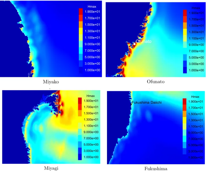
A general overview of the maximum wave elevation reached over 10 h is given in Figs. 9, 10 and 11. Maxi-mum wave elevations in excess of 40 m are predicted along the coast of the Oshika peninsula (Fig. 11-Miyagi). These extreme values extend to the north of Ofunato, roughly be-tween latitudes 38◦N and 39.5◦N. Large values are other-wise predicted along the Japanese coast from 35◦N to 42◦N (Fig. 10). Offshore, the maximum amplitude is reached along an east-south-east direction with strong modulations due to the many small submerged and emerged topographic features in the Pacific (Fig. 9).
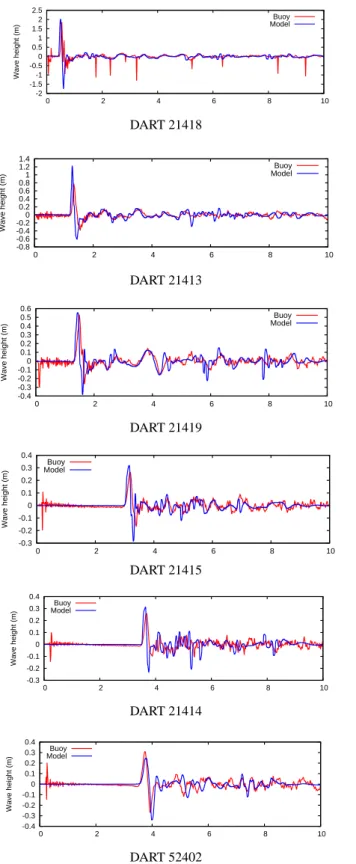
A first validation of the model is obtained by comparing the modelled wave elevation timeseries with observed sea level at DART buoys locations. Figure 12 illustrates these timeseries for all the DART buoys deployed in the simulation domain (see Fig. 9) which were active during the event and which measured deviations larger than 10 cm. The DART timeseries were obtained directly from the raw data avail-able in real-time on the DART website (NOAA, 2011) and were low-pass filtered via Fourier decomposition to remove the tidal components. The model correctly predicts both the arrival times and maximum wave elevations at all lo-cations (keeping in mind that DART observations were not used to constrain the source model). The initial wave front is steeper than observed for most stations however. This was also observed in a previous study (Popinet, 2011c) and may be due to excessive anti-diffusion of the limiter in the shock-capturing scheme. It is also clear that the model reproduces many of the high-frequency, secondary wave reflections. For example, the clear modelled and measured signal around
t=4 h for DART 21419 is most likely due to the reflection of the primary wave off the Emperor seamount chain (the underwater range extending south-east from DART 21416 in Fig. 4).
While the DART buoys data validate the long-distance, deep-water propagation, tidal gauges can give information on the inshore wave propagation. In this study, I chose to use only data available within the Global Sea Level Observing System (GLOSS) (IOC, 2011b). The GLOSS database sys-tem provides a unified way to access hundreds of sea level recording systems, in near real-time, which greatly simpli-fies the implementation of an automated tsunami forecasting system. Unfortunately, many existing tide gauges have not been integrated within GLOSS yet. For the area I consider only six sites are available for the Japanese islands. Another limitation of the GLOSS database is that the location of tide gauges is only recorded with an accuracy of one arc-minute. This can easily lead to tide gauges being incorrectly located in “dry” areas of the numerical model. For this study the lo-cations of gauges have been adjusted to their most probable locations based on bathymetry and satellite images.
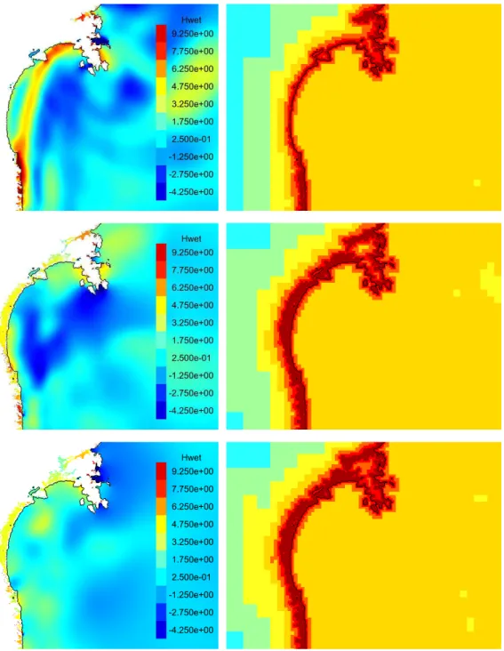
Fig. 6. Wave evolution over most of the modelled domain. Rows from top to bottom,t=1,2,4 h. Left column: evolution of wave elevation, dark blue<−1 m, dark red>2 m. Right column: corresponding evolution of spatial resolution, dark blue 5 levels,≈2.3◦, yellow 12 levels,
≈1 arc-min, dark red 15 levels,≈8 arc-s,≈250 m.
measured a positive first wave before ceasing transmission at
t≈30 min. The model predicts a negative first wave which is clearly related to the negative initial amplitude distribution of the source model (Fig. 5).
The characteristics of the following waves are very site-specific but can be roughly classified according to their dom-inant frequency. Some sites such as Hanasaki or Ishigaki-jima have dominant waves at relatively long periods (≈1 h)
Fig. 7. Detail of the wave evolution in the Miyagi prefecture area. The black line in all figures is the coastline. Rows from top to bottom,
t=1,2,4 h. Left column: evolution of wave elevation (colorbar in metres). Right column: corresponding evolution of spatial resolution, yellow 12 levels≈1 arc-min, dark red 15 levels≈8 arc-s≈250 m.
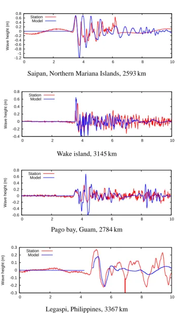
the detailed geometry of the harbour is crucial in determining the amplification of short-period components. This could explain the under-estimation of wave amplitudes for these sites. Finally, the sites at Wake island and Pago bay are characterised by very high frequencies (periods smaller than 15 min). Both the characteristic frequencies and amplitudes of the measured waves are well captured by the model. Both sites are located on small, isolated islands surrounded
10000 100000 1e+06 1e+07 1e+08 1e+09 1e+10
0 2 4 6 8 10
Number of grid points
Time (hours) adaptive
224 230
Fig. 8. Evolution with physical time of the total number of grid
points.
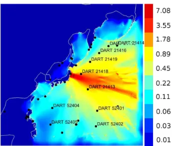
Fig. 9. Maximum wave elevation reached over 10 h. The
(logarith-mic) colorbar gives the maximum wave elevation in metres. The low values close to the boundaries of the domain are due to the mesh coarsening used to limit spurious wave reflections.
Prediction of the extent of tsunami inundation as a func-tion of detailed topography is an important aspect of tsunami modelling, particularly when used for urban planning and risk assessment. Extensive survey work after the Tohoku tsunami done in very difficult conditions by the Tohoku Earthquake Tsunami Joint Survey Group (TTJT, 2011b,a; Mori et al., 2011) as yielded an impressive amount of data on this event: more than 5000 individual GPS records of wave height have been collected along the entire eastern Japanese coastline. In addition to this field data, various satellites have also recorded different aspects of the tsunami, including
de-Fig. 10. Detail of the maximum wave elevation reached over 10 h.
The (logarithmic) colorbar gives the maximum wave elevation in metres. The model predict maximum wave elevations of more than 40 m on the coast of the Oshika peninsula (south of Ofunato).
tailed maps of the extent of flooding one day after the event. Figure 15 (left) displays a detail of the topography contours (red), survey data points (blue) and extent of flooding (green) estimated using analysis of high-resolution Synthetic Aper-ture Radar (SAR) imaging (DLR, 2011) for the Miyagi pre-fecture area.
In the southern half of the map, the flooding extent is clearly controlled by the relatively steep topography, and less so for the northern half. Figure 15 (right) shows a compar-ison between the satellite estimation of the flooding extent on 12 March with both the modelled maximum extent of the tsunami (green) and the modelled inundated area (depth larger than 10 cm) att=10 h (black). Both sets of curves are a satisfactory approximation of the satellite data, with the maximum extent curve (green) lying beyond the satellite data as expected, and the 10 cm flooding curve (black) gen-erally underestimating slightly the extent of flooding com-pared with the satellite estimate. These curves are available as Google Earth KML files for the entire simulation domain of Fig. 4 (Popinet, 2011b) and can thus be compared visu-ally with satellite images of the damaged areas. This also confirms the good model predictions of the extent of tsunami damage.
Miyako
Ofunato
Miyako
Miyagi
Ofunato
Fukushima
Fig. 11. Details of maximum wave elevation reached over 10 h. The colorbar gives the the maximum wave elevation in metres. Values larger
than 19 m are obtained along the coast of the Oshika peninsula (Miyagi) and Ofunato.
between 36 and 37.5◦N as well as north of 42◦N (on the coast of Hokkaido where the Hanasaki tide gauge is located, Fig. 13). The extreme wave elevations (peak values in ex-cess of 40 m) observed between 38.5 and 40.5◦N are also captured by the model with the correct amplitudes, but the modelled extremes occur about one degree south of the ob-served values: this corresponds to the Ofunato and Miyako regions respectively (see Fig. 11). Both regions are charac-terised by very steep and indented coastlines which, together with proximity to the source, explains the high wave eleva-tions reached there. The sources of error for both datasets (surveyed and modelled) are of course different: the model will suffer from a representation bias due for example to the inaccurate representation of steep terrain (even at the maxi-mum resolution of 250 m); while the surveyed data is likely to suffer from a sampling bias due to the difficulty of survey-ing every location and/or due to particular choices in the
sam-pling procedure (e.g. focusing on tsunami damage to infras-tructure etc...). Such a sampling bias could explain the dis-crepancy between modelled and surveyed data for the Miyagi area (corresponding to the inundation maps of Fig. 15). The surveyed data for this area seems to be biased low (with many samples even reporting negative wave elevations) while the modelled elevation distribution seem to be more consistent with the observed extent of inundation.
-2 -1.5 -1 -0.5 0 0.5 1 1.5 2 2.5
0 2 4 6 8 10
Wave height (m)
Buoy Model DART 21418 -0.8 -0.6 -0.4 -0.2 0 0.2 0.4 0.6 0.8 1 1.2 1.4
0 2 4 6 8 10
Wave height (m)
Buoy Model DART 21413 -0.4 -0.3 -0.2 -0.1 0 0.1 0.2 0.3 0.4 0.5 0.6
0 2 4 6 8 10
Wave height (m)
Buoy Model DART 21419 -0.3 -0.2 -0.1 0 0.1 0.2 0.3 0.4
0 2 4 6 8 10
Wave height (m)
Buoy Model DART 21415 -0.3 -0.2 -0.1 0 0.1 0.2 0.3 0.4
0 2 4 6 8 10
Wave height (m)
Buoy Model DART 21414 -0.4 -0.3 -0.2 -0.1 0 0.1 0.2 0.3 0.4
0 2 4 6 8 10
Wave height (m)
Buoy Model
DART 52402
Fig. 12. Timeseries of observed and modelled wave height at DART
buoys locations, ordered by increasing arrival time from top to bot-tom. Horizontal axis is time in hours.
-15 -10 -5 0 5 10 15 20 25
0 2 4 6 8 10
Wave height (m)
Station Model
Ofunato, Japan, 99 km
-2 -1.5 -1 -0.5 0 0.5 1 1.5 2 2.5 3
0 2 4 6 8 10
Wave height (m)
Station Model
Hanasaki, Japan, 588 km
-1.5 -1 -0.5 0 0.5 1 1.5
0 2 4 6 8 10
Wave height (m)
Station Model
Omaezaki, Japan, 581 km
-0.6 -0.4 -0.2 0 0.2 0.4 0.6 0.8
0 2 4 6 8 10
Wave height (m)
Station Model
Naha, Okinawa, Japan, 1950 km
-0.3 -0.2 -0.1 0 0.1 0.2 0.3
0 2 4 6 8 10
Wave height (m)
Station Model
Ishigaki-jima, Japan, 2344 km
Fig. 13. Measured and modelled timeseries at GLOSS stations
loca-tions. Horizontal axis is time in hours. Distances from the epicentre are indicated in the legends.
-1.2 -1 -0.8 -0.6 -0.4 -0.2 0 0.2 0.4 0.6 0.8
0 2 4 6 8 10
Wave height (m)
Station Model
Saipan, Northern Mariana Islands, 2593 km
-0.4 -0.2 0 0.2 0.4 0.6 0.8
0 2 4 6 8 10
Wave height (m)
Station Model
Wake island, 3145 km
-0.6 -0.4 -0.2 0 0.2 0.4 0.6 0.8
0 2 4 6 8 10
Wave height (m)
Station Model
Pago bay, Guam, 2784 km
-0.3 -0.2 -0.1 0 0.1 0.2 0.3
0 2 4 6 8 10
Wave height (m)
Station Model
Legaspi, Philippines, 3367 km
Fig. 14. Measured and modelled timeseries at GLOSS stations
loca-tions (continued). Horizontal axis is time in hours. Distances from the epicentre are indicated in the legends.
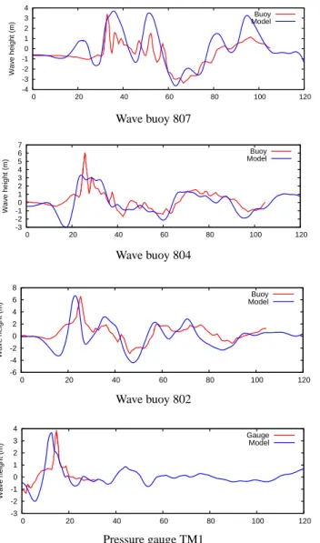
model may be locally inaccurate: the observed first wave is positive whereas the modelled first wave is negative (with an amplitude of−5 m) which is consistent with the large nega-tive amplitude area of the source model west of the epicentre. To try to clarify this issue, the model output is compared in Figs. 17 and 18 with wave height records from a further six wave buoys and two bottom pressure gauges located a few tens of kilometres offshore the Sanriku coastline (locations indicated on Fig. 5). An obvious discrepancy is that all the modelled timeseries show a large negative first (or second) wave which is absent in the field records. As noted before for the Ofunato tide gauge, this is consistent with the large negative amplitude in the source model (south of TM1 in Fig. 5). For most sites, the peak amplitude of the largest pos-itive wave (and subsequent waves) is correctly captured by the model with the notable exceptions of buoys 804, 803 and
801. The peak wave amplitude is under-estimated by a factor of two for buoy 804 and over-estimated by a similar factor at buoys 803 and 801. This is consistent with the bias in predicted wave elevations of Fig. 16: buoys 803 and 801 are located offshore the Ofunato region (positive bias) whereas buoy 804 is located offshore the Miyako region (negative bias). This confirms that the biases in predicted wave ele-vations on the coastline are likely due to local errors in the source model rather than an inaccurate representation of the dynamics of flooding on this steep terrain.
Note also that several other source models proposed for this event suffer from a similar north-south bias. Using for example the source model proposed by Fuji et al. (2011), based on inversion of tide and pressure gauges and wave buoys (including all the sites of Figs. 17 and 18) still leads to a large under-prediction of the wave amplitude and runup in the Miyako region (but does reduce the amplitude in the Ofunato region). Petukhin et al also report a very similar bias for their source model based purely on seismic inversion (see Fig. 3 of Petukhin et al., 2011) and suggest that this may be due to an inaccurate representation of the bathymetry for this area. Based on the results presented here, I do no think that this is a sufficient explanation since both the northern and southern parts of the Sanriku coast are described with simi-lar datasets and do not differ markedly in term of complexity. The discrepancy is more likely due to the interaction of the main wave – which looks correctly described given the agree-ment with far-field measureagree-ments – with the initial wave field between the epicentre and the coast.
5 Conclusions
The quadtree-adaptive Saint-Venant solver implemented within Gerris was shown to provide robust and accurate so-lutions for the full range of wave phenomena associated with the Tohoku tsunami. The adaptive spatial resolution ranged from approximately 250 m to 250 km for a domain spanning 73◦of latitude and longitude. The maximum spa-tial resolution proved adequate to resolve inundation pro-cesses in most areas while adaptivity allowed to track deep-water wave fronts at a typical resolution of 1 arc-min (≈ 1.8 km) which was sufficient to ensure good long-distance wave energy conservation. A conservative estimate of the gain in computational efficiency obtained with the adaptive model is a factor of ten compared to a discretisation using a spatially-variable but constant-in-time resolution. This es-timate increases to several orders of magnitude when com-pared to simple, spatially-constant (e.g. Cartesian) discreti-sations. Furthermore, as pointed out in Popinet (2011c) this gain is scale-dependent and will increase with maximum spa-tial resolution. The criteria used for adaptive mesh refine-ment are simple and do not rely on a priori assumptions about the solution. They are thus applicable to any tsunami event.
Fig. 15. Maps of inundation extent for the Miyagi prefecture area. Left: 0 and 10 m contours (red), SAR estimate of inundation extent on
12 March 2011 (green), field survey data points (blue). Right: SAR inundation estimate (green), maximum modelled inundation extent (red) and modelled inundated areas att=10 h (black).
Fig. 16. Wave elevation reached as a function of latitude. For each
dataset (modelled and surveyed) the curve is the median elevation in each 0.2◦-wide bin, and the shaded areas delimit the lower and upper quartiles of the wave elevation distribution. The vertical lines indicate the different regions displayed in Fig. 11.
of the subsequent wave evolution. The source model of Shao, Li and Ji was shown to lead to remarkably accurate predictions of initial wave amplitudes and arrival times as well as subsequent multiple reflections from bathymetry for all the DART buoys located within the simulation domain. Shao, Li and Ji only used information on seismic waves for their source inversion, so that comparisons between the mod-elled and observed surface waves are a true independent val-idation of both source and tsunami model consistency. This study demonstrates that accurate and consistent source mod-els for tsunami wave propagation can be constructed using seismic waves only. Coupled with the high level of automa-tion readily possible with the adaptive model, this opens the door to realtime forecasting of tsunami propagation and inun-dation, where the main time constraint is related to acquisi-tion and processing of the fast (a few km s−1) seismic waves signals rather than the slower (a few hundreds of m s−1) sur-face gravity waves signals.
-4 -3 -2 -1 0 1 2 3 4
0 20 40 60 80 100 120
Wave height (m)
Buoy Model
Wave buoy 807
-3 -2 -1 0 1 2 3 4 5 6 7
0 20 40 60 80 100 120
Wave height (m)
Buoy Model
Wave buoy 804
-6 -4 -2 0 2 4 6 8
0 20 40 60 80 100 120
Wave height (m)
Buoy Model
Wave buoy 802
-3 -2 -1 0 1 2 3 4
0 20 40 60 80 100 120
Wave height (m)
Gauge Model
Pressure gauge TM1
Fig. 17. Comparison between recorded and modelled wave
ampli-tudes for the inshore locations indicated in Fig. 5. The stations are ordered by latitude from top to bottom. The horizontal axis is time in minutes.
All stations show satisfactory agreement when allowing for the well-known dependencies of in-shore signals on (unresolved) topographic details such as breakwaters. Model results also compare well with satellite estimates of the extent of flooding as well as with extensive point survey data along the eastern Japanese coastline. However, there is a significant discrepancy between surveyed and modelled wave elevations on the Sanriku coastline, where extreme wave elevations (up to 40 m) were observed. These extremes values are reproduced in the model but further south than observed. Analysis of further inshore wave buoys and pressure gauge records indicate that this discrepancy is most probably due to an incorrect incoming wave rather than inaccurate modelling of inundation on the complex
-3 -2 -1 0 1 2 3 4 5
0 20 40 60 80 100 120
Wave height (m)
Gauge Model
Pressure gauge TM2
-4 -2 0 2 4 6 8 10 12
0 20 40 60 80 100 120
Wave height (m)
Buoy Model
Wave buoy 803
-6 -4 -2 0 2 4 6 8 10 12 14
0 20 40 60 80 100 120
Wave height (m)
Buoy Model
Wave buoy 801
-1.5 -1 -0.5 0 0.5 1 1.5 2 2.5
0 20 40 60 80 100 120
Wave height (m)
Buoy Model
Wave buoy 806
Fig. 18. Comparison between recorded and modelled wave
ampli-tudes for the inshore locations indicated in Fig. 5 (continued). The stations are ordered by latitude from top to bottom. The horizontal axis is time in minutes.
and steep shoreline. A similar discrepancy has been noted by other authors, using different source models (Fuji et al., 2011; Petukhin et al., 2011). This may indicate that our understanding of the local seafloor deformations during the Tohoku earthquake is incomplete. A potential mechanism which could explain the discrepancy is the occurence of local submarine landslides, (i.e. plastic rather than elastic deformations), triggered by the earthquake.
Edited by: S. Tinti
References
Abe, K.: Synthesis of a tsunami spectrum in a semi-enclosed basin using its background spectrum, Pure Appl. Geophysics, 168, 1101–1112, 2011.
Agbaglah, G., Delaux, S., Fuster, D., Hoepffner, J., Josserand, C., Popinet, S., Ray, P., Scardovelli, R., and Zaleski, S.: Par-allel simulation of multiphase flows using octree adaptivity and the volume-of-fluid method, Compte-rendus de l’Acad´emie des Sciences, Paris, 339, 194–207, http://gfs.sf.net/papers/ agbaglah2011.pdf, 2011.
Audusse, E., Bouchut, F., Bristeau, M.-O., Klein, R., and Perthame, B.: A fast and stable well-balanced scheme with hydrostatic re-construction for shallow water flows, SIAM J. Sci. Comp, 25, 2050–2065, 2004.
Bentley, J. and Friedman, J.: Data structures for range searching, ACM Computing Surveys (CSUR), 11, 397–409, 1979. Carrier, G., Wu, T., and Yeh, H.: Tsunami run-up and draw-down
on a plane beach, J. Fluid Mech., 475, 25, 2003.
Center for Satellite-Based Crisis Information: Disaster Extent Map – Japan – Sendai Region, http://www.zki.dlr.de/map/1950, 2011. de Saint-Venant, A. B.: Th´eorie du mouvement non-permanent des eaux, avec application aux crues des rivi`eres et `a l’introduction des mar´ees dans leur lit, CR Acad. Sci. Paris, 73, 147–154, 1871. Fuji, Y., Satake, K., Sakai, S., Shinohara, M., and Kanazawa, T.: Tsunami source of the 2011 off the Pacific coast of Tohoku, Japan earthquake, Earth Planets Space, 63, 815–820, 2011. George, D. and LeVeque, R.: High-resolution methods and adaptive
refinement for tsunami propagation and inundation, Hyperbolic Problems: Theory, Numerics, Applications, 541–549, 2008. Grilli, S., Ioualalen, M., Asavanant, J., Shi, F., Kirby, J., and Watts,
P.: Source constraints and model simulation of the December 26, 2004, Indian Ocean Tsunami, J. Waterw. Port. C-Asce, 133, 414–428, 2007.
Harig, S., Pranowo, W., and Behrens, J.: Tsunami simulations on several scales, Ocean Dynam., 58, 429–440, 2008.
IOC: General Bathymetric Chart of the Oceans, http://www.gebco. net/data and products/gridded bathymetry data, 2011.
IOC: Global Sea Level Observing System, http://www.
gloss-sealevel.org, 2011.
Liang, Q. and Borthwick, A.: Adaptive quadtree simulation of shal-low fshal-lows with wet-dry fronts over complex topography, Comput. Fluids, 38, 221–234, 2009.
Liang, Q., Borthwick, A., and Stelling, G.: Simulation of dam-and dyke-break hydrodynamics on dynamically adaptive quadtree grids, Int. J. Numer. Meth. Fl., 46, 127–162, 2004.
Liu, P.: The Third International Workshop on Long-Wave Runup Models, http://isec.nacse.org/workshop/2004 cornell, 2004. Miller, G. R.: Relative spectra of tsunami, Hawaii Inst. Geophys.,
Univ. Hawaii, 72, 1–6, 1972.
Mori, N., Takahashi, T., Yasuda, T., and Yanagisawa, H.: Survey of 2011 Tohoku earthquake tsunami inundation and run-up, Geo-phys. Res. Lett., 38, doi:10.1029/2011GL049210, 2011. NASA: Space Shuttle Radar Topography Mission, http://www2.jpl.
nasa.gov/srtm, 2011.
NOAA: National Data Buoy Center – DART, http://www.ndbc. noaa.gov/dart.shtml, 2011.
Petukhin, A., Yoshida, K., and Miyakoshi, K.: Simulation of tsunami and long-period ground motions during the M9.0 2011 Tohoku-oki earthquake, in: Japan Geoscience Union meeting, 2011.
Popinet, S.: Gerris: a tree-based adaptive solver for the incompress-ible Euler equations in complex geometries, J. Comput. Phys., 190, 572–600, http://gfs.sf.net/gerris.pdf, 2003.
Popinet, S.: The Gerris Flow Solver, http://gfs.sf.net, 2003–2012. Popinet, S.: An accurate adaptive solver for surface-tension-driven
interfacial flows, J. Comput. Phys., 228, 5838–5866, http://gfs. sf.net/papers/tension.pdf, 2009.
Popinet, S.: Gerris – Oscillations in a parabolic container test case, http://gerris.dalembert.upmc.fr/gerris/tests/tests/parabola. html, 2010.
Popinet, S.: Gerris – Monai tsunami benchmark, http://gerris. dalembert.upmc.fr/gerris/examples/examples/monai.html, 2010. Popinet, S.: Gerris – The 2004 Indian Ocean tsunami, http://gerris.
dalembert.upmc.fr/gerris/examples/examples/tsunami.html, 2010.
Popinet, S.: Gerris – Tsunami runup onto a plane beach test case, http://gerris.dalembert.upmc.fr/gerris/tests/tests/shore. html, 2011.
Popinet, S.: Gerris simulations of the 11th March Japanese tsunami, http://gfs.sourceforge.net/wiki/index.php/11th March Japanese tsunami, 2011.
Popinet, S.: Quadtree-adaptive tsunami modelling, Ocean Dynam-ics, 61, 1261–1285, http://gfs.sf.net/papers/tsunami.pdf, 2011. Popinet, S. and Rickard, G.: A tree-based solver for adaptive ocean
modelling, Ocean Modell., 224–249, http://gfs.sf.net/ocean.pdf, 2007.
Popinet, S., Gorman, R. M., Rickard, G. J., and Tolman, H. L.: A quadtree-adaptive spectral wave model, Ocean Modell., 34, 36– 49, http://gfs.sf.net/papers/wave.pdf, 2010.
Shao, G., Li, X., and Ji, C.: Preliminary Result of the Mar 11, 2011 Mw 9.1 Honshu Earthquake, http://www.geol.ucsb.edu/faculty/ ji/big earthquakes/2011/03/0311 v3/Honshu.html, 2011. Takahashi, R. and Aida, I.: Spectra of several tsunamis observed on
the coast of Japan, Bull. Earth. Res. Inst., 41, 299–314, 1963 in Japanese.
Third international workshop on long-wave runup models: Tsunami runup onto a plane beach, http://isec.nacse.org/workshop/2004 cornell/bmark1.html, 2004.
The 2011 Tohoku Earthquake Tsunami Joint Survey Group: A unified data set off the northeastern Pacific Ocean, http://www. coastal.jp/ttjt/, release 20111110, 2011.
The 2011 Tohoku Earthquake Tsunami Joint Survey Group: Na-tionwide Field Survey of the 2011 Tohoku Earthquake Tsunami off the Pacific Coast, Journal of Japan Society of Civil Engineers, Series B (B2 JSCE (Coastal Eng.)), 67, 63–66, 2011.
USGS: Mw 9.0 Earthquake Offshore Honshu, Japan – Finite Fault Model, http://earthquake.usgs.gov/earthquakes/eqinthenews/ 2011/usc0001xgp/finite fault.php, 2011.