Quasi 2D hydrodynamic modelling of the flooded hinterland due to dyke breaching on the Elbe River

www.adv-geosci.net/11/21/2007/ © Author(s) 2007. This work is licensed under a Creative Commons License.

Geosciences

Quasi 2D hydrodynamic modelling of the flooded hinterland due to

dyke breaching on the Elbe River

S. Huang, S. Vorogushyn, and K.-E. Lindenschmidt

GFZ GeoForschungsZentrum Potsdam, Section 5.4 – Engineering, Hydrology, Telegrafenberg, 14473 Potsdam, Germany Received: 15 December 2006 – Revised: 5 April 2007 – Accepted: 4 May 2007 – Published: 16 May 2007

Abstract. In flood modeling, many 1D and 2D combina-tion and 2D models are used to simulate diversion of wa-ter from rivers through dyke breaches into the hinwa-terland for extreme flood events. However, these models are too de-manding in data requirements and computational resources which is an important consideration when uncertainty anal-ysis using Monte Carlo techniques is used to complement the modeling exercise. The goal of this paper is to show the development of a quasi-2D modeling approach, which still calculates the dynamic wave in 1D but the discretisation of the computational units are in 2D, allowing a better spa-tial representation of the flow in the hinterland due to dyke breaching without a large additional expenditure on data pre-processing and computational time. A 2D representation of the flow and velocity fields is required to model sediment and micro-pollutant transport. The model DYNHYD (1D hydro-dynamics) from the WASP5 modeling package was used as a basis for the simulations. The model was extended to incor-porate the quasi-2D approach and a Monte-Carlo Analysis was used to conduct a flood sensitivity analysis to determine the sensitivity of parameters and boundary conditions to the resulting water flow. An extreme flood event on the Elbe River, Germany, with a possible dyke breach area was used as a test case. The results show a good similarity with those obtained from another 1D/2D modeling study.

1 Introduction

Hydrodynamic models are important for the simulation and prediction of inundation processes due to dyke breaching during flood events. An array of models of varying com-plexity levels may be used. Following a categorization in the number of spatial dimensions, simulations are often carried

Correspondence to:K.-E. Lindenschmidt (kel@gfz-potsdam.de)

out using one-dimensional (1D) or two-dimensional (2D) models. 1D hydrodynamic models often solve the St.Venant full dynamic wave equations which respect to both momen-tum and mass continuity of water transport through a meshed system. 2D models are based on shallow water equations to describe the motion of water (for examples, see D’Alpaos et al., 1994 and Chua et al., 2001). A combination of both 1D and 2D approaches have also been used in which the flow in the main river channel is solved in 1D and the overbank inundated areas are solved in 2D using the diffusive wave equation or storage cells (for examples, see Bates and De Roo, 2000; Han et al., 1998 and Vorogushyn et al., 2007). 2D and 1D/2D combination models are generally computa-tionally more extensive and have more requirements on input data and pre-processing than 1D models. This is particularly a concern when automated methods for parameter optimiza-tion or Monte-Carlo methods for uncertainty analysis are to be implemented. However, 1D models are not sufficient to describe the spatial variability of water depths, velocities and flows in floodplains, polders and other overbanked inundated areas during flood events.

Hence, a quasi-2D approach using a 1D hydrodynamic model is proposed that allows its discretisation to be ex-tended into the hinterland giving a 2D representation of the inundation area (see Fig. 1). Aureli et al. (2006) have used quasi-2D numerical modeling adopting the hydrodynamic module of the software DHI-Mike 11. We also compared the results of a dyke breach and hinterland inundation obtained from a quasi-2D model and a fully-2D finite volume model and found good agreement between them in the simulation results.

Fig. 1. 1D hydrodynamic channel-junction (link-node) network allowing a 2D spatial representation of overbank inundated areas (source: Ambrose et al., 1993).

Table 1. Discharge statistics for the gages at Torgau and Luther-stadt Wittenberg (MQ – mean discharge, MHQ – mean maxi-mum annual flood, HQ – highest recorded flood event); source: Gew¨asserk¨undliches Jahrbuch, Elbegebiet Teil 1, 2003.

Gage Elbe-km Series MQ MHQ HQ (date) Torgau 154.2 1936 - 2003 344 1420 4420 (18.08.2002) L. Wittenberg 214.1 1961 - 2003 369 1410 4120 (18.08.2002)

Discharge (m3/s)

α

computational network. This model is discretised to the hin-terland representing the inundation area. Monte-Carlo Anal-yses were carried out to analyze globally the sensitivity of selected parameters and boundary conditions on state vari-ables. The analysis also indicates good model stability for a wider range of parameter settings and boundary conditions and the model’s applicability to other test sites.

2 Methods

2.1 Hydrodynamic model DYNHYD

This description of the model DYNHYD has been drawn from Ambrose et al. (1993), Lindenschmidt et al. (2005) and Lindenschmidt (2007)1, however, a short excerpt is war-ranted here. In DYNHYD a river is discretised using a “channel-junction” scheme. The channels have

rectangu-1_{Lindenschmidt, K.-E.: Quasi-2D approach in modelling the}

transport of contaminated sediments in floodplains during river flooding – model coupling and uncertainty analysis, Environmen-tal Engineering Sciences, in review, 2007.

∂t ∂x

whereaf is the frictional acceleration,agis the gravitational acceleration along the longitudinal axisx,Uis the mean ve-locity,∂U/∂tis the local inertia term, or the velocity rate of change with respect to timetandU ∂U/∂xis the convective inertia term, or the rate of momentum change by mass trans-fer. The junctions calculate the storage of water described by the continuity equation:

∂H ∂t =

1 B ·

∂Q

∂x (2)

whereB is the channel width, H is the water surface ele-vation (head), ∂H /∂t is the rate of water surface elevation change with respect to timet, and∂Q/∂xis the rate of water volume change with respect to distancex. The dischargeQis additionally related to river morphology and bottom rough-ness using Manning’s equation:

Q=r 2/3

H ·A n

r

∂H

∂x (3)

whereA is the cross-sectional area of the water flow, n is the roughness coefficient of the river bed,rH is the hydraulic radius and∂H /∂xis the slope of the river bed in the longitu-dinal directionx. Discharge over a weir is calculated by the weir equation:

Q=α·b·h1.5 (4)

whereαis the weir coefficient,bis the weir breadth andh

is the depth between the upstream water level and the weir crest. Backwater effects were also taken into consideration using a submerged weir formula.

2.2 Adaptations to DYNYHD for quasi-2D flood mod-elling

¯

Legend

dyke breach dyke inundation meter

0 - .33 .34 - .95 .96 - 1.6 1.7 - 2.5 2.6 - 8.4 elevation meter

-45 - 65 66 - 69 70 - 70 71 - 71 72 - 72 73 - 73 74 - 74 75 - 75 76 - 76 77 - 77 78 - 78 79 - 79 80 - 80 81 - 81 82 - 82 83 - 83 84 - 84 85 - 85 86 - 89 90 - 95 96 - 530 540 - 710

A D E

G F1

F2 B C

Junction

Channel

Weir Flow direction

F3

Upstream breach area South hinterland area

North hinterland area

Downstream breach area

¯

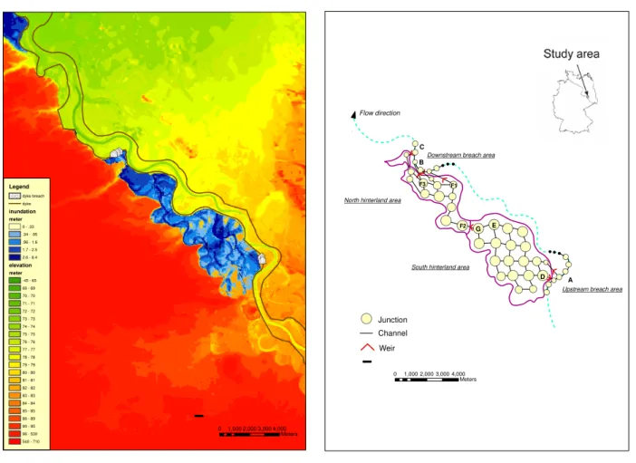
Fig. 2.The study area and the inundation hinterland(a)and the discretisation with junctions and channels of the studied hinterland(b).

3 Study site and model setup

The study site is the middle course of the Elbe River in Germany between the gages at Torgau (Elbe-km 154.2) and Lutherstadt Wittenberg (Elbe-km 214.1). This stretch of the river is heavily modified with dykes running along both sides for most of the flow distance. Characteristics of the discharges recorded at the gages at Torgau and Lutherstadt Wittenberg are given in Table 1. Dyke breaching only be-tween Elbe-km 154.2 and Elbe-km 192 was considered for the modeling exercise. There are no major tributaries flow-ing into the Elbe in this reach. High water level readflow-ings and the water level readings from the gage at Mauken (at Elbe-km 184.5) were used to compare measurements with hydrodynamic simulations. Model calibration and validation was carried out in another study (Lindenschmidt and Huang, 20072_{) with data from flood events in which breaching did}

not occur. Data from the Torgau gage during the most severe flood recorded (August 2002) was used as a boundary

con-2_{Lindenschmidt, K.-E. and Huang, S.: Simulating sediment and}

micro-pollutant transport in polder systems using a quasi-2D flood model, in preparation, 2007.

dition. The information on dyke breaches and the inundation area was drawn from the results of the 1D/2D simulation in this area (Vorogushyn et al., 2007). This model consists of a 1D hydrodynamic (St. Venant equation) model for the Elbe River, a dyke breach model to predict dyke breaching and a 2D storage-cell model for the simulation of inundation be-hind the dyke in the hinterland. The dyke breach model simu-lated the breach locations due to overtopping based on the ap-proach of Apel et al. (2004). From the results of this model, the dykes around Elbe-km 158 (upstream breach area) and between Elbe-km 173 and 179 (downstream breach area) are prone to breaching and the inundation area is shown in Fig. 2a. This model was used for comparison with simula-tions in this study and to test the performance of the quasi-2D modeling approach.

3.1 Input data

The discretisation of channels and junctions with inlet and outlet weirs is shown for the river and inundated hinterland in Fig. 2b. There are three pairs of weirs set for the simula-tion of breaches. Each pair constituents an inlet and an outlet for water flow. The inlet weir controls the water flowing into the hinterland and the outlet weir is used to simulate the back water after the flood peak in the river has passed and water flows from the hinterland back into the river. The first pair of weirs, which are near the river section A shown in Fig. 2b, represent the breaches on the upstream portion of the reach around Elbe-km 158 on the fourth day of the simulation. The breaches on the downstream portion of the studied reach (be-tween Elbe-km 173 and 179) were simulated by another two pairs of weirs near the river channel B and C, which eroded on the first and third simulation days, respectively. There is another weir set between the two parts of the hinterland to compensate for the difference in the average elevation of the hinterland land surfaces between these two parts (an average of 77.5 m and 79.5 m was calculated from a 50 m resolution digital elevation model for the northern and southern parts, respectively).

The simulation results are output on an hourly time step. A longitudinal profile of the maximum water level attained during the flood and the water level hydrograph recorded at Mauken (Elbe-km 184.5) were available for testing of the hydrodynamic model.

3.3 Local sensitivity analysis

Prior to the Monte-Carlo analysis, a sensitivity analysis was carried out to check the response of the system by varying different parameters. The parameters include:

1. Weir coefficient α from the weir discharge equation. The percentage deviations inαmay also represent the percentage deviation in weir breadthb, since both are multiplicative values in the weir equation. Onlyαwas used in the MOCA due to the linear compensatory ef-fect ofαandbon output variables (e.g. a 10% increase inαcan be compensated by a 10% decrease inb). 2. Roughness coefficientnof the channel bed from

Man-ning’s equation

3. Percentage deviations in the discharge boundary condi-tionqat the Torgau gage

The elasticityεwas used to quantify the local sensitivity of the input parameters:

ε= ∂O ∂P ·

P

O (5)

the resultOx. The elasticity then becomes: ε≈ 1O

1P · P O =

(Ox−Obase)

(Px−Pbase)

· Pbase

Obase

(6) SincePx=(1+x)·Pbasethe equation reduces to:

ε= 1 x

_O

x−Obase

Obase

(7) An elasticity value is calculated for each parameter used, which were increased by 10% separately for each single run. Hence,xequals 0.1 and the equation reduces to:

ε=₁₀·

_O

x−Obase

Obase

(8) 3.4 Global sensitivity analysis

Global sensitivity analysis apportions the output uncertainty to the uncertainty in the input factors, described typically by probability distribution functions that cover the factors’ range of existence (Saltelli et al., 2000). Here, the results from a Monte Carlo Analysis of 1000 model runs were an-alyzed to see the co-relationship among those variables and their contributions to the result. For the MOCA, the model-ing system was run 1000 times for which a new set of val-ues for the parameters were generated randomly from nor-mal probability distributions for each simulation run. A final MOCA was carried out in which all of the parameters were varied together to see the total effects on the output distribu-tion after 1000 simuladistribu-tions.

The parameters α, n and q were incremented or decre-mented within a±_{10% deviation range. Then values were} selected from normal distributions with ranges 1.17 to 1.43 for α, 0.034 to 0.042 forn (variation of roughness coeffi-cients in hinterland calculated for different land-use types, see Vorogushyn et al., 2007) and−0.1 to 0.1 forq (typical error range for discharge measurements, see Herschy, 1995; Lindenschmidt et al., 2005). Figure 3 shows the hydrograph used at the boundary condition at Torgau. The box-whisker plots illustrate the ±_{10% deviations used in the discharge} values for the MOCA. Note that the range of deviations in-creases with larger discharges.

To better interpret the behavior of uncertainty propagation through the modeling process and the contribution of the er-ror of each input value to the overall uncertainty in the model predictive outcome, the coefficient of variationCVwas used to standardize the input and output normal distributions for comparison of the MOCA results:

CV = Standard deviation

-1000 -2000 -3000 -4000 -5000

boundary

d

ischarge

(m

3/s

)

Q_1 Q_2 Q_3 Q_4 Q_5 Q_6 Q_7 Q_8 Q_9 Q_10

simulation day

10 1 2 3 4 5 6 7 8 9

Fig. 3. Hydrograph of boundary condition at Torgau with box-whisker plots indicating the range in the discharge deviation, which depict the minimum, maximum, medium and lower and upper quar-tiles of each sample group.

Fig. 4.Longitudinal profile of simulation day 5.2 and the high water marks, indicating the maximum water level attained.

4 Results and discussion

4.1 Hydrograph simulations

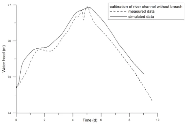
The first step in the model adaptation was to model the actual conditions of the August 2002 flood. A longitudinal profile of measured maximum water levels attained during this flood event was available for comparison of the hydrodynamic model results. Figure 4 shows good agreement between the simulated profiles at a simulation time of 5.2 days. The Man-ning’s roughness coefficient between 0.030 to 0.040 s/m1/3 provided the best fit of the simulations to the data. This value is somewhat higher than the one of 0.025 s/m1/3calibrated for the 1D/2D simulation by Vorogushyn et al. (2007). The water levels recorded at the gage at Mauken provided tempo-ral data for a comparison between measurements and

simula-Fig. 5.Measured and simulated water levels at the gage Mauken.

Fig. 6. Water levels in the river and hinterland. See Fig. 2b for locations A to G.

tion results which shows a good fit in Fig. 5. The simulations are somewhat overestimated, because the diversion of water due to dyke breaching is not included.

4.2 Dyke breach

Fig. 7.Comparison of water balances for upstream and downstream dyke breaches between the 1D/2D modelling and quasi-2D mod-elling.

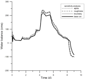
Fig. 8.The total water balance in the hinterland when each parame-ter was increased by 10% for the entire reach with breaching dykes.

and it is found that the water can only reach G after breach-ing in 36 h and F2 in 48 h. Hence it is obvious that the wa-ter travels faswa-ter in the quasi-2D model which may be due to the lower roughness values used for the hinterland sur-faces and the averaging of the terrain elevations in the two hinterland areas. To compare the result, the water balances between the upstream and downstream breaches, which indi-cate how much water is flowing through the breaches into the hinterland, were calculated for each modeling approach (see Fig. 7). The flow through the most upstream breach on Day 4 seems very abrupt for the 1D/2D model. Erosion of the dyke

Fig. 9. Water flowing through the upstream breaches at Elbe-km 158 when each parameter is increased by 10%.

Fig. 10. Elasticity analysis for the river channel; parameter sensi-tivity on water level.

for the 1D/2D model is an instantaneous process, whereas dyke erosion is allowed for in the quasi-2D model by suc-cessively lowering the weir crest over a six hour time frame. The flow behavior was similar for both modeling systems for the two most downstream dyke breaches during Day 1 and 3. The last breach occurred on Day 4 in the upstream breach area which leads to much more water flowing into the upper hinterland. The quasi-2D model simulated the back flow of water from the hinterland to the river more rapidly and ear-lier, which may also explain the rapid water flow through the hinterland.

4.3 Local sensitivity analysis

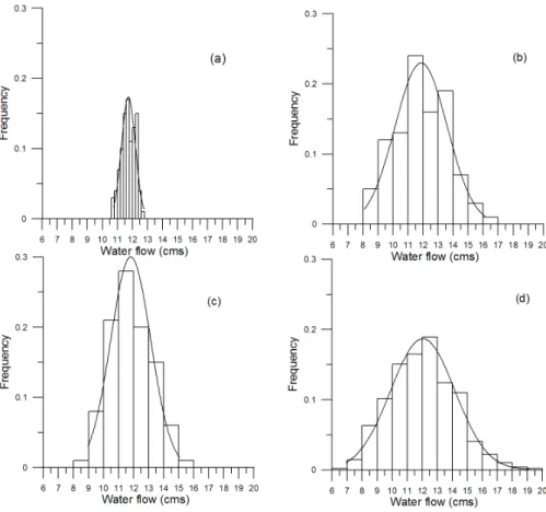
Fig. 11. Probability distribution of mean water flow during the first breach at F1 by varying alpha(a), roughness(b), boundary condition deviation(c)and all of these three parameters(d).

The sensitivity of the three parameters on water flow through the dyke breaches is similar as on the water balance (see Fig. 9). For the upstream breach area, the most sensitive parameter is the deviation in the boundary conditions, next is roughness, and least important isα. These effects are also re-flected in the elasticity analysis of each parameter on flow in the hinterland areas (data not shown). In this case, the elas-ticity remains fairly constant equaling about 1, which means a 10% increase of a parameter leads to a 10% increase in the result. It is also noticed that on the onset of water flow into or out of the hinterland, the elasticity on flow of each param-eter varies greater than during other periods, and the outflow is much more sensitive to parameter change than the inflow because the hinterland fills faster and the water flows back to the river earlier.

In addition, the water head along the whole river channel was analyzed. The major parameters influencing the head are the roughness and boundary condition deviations, because the water volume in the hinterland is not significantly large compared to the river flow (see Fig. 10, which shows the elas-ticity along the river when all of the dyke breaches occurred).

4.4 Global sensitivity analysis

In this study, all the parametersα,nandq were used together in the Monte-Carlo analyses. Figure 11 shows the probability distributions of water flow at F1 (refer to Fig. 2b) by varying each parameter separately or all three together. The mean value of these distributions does not differ much, ranging from 11.8 to 12.0 cms. However, the three variables together can lead to a wider range in the distribution. Both roughness and the deviations in boundary conditions contribute more uncertainty (broader distribution) to the result than does the weir coefficient.

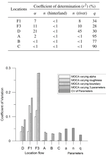
Figure 12 gives the CVs for each breach and the adjacent river channels. At all locations, there is an increasing trend in the CVs when all parameters are implemented in the MOCA. This is due to the increase in the number of varying param-eters in the model which leads to an increased spread in the distributions of the simulated results.αinfluences the results the least in both hinterland and river channels. The boundary condition is the main factor affecting the water flow through the river-hinterland system in the main channel. Bothnand

Locations Coefficient of determination (r )(%)

α n (hinterland) n (river) q

F1 7 <1 8 34

F3 11 <1 10 28

D 21 <1 45 30

A 2 <1 <1 95 B <1 <1 <1 77 C <1 <1 <1 90

Fig. 12. Coefficient of variations for four different Monte Carlo analyses by varying: i) alpha only; ii) roughness only; iii) boundary condition only and iv) varying all three factors simultaneously.

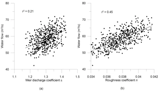
The co-relationship between the parameters and resulting variables can be explored using plots of scattered dots with the parameter values plotted in the x-axis against the vari-able values on the y-axis (see examples in Fig. 13). All the MOCA runs were used in whichα,nandqwere varied. The slope of the line indicates how the parameter values correlate with their respective variable results. Figure 13a shows the scatter plots of the parameterαplotted with the correspond-ing value of water flow at location D. A linear regression was plotted from which the coefficient of determinationr2 was calculated. For the water flow in the southern hinter-land area in the vicinity of the dyke breach, 21%, 45% and 30% (the latter not shown) of the total variation of the wa-ter flow values can be accounted for by a linear relationship with values ofα,n, andq, respectively. Table 2 summarizes the total variation on water flow at different locations in the river-hinterland system. Only the roughness coefficient in the river correlates significantly with water flows. The roughness

volumes in river channels and the effects of weir discharge and bottom roughness are stronger in the hinterland, espe-cially at the location D during the third breach. This is due to the high water level in the main channel at Day 4, so that

h in the weir equation is very large.

5 Conclusion and outlook

Several conclusions can be drawn from this study:

1. The quasi-2D approach is applicable in capturing the flood dynamics of a river reach in which dyke breach-ing has occurred. The 2D representation allows future modeling studies of sediment transport to quantify sedi-mentation and re-suspension during filling and draining of the hinterland.

2. The water balance at breach locations from the quasi-2D modeling results compared well with those obtained from the 1D/2D model from Vorogushyn et al. (2007). Flood water travels faster in the quasi-2D model due to the lower values used for bottom roughness in the hin-terland and due to the averaging of the hinhin-terland sur-face elevations.

3. The uncertainty in the bottom roughness and the bound-ary conditions contribute more significantly to the un-certainty of flow characteristics throughout the river-hinterland system than the parameters controlling dis-charge through the dyke breach.

Further study based on this modeling exercise will focus on the uncertainty analysis of the parameters, but with dif-ferent tools, such as SIMLAB, which is also designed for Monte-Carlo analysis. The water quality model TOXI will be added to simulate the transport and fate of sediments and heavy metals in the inundated areas. Furthermore, the pold-ers in the river system will also be included to see the influ-ence of dyke breaches and the polder control for peak dis-charge capping. Finally, this modeling section will be ex-tended to the gage at Wittenberg to check the effects of hy-drograph capping by dyke breaches and polder control on a larger scale.

Fig. 13.Co-relationship between the river water flow at location D (y-axis) and(a)α,(b)nin the adjacent river reach.

References

Ambrose, R. B., Wool, T. A., and Martin, J. L.: The Water Qual-ity Simulation Program, WASP5: model theory, user’s manual, and programmer’s guide, U.S. Environmental Protection Agency, Athens, GA, http://www.epa.gov/ceampubl/swater/wasp/, 1993. Apel, H., Thieken, A., Merz, B., and Bl¨oschl, G.: Flood risk

assess-ment and associated uncertainty, Nat. Hazards Earth Syst. Sci., 4, 295–308, 2004,

http://www.nat-hazards-earth-syst-sci.net/4/295/2004/.

Aureli, A., Maranzoni, A., Mignosa, P., and Ziveri, C.: Flood haz-ard mapping by means of filly-2D and quasi-2D numerical mod-eling: a case study, in: Floods, from defence to management, edited by: van Alphen, J., van Beek, E., and Taal, M., 3rd Iinter-national Symposium on Flood Defence, Nijmegen, Netherlands, Taylor & Francis/Balkema, ISBN 0415391199. Blain, pp. 373– 382, 2006.

Bates, P. D. and De Roo, A. P. J.: A simple raster-based model for flood inumdation simulation, J. Hydrol., 236(1–2), 54–77, 2000. Chua, L., Merting, F., and Holz, K. P.: River inundation mod-elling for risk analysis, 1st International Conference on River Basin Management, edited by: Falconer, R. A. and Blain, W. R., pp. 373–382, 2001.

D’alpaos, L., Defina, A., and Mattichio, B.: 2D finite element mod-eling of flooding due to river bank collapse, Proc. Modmod-eling of Flood Propagation Over Initially Dry Areas, American Society of Civil Engineers (ASCE), edited by: Molinaro, P. and Natale, L., 60–71, 1994.

Han, K. Y., Lee, J. T., and Park, J. H.: Flood inundation analysis resulting from levee break, Journal of Hydraulic Research, In-ternational Association for Hydraulic Research (IAHR), 36(5), 747–759, 1998.

Herschy, R. W.: Streamflow measurement, 2nd edition, E & FN Spon, an imprint of Chapman & Hall, UK, 1995.

Huang, S., Rauberg, J., Apel, H., and Lindenschmidt, K.-E.: The effectiveness of polder systems on peak discharge capping of floods along the middle reaches of the Elbe River in Germany, Hydrol. Earth Syst. Sci. Discuss., 4, 211–241, 2007,

http://www.hydrol-earth-syst-sci-discuss.net/4/211/2007/. Lindenschmidt, K.-E., Rauberg, J., and Hesser, F.: Extending

un-certainty analysis of a hydrodynamic – water quality modeling system using High Level Architecture (HLA), Water Quality Re-search Journal of Canada, 40(1), 59–70, 2005.

Lindenschmidt, K.-E., Rauberg, J., and Hohmann, R.: Stofftrans-port im Fluss- und Auenbereich bei Hochwasser: Quasi-2D hy-drodynamische Simulation und Unsicherheitsanalyse, Gas- und Wasserfach: Wasser und Abwasser, 147(11), 720–729, 2006. Saltelli, A., Chan, K., and Scott, E. M.: Sensitivity analysis, John

Wiley & Sons, Ltd., pp. 10, 2000.