The impact of social security reform on occupational and retirement behavior : a quantitative assessment for Brazil

(1)

FUNDAC

¸ ˜

AO GETULIO VARGAS

ESCOLA DE P ´

OS-GRADUAC

¸ ˜

AO EM

ECONOMIA

Rafael Machado Parente

The Impact of Social Security Reform on Occupational

and Retirement Behavior: A Quantitative Assessment for

Brazil

(2)

Rafael Machado Parente

The Impact of Social Security Reform on Occupational

and Retirement Behavior: A Quantitative Assessment for

Brazil

Disserta¸cão submetida a Escola de P´ os-Gradua¸cão em Economia como requisito parcial para a obten¸cãoo do grau de Mestre em Econo-mia.

Orientador: Pedro Cavalcanti Gomes Ferreira

(3)

Ficha catalográfica elaborada pela Biblioteca Mario Henrique Simonsen/FGV

Parente, Rafael Machado

The impact of social security reform on occupational and retirement behavior: a quantitative assessment for Brazil / Rafael Machado Parente. – 2016.

39 f.

Dissertação (mestrado) - Fundação Getulio Vargas, Escola de Pós-Graduação em Economia.

Orientador: Pedro Cavalcanti Gomes Ferreira. Inclui bibliografia.

(4)

(5)

Agradecimentos

Agrade¸co aos meus pais, Pedro e Lúcia, que tanto me ajudaram ao longo deste caminho. Em particular, por sempre ressaltarem o cunho social da economia, assim como a importância da didática, que muitas vezes são esquecidos durante o processo. Meu irmão, André, por todas as reflexões induzidas por conversas despretensiosas ao fim do dia, e pelo apoio e companhia fundamentais para que este objetivo pudesse ser realizado.

Agrade¸co à Ana Luiza Dutra por prover condi¸cões necessárias e suficientes para o meu, até então, sucesso acadêmico. Presente durante todo o trajeto, me amou, acalmou, orientou, apoiou e ajudou, de forma a exaurir qualquer conjunto de palavras que existiriam para agradecer completamente a ela.

Ao meu orientador, Pedro Cavalcanti, pela paciência ao longo do desenvolvimento desta disserta¸cão, pelo tempo utilizado em discussões frut´ıferas e apoio e ajuda constantes ao longo do segundo ano do mestrado. A Cézar Santos e Fernando de Holanda Filho, agrade¸co os comentários fornecidos, que ajudarão no desenvolvi-mento deste projeto.

`

A minha turma na EPGE, sem a qual eu n˜ao seria metade do economista que hoje sou.

(6)

Abstract

Population ageing is a problem that countries will have to cope with within a few years. How would changes in the social security system affect individual behaviour? We develop a multi-sectoral life-cycle model with both retirement and occupational choices to evaluate what are the macroeconomic impacts of social security reforms. We calibrate the model to match 2011 Brazilian economy and perform a counterfactual exercise of the long-run impacts of a recently adopted reform. In 2013, the Brazilian government approximated the two segregated social security schemes, imposing a ceiling on public pensions. In the benchmark equilibrium, our modelling economy is able to reproduce the early retirement claiming, the agents’ stationary distribution among sectors, as well as the social security deficit and the public job application decision. In the counterfactual exercise, we find a significant reduction of 55% in the social security deficit, an increase of 1.94% in capital-to-output ratio, with both capital-to-output and capital growing, a delay in retirement claims of public workers and a modification in the structure of agents applying to the public sector job.

(7)

List of Figures

1 Life Expectancy . . . 17

2 Calibrated Survival Probabilities and Population Age Profile. . . 25

3 Cost Function. . . 26

4 Efficiency Age Profile . . . 28

5 Agents’ Equilibrium Distribution in the Steady State. . . 30

6 Economic Participation Rate. . . 31

7 Public Test Takers. . . 32

8 Average Savings and Consumption. . . 33

9 Average Savings. . . 34

10 Test Takers. . . 34

11 Agents’ Distribution. . . 35

(9)

List of Tables

1 The Social Security Factor . . . 18

2 Log of income per hour. Source: 2011 PNAD . . . 27

3 External Calibration Summary . . . 29

4 Internal Calibration Results . . . 29

5 Distribution of Individuals (%) . . . 30

6 Participation Rate (%) . . . 30

(10)

1 Introduction

This work will explore quantitatively the effect of modifications in the social security system on occupational and retirement behavior. The importance of this subject relies on future problems that several countries should face due to both their ageing population and the financial fragility of their current social security scheme. In particular, we will analyse what impacts segregated1 social security systems, and potential reforms, have on individual and aggregate behavior.

Population ageing is the result of increasing life expectancy and falling fertility rates. Ac-cording to the UN, world’s life expectancy has been increasing steadily in the last 15 years. In 2000, life expectancy at birth was 65 years old. Nowadays, an individual is expected to live 70.5 years. Dependency ratio2 _{is expected to increase from 13% nowadays to 26% in 2050 and 38%} in 2100. Bl¨ondal and Scarpetta (1999) and Gruber and Wise (2002) provided evidence that the workforce participation of the elderly population has declined in many COED countries.

Pay-as-you-go (PAYG) social security systems exist in most of the countries in the world. Some of them have differentiated pension rules for public servants. According to the World Bank, most public schemes are not financially sustainable, even if we do not consider the demo-graphic transition problem. The sustainability problem enhances the government’s budgetary deficit, inducing negative macroeconomic consequences. An important example is the crisis that occurred in Brazil in the aftermath of the East Asian and Russian financial meltdowns, in 1998. It was documented that a fiscal deficit of more than 6% of the GDP triggered this crisis, and that two thirds of this deficit was due to the cost of pensions. In Lebanon, public retirees’ pensions is the third greatest expenditure item in the government’s budget, even though they account for approximately 3% of the population.

As it is well known from the literature, PAYG systems tend to distort consumption, labor and asset accumulation decisions. Whether this distortion generates or not welfare gains is an important issue, once the ageing population tend to pressure the necessity for more benefits which, in any reasonable economic environment, should be financed at some cost. Facing this, should the government maintain the contribution rates of the workers and diminish the value paid as social security benefits, should it raise labor taxes to finance an increasing value of benefits given to the newly retired agents or should they simply cut other social expenditures, such as expenditures in health and education?

Brazilian demography prospects follow global trends. The average number of births per woman has been decreasing steadily since 1980. At the same time, life expectancy raised substantially. According to the World Bank, Brazil’s life expectancy has raised from 54.69 years in 1960 to 73.62 in 2012. According to Brazilian Institute of Geography and Statistics’ (henceforth IBGE) projections, the share of individuals aged 65 and over is projected to jump from 4% in 1980 to 22% around 2050. As a combination of these facts, the dependency rate will likely follow a U shape in the years ahead, so that it is important to use the demographic bonus to generate the wealth that will be used to finance the higher expenditure to support the elderly population in the future.

The Brazilian’s pension system ranks among the most generous in the world. Tafner et al. (2015) regress social security expenses3_{and the dependency ratio in a sample of 35 countries, in} 2009. Brazil’s dependency ratio was around 10.1, and its social security expenses was 10.8% of GDP. For the dependency ratio observed, the regression predicts that Brazilian’s social security expenses should be around 3.8% of the GDP. On the other hand, given the SS expenses, the regression predicts a much older country, with a dependency ratio around 29. The reason for this problems lay, essentially, in the Brazilian’s social security structure.

The constitutionally guaranteed provision of the so called “integrality” ensured that public

1_{Different rules for public and private retirees.}

2_{The ratio of individuals that have more than 65 years old and that are aged between 15 and 64.}

(11)

sector pensions would match the average of the 80% highest salaries before the retirement date. On the other hand private benefits are defined as the arithmetic average of the 80% higher salaries over the life-cycle up to an upper limit, which does not reach 10 times the minimum wage. Therefore, the retirement benefit for private workers is potentially much lower than that of public workers.

Early retirement among both public and private workers is also a serious problem the Brazil-ian government will face in the next few years. This is essentially because the retirement age is still relatively low in Brazil, once the country does not have a minimum retirement age for those in the private sector who have contributed to the social security system for 35 years or more. According to Rocha (2007), the average age in which men ask for retirement under length of contribution (LC) modality is 56, whereas the world’s average is 62, the OECD’s average is 64 and the Latin America’s 62.

The main goal of this project is to quantitatively assess questions such as: (i) how segregated social security systems (and potential reforms) affect individual decisions? (ii) what types of agents would be more affected by a potential change in the structure of retirement in Brazil? and (iii) how reforms that already happened in the Brazilian economy ameliorated (or not) the social security system’s problems?

To access such future questions, we developed a multi-sectoral life-cycle model and cali-brated it to match key aspects of the 2011 Brazilian economy. Our calicali-brated model reproduces Brazilian features regarding sectoral and labor decisions, retirement claims characteristics, as well as social security deficit and the public job application decision. Other aspects, such as the shape of average consumption and savings curves are also in line with the literature on life-cycle economies.

In particular, we evaluate the long-term macroeconomic effects of the 2013 social security reforms. These reforms ended the “integrality” provision for public retirees, imposing a cap on public benefits and approximating both social security regimes. The main impacts were the following: (i) a reduction of 55% in the social security deficit; (ii) an increase of 1.94% in capital-to-output ratio; (iii) an increase in average savings, mainly induced by public sector workers who now face worse retirement conditions; (iv) a delay in the retirement claims of the public workers and a modification in the structure of the agents applying to the public sector job and (v) the shift of unproductive workers towards the private sector, once the retirement sector has lost part of its attractiveness. On top of that, we perform a long-run welfare analysis which indicates that individuals are 3.3% better off, in terms of consumption equivalence, relatively to the old steady state equilibrium.

The rest of the paper proceeds as follows. Section 2 relates our work with the literature of life-cycle models with heterogeneous agents, retirement aspects and multi-sectoral economies. Section 3 presents the key features of our model, including the problem of the agents and the stationary distribution. Section 4 defines the equilibrium concept we used in this work. Section 5 describes the calibration procedure. Section 6 validates our numerical solution, comparing non-targeted moments that our model generates to the data. In Section 7, we briefly detail the 2013’s social security reform, perform the counterfactual exercise and analyse the steady state implications it. Section 8 accesses the long-run welfare impacts of the recently adopted reforms. Finally, Section 9 concludes the work, summarizing our main findings.

2 Related Literature

(12)

accounted for little less than half of the wealth held by the top 1%. However, the social security structure modelled in Huggett (1996) was very simple, with exogenous retirement decision and fixed benefits over all agents.

Following the approach used in Huggett (1996), Huggett and Ventura (1999) and Conesa and Krueger (1999) both studied potential social security reforms and their macroeconomic impacts. They introduced a more complex social security structure, allowing the benefits to be functions of the average past earnings.

Huggett and Ventura (1999) analysed how modifications in the social security system would affect the distribution of consumption, welfare and leisure. Their main findings do not support the implementation of an alternative social security system. In particular, they analyse a two-tier system, the first being a mandatory, defined-contribution pension scheme and the second a scheme that guarantees a minimum retirement income. A key problem in their analysis is that they compared steady state equilibria, whereas the transition analysis is equally important, once the government should account for political support to realize such major reforms.

Conesa and Krueger (1999) stress out how a PAYG social security system is considered by the agents as a partial insurance device against idiosyncratic risks over the life-cycle. They analyse the transition path of potential reforms on the social security scheme. Their main finding is that any reform would not gain majority support, if we were in a political competition model. Another interesting question that they discuss is how one can reverse the majority support of a reform by analysing a partial equilibrium model, and how important are the general equilibrium effects in determining welfare consequences.

More recently, Belush and Bohacek (2009) built a life-cycle general equilibrium model with endogenous fertility to better understand the macroeconomic impacts of a social security reform when agents face fertility decisions. They found that models with exogenous fertility usually underestimate the equilibrium aggregate capital stock. Highly educated workers save more in financial assets than in terms of children, therefore a steady state in which agents choose how many children they would have tend to have a higher aggregate capital stock than in a otherwise similar steady state equilibrium with exogenous fertility.

The aforementioned papers treat retirement exogenously. When an individual reaches a certain age, he starts collecting his benefits as a retiree. This is not a plausible assumption to address early retirement provisions, for instance, a common problem in Brazil. Even though agents can enhance their future benefits by going to work, there is no tradeoff between staying one year longer as a worker to raise his future benefits and asking for retirement one year sooner to collect the benefits for a longer period. Imrohoroglu and Kitao (2012), Ferreira and dos Santos (2013) and Jung and Tran (2012) are, among others, papers that started treating retirement application endogenously.

Jung and Tran (2012) analyse what are the impacts of an extension in the social security coverage over the elderly workers in the informal sector. The way in which they model infor-mality is closely related to the one used in the present paper. The welfare analysis they made suggests that the insurance effect overcompensates the distortion effect that a bigger social security scheme has on individual behavior.

Imrohoroglu and Kitao (2012) study the impact of two social security reforms on the US economy. They introduced health heterogeneity, as well as medical expenditures, which could act as determinants of social security benefit claims decision. By raising the early retirement age in two years, the authors could not find any significant effect in such experiment. On the other hand, by raising the normal retirement age in two years, they found significant increases in the aggregate capital stock and labor supply. A key issue in their work is that they compare steady states, whereas a lot of what is going on in terms of welfare could be in the agents that were actively working when the reform was implemented, hence can retire themselves under the old rules.

(13)

agents between 1950 and 2000 shows that most of the changes in the retirement profile are due to the changes in the social security scheme and the introduction of the Medicare program.

None of the papers so far addressed retirement choices when agents faces more than one working sector. Segregated social security systems and the case of Brazil are dealt in Glomm et al. (2009), dos Santos and Pereira (2010), Dos Reis and Zilberman (2014) and Cavalcanti and dos Santos (2011).

Glomm et al. (2009) develop a life-cycle economy to analyse the implications of early re-tirement in aggregate variables. The authors assess the efficiency gains from eliminating an overpaid public retirement system. They abstract from individual uncertainty and from en-dogenous migration decision between the public and private sector, and analyse the policy reform implemented in 2003. In this paper, differently from Glomm et al. (2009), we will deal with sectoral choice and allow for idiosyncratic productivity.

Cavalcanti and dos Santos (2011) study how an overpaid public sector, as the one in Brazil, could cause the misallocation of resources. The best human capital in the economy can end up in a sector that is not very productive, but very attractive in terms of insurance against income fluctuations. Dos Reis and Zilberman (2014) stress the insurance role of the government sector in the Brazilian economy. They study how agents would tend to use this sector as an insurance device against income fluctuation and idiosyncratic shocks. dos Santos and Pereira (2010) develop a life-cycle model to determine what are the macroeconomic consequences of different tax reforms.

What the literature have not done yet is to develop a model to study occupational and retirement choices of agents that face a bi-sectoral retirement structure, as in Brazil. As an application of our model, we quantify the macroeconomic effects of the 2013 reform of the social security scheme, which imposed a ceiling on public pensions, approximating retirement in public and private sectors.

3 The Model

The economic environment in this paper consists of a life-cycle model of occupational choice and retirement behavior. Individuals can be either in the private sector, working for the government or retired from the labor force. All decisions are endogenous, in the sense that the individual will only ask for retirement or apply to the public sector job if it is worth it.

Aggregately, we have a two-sector economy with public and private production. Since the main purpose of this project is to see how individuals respond to modifications in the social security system, the government sector in the present environment is modelled in a simple manner. The government sector is responsible for paying non-competitive wages to its workers (in exchange for the production of a fixed amount of a public good) and for managing a PAYG retirement pension system for both public and private sectors. In order to pay its bills, the government taxes consumption, capital and labor income.

The sources of exogenous uncertainty in the economy come from idiosyncratic shocks the private workers have in their labor efficiency, the life span of the agents and the probability of migrating to the informal sector, as will be described below.

3.1 Demography, Preferences and Choices

(14)

The age profile of the population, denoted by {ϕt}Tt=1 is modelled by assuming that the fraction of agents at agetin the population is given by the following law of motionϕt= ₁₊ψ_gt_nϕt−1

and satisfies T

P

t=1

ϕt= 1, where gn denotes the population growth rate4.

Agents enjoy utility over consumption,ct, leisure,lt, and a public good YG. They maximize their expected utility throughout life:

E0 " _T

X

t=1

βt−1

t

Y

k=1

ψk

!

u(ct, lt, YG)

#

Whereβ is the intertemporal discount factor andEtis the expectation operator conditional on timet. The agents’ period utility is assumed to take the form:

u(ct, lt, YG) =

[(ct+ǫYG)γ(1 +lt)1−γ]1−σ 1−σ

Whereσ determines the risk aversion parameter and γ denotes the share of consumption in the utility. Besides private consumptionct, the household’s utility is also influenced by a public good, YG (if ǫ6= 0). If ǫ <0, the marginal utility of consumption increases with an increase in

YG and if ǫ > 0, the opposite is true. Thus, our framework also allows for substitutability or complementarity between public and private goods.

In this economy, each agent can be: (i) a private worker (either formal (P F) or informal (P I)); (ii) a public servant (G); (iii) a private retiree (either by age modality (RPage) or length of contribution modality(RP)) and (iv) a public retiree (also either by age modality (RGage_{) or length of contribution modality (}_RG_{)). We will denote this individual state as}

m∈ {P F, P I, G, RP, RPage_{, RG, RG}age_}5_.

What are the decision variables for each type of agent? First of all, agents choose how much to consume, ct ≥0. They also make a labor decision, Lt. We will restrict the labor choice to be in {0,1}. The remaining time is considered to be entirely leisure time. We assume that all retirees are in the formal private sector and that public servants are obligated to go to work. We further suppose that retirees cannot reenter the public sector.

Agents can choose to take the open exam and try their luck into the public sector. Taking this exam is costly, where the time cost of it is a function of their current age, cap(t). Since retirees cannot enter the public sector, they will never opt for paying the cost and taking the public exam. Public workers cannot retake the exam, by assumption.

As the workers become older, and conditional on meeting the eligibility requirements, they can apply for social security benefits and become retirees within their respective sector next period. It is worth to notice that the informal private workers retire as private retirees, the same retirement sector as the formal private workers (there is no informal retirement sector).

All agents in the economy can save and lend their savings to a private competitive firm, as usual.

We further assume that both the public and retirement sectors are absorbing states. Once a worker applies and enters the public sector, there is no turning back. The same is true for the application for social security benefits.

3.2 Labor, Income and Efficiency

Conditional on the sectoral choice, the individuals make decisions on whether to work or not and asset accumulation. Let wdenote the competitive wage paid by the private firms to their

4_For

t= 1, it is easy to show thatϕ1=

1 + T

P

t=2

(1 +gn)−(t−1) t Q i=2 ψi −1 .

(15)

respective private workers. Thus, an individual agedtwho decides to workLt∈ {0,1−cap(t),1} produces a total of units of consumption before taxes given by6_:

yt(m) =

(

wezt+ηt_L

t if m∈ {P F, P I, RG, RP, RPage, RGage} (1 +θ)wezG _if _m₌_G

In the model,zt(the idiosyncratic productivity) is a random variable that evolves according to an AR(1) process given by: zt =λzzt−1+εz, with εz ∼N(0, σz2). There is no uncertainty regarding the public sector. zGis the productivity that the private worker had when he decided to take the admission test for the public sector and succeeded. In our model, it will be constant over time. ηt is a deterministic age-specific component, applied only to the private sector workers. The parameter θ corresponds to the wage premium or economic rent that public sector workers receive relative to their counterparts in the private sector and thus it accounts for the political component of wage determination in the public sector.

All agents in the economy pay capital income tax τk and consumption tax τc. Workers face labor income taxes (τy(m),τss(m)) , where the revenue from τss(m) is used to finance the social security benefit payments to the retirees, and the revenue from τy(m) finances overall government expenditures not related to the social security system. Retirees pay a tax rate of

τb(m) over their social security benefits. Agents in the private sector that are informal workers do not pay labor income taxes.

We assume that individuals save in a risk-free asset which pays an interestr. They cannot have negative assets at any age, so that the amount of assets carried over from age t to t+ 1 is such thatat+1 ≥0. Furthermore, given that there is no altruistic bequest motive and death is certain at age T + 1, agents at age T consume all their assets, that is, aT+1 = 0. We will normalize the continuation value after ageT as zero.

The budget constraint for the non-retired individuals in the private sector (m∈ {P F, P I}) is given by:

(1 +τc)ct+at+1 = [1 + (1−τk)r]at+ (1−τy(m))yt(m)−τss(m) min{yt(m), ymax}+ζt

The budget constraint for the public sector workers is:

(1 +τc)ct+at+1= [1 + (1−τk)r]at+ (1−τy(G)−τss(G))yt(G) +ζt

The budget constraint for the retirees (m∈ {RP, RG, RPage_{, RG}age_}_{) is:}

(1 +τc)ct+at+1 = [1 + (1−τk)r]at+ (1−τy(P F))yt(m) + (1−τb(m))b(·) +ζt

Where b(·) stands for the social security benefits that a retiree (either public or private) will receive. Further on we will describe what are the arguments of the social security benefits function.

3.3 Informal Sector

Individuals in the private sector can be formal or informal. The main difference is that in the latter case, agents do not pay labor income taxes and cannot enhance their length of contribution to the social security system or their average past earnings.

Informal employment is treated as a shock. In particular, at each period, formal private sector workers can migrate to informality tomorrow with probability 1−PF. With probability

PF, tomorrow they will remain working for the formal private sector.

It should be stressed that, while keeping the model tractable, this modelling strategy allows us not to rule out informality, which accounts to a significant share of private sector in Brazil.

6_{Note that it is already imposed that the public workers must work,}

(16)

In addition, note that being an informal worker is still a choice since private worker agents can always stay at home.

Given that workers in the informal sector have, on average, lower human capital, we allow

PF to depends on human capital as follows:

PF(zt) =

θF

θF +e−

(_zt−z˜)

σz

Where ˜z is the unconditional mean of the exogenous discrete process of zt.

It is worth noticing that the parameter θF influences directly the mass of the stationary private workers that will belong to the formal private sector.

3.4 Public Sector Recruitment

According to constitutional rules, the hiring process of civil servants is provided by public competition. Thus, agents in the private sector who want to work in the public sector must take open exams and only those who obtain the best grades on these tests become eligible to fill a pre-determined number of job positions.

Once a private worker takes the test and succeeds, he necessarily will become a public servant next period. There is no turning back in our model, in the sense that once you passed the exams, you must work for the government until retirement.

The timing of the model is the following. First, an agent chooses to apply at t, paying the time costcap(t). His score is revealed att+ 1: qt+1 ∼U[0,1]. Ifqt+1 ≥q¯the he will necessarily work for government att+ 1. Otherwise, he will remain a private worker. The threshold score, ¯

q, is chosen by the government in equilibrium to balance the demand and supply of public servants.

3.5 Social Security System

The social security in Brazil is a pay-as-you-go system, which transfers income from workers to retirees. The system is financed with payroll taxes, and has two very different regimes - the private sector regime and the public sector regime. The benchmark year of our calibration is 2011, hence the retirement benefits structure is modelled in order to mimic the retirement rules that used to prevail in Brazil at that year.

3.5.1 Private Benefits

The private sector regime is organized under INSS, which stands for Instituto Nacional do Seguro Social (National Institute of Social Security), and establishes a contribution rate according to wage levels. Under the INSS retirement sector, we have two modalities of retirement - the age modality and the length of contribution modality.

If the worker is older than the normal retirement age, which is 65 years old, and have contributed more than 15 years in the formal private sector, he can apply for retirement under age modality. If the worker is older than 65 years old and has a labor income,y, less or equal to

1

4ymin, whereymin is the minimum wage of the model economy, he can also apply for retirement. In this case, he will receiveymin as benefits, independently from his history of contributions. If the worker has not achieved the normal retirement age but have contributed more than 35 years to the social security system, he can ask for retirement under length of contribution modality. In both modalities, the value of the benefits will be calculated as a fraction of average past earnings,x:

b(tr, x, m, tC, y) =

(

max{Ψ(tr, m, tC)x, ymin} if (y≤ 1₄ymin &tr ≥65)

Ψ(tr, m, tC)x otherwise

(17)

20 30 40 50 60 70 80 90 0

10 20 30 40 50 60

Life Expectancy

Age

Figure 1: Life Expectancy

Where Ψ(t, m, tC) denotes the retirement replacement rate as a function of the age in which the worker asked for retirement, tr, the retirement modality, m, the number of years that the worker contributed formally to the social security system,tC, and the current labor income, y. The average lifetime earnings,x, is calculated by taking into account individual earnings up to the age of withdrawal from the labor force that are lower than the maximum taxable income,

ymax. Thus, the law of motion for x can be written as:

xt+1 =

xt(t−1) +min{yt(P F), ymax}

t , fort= 1,2, ..., t

r ₍₁₎

Note that only earnings from the formal sector are considered in the calculation of x. This is so because we assume that individuals in the informal sector are prohibited to contribute to the social security system.

For those who apply for benefits under the length of contribution modality, the replacement rate is given by:

Ψ(tr, RP, tC) =

(

f(tr_{, t}

C) for tC ≥35

−B¯ for tC <35

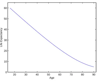
Where ¯B is a positive high-valued number7 and f(tr, tC) is commonly known as the “fator previdenci´ario” which is not necessarily between [0,1]. Such discount was implemented by the Fernando Henrique Cardoso’s presidency, in order to discourage the early retirement that occurred in Brazil, mainly before the year of 1999. Its formula is constitutionally given by:

f(tr, tC) = 0.31tc

E(tr₎

1 +(t

r_{+ 0}_.₃₁_t C) 100

Where E(t) is the life expectancy of the individual. Figure 1 plots how the 2011 life ex-pectancy, published by IBGE, looks like.

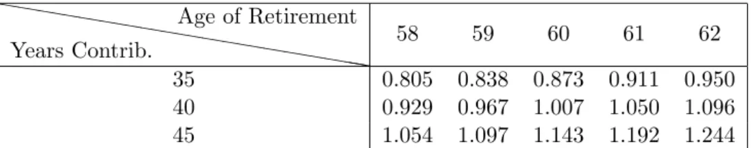
Depending on the number of years that the private worker has contributed to the social security system and on the age of retirement,f can be bigger than 1. From now on, we will call

f the social security factor. Table 1 gives us some idea of what values this factor has, depending on the age of retirement and the number of years of contribution to the formal sector.

(18)

Table 1: The Social Security Factor ❤❤❤ ❤❤ ❤❤ ❤❤ ❤❤ ❤❤ ❤❤ ❤❤ ❤❤ Years Contrib.

Age of Retirement

58 59 60 61 62

35 0.805 0.838 0.873 0.911 0.950

40 0.929 0.967 1.007 1.050 1.096

45 1.054 1.097 1.143 1.192 1.244

Under the age modality, since the worker has already waited until the normal retirement age to retire himself, the social security factorf is only applied if it enhances the benefits received - that is, iff is greater than one. Therefore, the replacement rate will be given by:

Ψ(tr, RPage, tC) =

(

max{f(tr, tC),1}Ψ(˜ tC) for tC ≥15

−B¯ for tC <15

Where ˜Ψ(tC) is an additional discount, in which individuals aged 65 and over who have met the fifteen years minimum contribution requirement are entitled to 85% of their adjusted lifetime earnings: max{f(t, tC),1}x. For each additional year worked beyond the lower limit, this fraction increases in one percentage point up to 100%. Such additional discount can be formally written as:

˜ Ψ(tC) =

(

0.70 + tC

100 for 15≤tC <30

1 if tP ≥30

3.5.2 Public Benefits

According to constitutional rules, the hiring process for civil servants is provided by public competition. Once approved, selected and hired, civil servants have special rights, including a different pension system. In particular, retirement benefits for civil servants do not have an upper limit and correspond to the average of the 80% highest wages received during the public career. Since we assume that there is no uncertainty regarding the labor income in the public sector, such average equals the last wage. Furthermore, retirement is mandatory at age 70 in the public sector and the individual must have at least 10 years of public sector working.

Civil servants older than 60 and that have contributed for at least 30 years can apply for benefits under the length of contribution modality. Using the same “ ¯B-trick” as before, the benefits given to the public servant can be expressed as:

b(zG, RG, tC, tG, y) =

(

(1 +θ)wezG _for_t

C ≥35 and tG≥10

−B¯ otherwise

Where tC is the number of years that the public worker contributed to the Social Security System, tG is the number of years that the individual has worked as a public servant and y is the current labor income.

Civil servants older than 65 can apply for benefits under the age modality. In this case, individuals are entitled to a proportion tC

35 of their last wage. It should be noticed that this formula entails low benefits for agents that reach 65 with a small number of contributions. If the public servant is older than 65 years old and has a labor income less or equal to 1₄ymin, he can also apply for retirement under age modality. As in the private retirement case, his benefits will be equal toymin, independently from his history of contributions. Formally, we have:

b(zG, RGage, tC, tG, y) =

          

min{tC

35,1}(1 +θ)wezG iftG≥10 and y > 14ymin max

min{tC

35,1}(1 +θ)wezG, ymin iftG≥10 and y≤ 14ymin

ymin iftG<10 and y≤ 1₄ymin

(19)

3.6 Value Functions

For a given age, we will divide the individual states depending on what sector of the economy the individual is located. The state of an agent in the private sector (both formal and informal) is sm = (a, z, x, tC) ∈ Sm ≡R+× Z × X × {0,1, ..., T}, for m∈ {P F, P I}, where a represent his asset holdings, z is the agent’s idiosyncratic productivity in the private sector, x is his average past earnings in the private sector and tC is the length of contribution the agent has in the formal sector. The relevant individual state for a public worker is sG = (a, z, tC, tG) ∈

SG ≡ R+× Z × {0,1, ..., T} × {1, ...,10}. As for the retirees, their relevant state is given by

sm = (a, z, b) ∈Sm ≡R+× Z × B, for m ∈ {RP, RG, RPage, RGage}, where b stands for the benefits that these retirees are receiving.

Now we turn ourselves to the recursive problem for each agent in our economy. By solving the below problems for all agents at all living periods, we will get the policy functions: (i) the optimal leisure decision dl,t : Sm → {0,1}, the public sector application decision dap,t : Sm → {0,1} the asset holdings decisions da,t : Sm → R+ and consumption policies dc,t : Sm → R++ for all m ∈ {P F, P I, G, RP, RG, RPage_{, RG}age_} _{and (ii) (}_dss

t , d ss,age

t ) : Sm → {0,1} retirement decisions form∈ {G, P F, P I}.

3.6.1 Retired Workers

Since retirement is an absorbing state, the value functions for those type of agents are quite simple. For m∈ {RP, RG, RPage_{, RG}age_}_{, the value function of a retiree is given by:}

Vt(sm) = max

(c,a′₎_≥₀_{, l}_∈{₀_,₁_}u(c, l, YG) +βψt+1·E

Vt+1(s′m)

s.t. (1 +τc)c+a′ = [1 + (1−τk)r]a+ (1−l)wezt+ηt+ (1−τb(m))b+ζ Wheres′_m = (a′, z′, b) andE[Vt+1(s′m)] =

P

z′

Π(z, z′)Vt+1(s′m) is the standard expected value conditional on the current productivity,z.

3.6.2 Public Servants

At each age t, the public sector worker is always choosing what is best for him among three options: (i) asking for retirement under Length of Contribution modality, if eligible; (ii) asking for retirement under Age modality, if eligible and (iii) not asking for retirement today and continue next period as a worker.

In case he decides to retire himself, the social security benefits that he will earn from tomorrow on are calculated according to the social security section above. Call them b′. Since we will solve the model numerically, there will be a grid space for the benefits of the retirees,B. Notice that b′ will not necessarily be onB, so we interpolate the retiree’s next period expected value function: _Eb[Vt+1(s′RG)] ≡ αb ·E

Vt+1(a′, z′, b1)+ (1−αb) ·E

Vt+1(a′, z′, b2), where

b1, b2 ∈ B are such that b′ =αbb1+ (1−αb)b2.

Let us start deriving the problem of an agent that is younger than 58. When t≤ 58, the worker is not eligible to any retirement modality. His value function is given by:

Vt(sG) =VtN R(sG)

WhereV_tN R(sG) is the value function of not asking for retirement:

V_tN R(sG) = max

(c,a′₎_≥₀u(c,0, YG) +βψt+1Vt+1(s

′

G)

(20)

Wheres′_G= (a′, z, tC+ 1, tG+ 1). Whent∈[59,63], a public servant can ask for retirement in the length of contribution modality. His value function will be the maximum between asking for retirement and keep working:

Vt(sG) = max{VtN R(sG), VtRG(sG)}

Being V_tN R(sG) the same as before and denoting VtRG(sG) as the value function of asking for retirement:

V_tRG(sG) = max

(c,a′₎_≥₀u(c,0, YG) +βψt+1Eb

Vt+1(s′RG)

s.t. (1 +τc)c+a′ = [1 + (1−τk)r]a+ (1−τss(G)−τy(G))(1 +θ)wezG+ζ

Where s′_RG = (a′, z′, b′ = b(zG, RG, tC + 1, tG+ 1,(1 +θ)wezG)). If t ∈ [64,68] a public servant may choose the retirement modality he prefers, therefore we have the general problem:

Vt(sG) = max{VtN R(sG), VtRG(sG), VRG

age

t (sG)}

Where V_tRGage(sG) is analogous toVtRG(sG), with RGage instead of RG. At t= 69, retire-ment is mandatory, hence the problem simplifies to choosing the best retireretire-ment modality:

Vt(sG) = max{VtRG(sG), VRG

age

t (sG)} With VRG

t (sG) andVRG

age

t (sG) being the same as before.

3.6.3 Formal Private Workers

At each aget, the formal private worker will consider: (i) asking for retirement in each modality, if eligible; (ii) going to work or staying at home and (iii) applying to the public sector job. We assume that if the worker applies for retirement and takes the public exam, he will become a retiree next period for sure. Therefore, once the worker asks for retirement, he will never choose to take the public exam. Whenever the worker fails to pass the public exam or decides to continue as a private worker next period, there is an exogenous probability that he will end up in informality.

As we have done in the public sector, we will divide our analysis into different age groups8. Ift≤63, the worker can only retire in length of contribution modality. He is still young enough to have positive probability in entering the public sector. His value function is given by:

Vt(sP F) = max{VtN R(sP F), VtRP(sP F)}

Where V_tRP(sP F) is the value function of a formal private worker who opts for becoming a retiree next period:

V_tRP(sP F) = max

(c,a′₎_≥₀_{, l}_∈{₀_,₁_}u(c, l, YG) +βψt+1Eb

Vt+1(s′RP)

s.t. (1 +τc)c+a′= [1 + (1−τk)r]a+ (1−τss(P F)−τy(P F))(1−l)we(z, t) +ζ

(x′, t′_C) =

(_x₍_t₋₁₎₊_min_{_we₍_z,t₎_,y_max_}

t , tC + 1

if l= 0

(x, tC) if l= 1

Where the state tomorrow is s′_RP = (a′, z′, b′ = b(t+ 1, x′, RP, t′_C, we(z, t))). Not asking for retirement gives the worker the value function ofV_tN R(sP F), which can be expressed as the

8_{The formal private worker is not allowed to move to the government sector after the mandatory retirement}

(21)

maximum between four value functions: (i) the value function of going to work and not applying to become a public servant; (ii) the value function of going to work and taking the public exam; (iii) the value function of staying at home doing nothing and (iv) the value function of staying at home and taking the public exam:

V_tN R(sP F) = max{VtW,N A(sP F), VtW,A(sP F), VtN W,N A(sP F), VtN W,A(sP F)} Being V_tW,N A(sP F) the value function of a full-time worker:

V_tW,N A(sP F) = max

(c,a′₎_≥₀u(c,0, YG) +βψt+1

PF(z)E

Vt+1(s′P F)

+ (1−PF(z))E

Vt+1(s′P I)

s.t. (1 +τc)c+a′ = [1 + (1−τk)r]a+ (1−τss(P F)−τy(P F))we(z, t) +ζ

(x′, t′_C) =

x(t−1) +min{we(z, t), ymax}

t , tC + 1

V_tW,A(sP F) the value function of a part-time worker who takes the exam:

V_tW,A(sP F) = max

(c,a′₎_≥₀u(c,0, YG) +βψt+1

Pr(q′ ≥q¯)·Vt+1(s′G)

+ (1−Pr(q′ ≥q¯))

PF(z)E

Vt+1(s′P F)

+ (1−PF(z))E

Vt+1(s′P I)

s.t. (1 +τc)c+a′= [1 + (1−τk)r]a+ (1−τss(P F)−τy(P F))(1−cap(t))we(z, t) +ζ

(x′, t′_C) =

x(t−1) +min{(1−cap(t))we(z, t), ymax}

t , tC+ 1

V_tN W,N A(sP F) the value function of someone who stays at home enjoying leisure:

V_tN W,N A(sP F) = max

(c,a′₎_≥₀u(c,1, YG) +βψt+1

PF(z)E

Vt+1(s′P F)

+ (1−PF(z))E

Vt+1(s′P I)

s.t. (1 +τc)c+a′= [1 + (1−τk)r]a+ζ (x′, t′_C) = (x, tC)

And V_tN W,N A(sP F) the value function of someone who stays at home and takes the test:

V_tN W,A(sP F) = max

(c,a′₎_≥₀u(c,1−cap(t), YG) +βψt+1

Pr(q′ ≥q¯)·Vt+1(s′G)

+ (1−Pr(q′ ≥q¯))

PF(z)E

Vt+1(s′P F)

+ (1−PF(z))E

Vt+1(s′P I)

s.t. (1 +τc)c+a′= [1 + (1−τk)r]a+ζ (x′, t′_C) = (x, tC)

Where the states tomorrow are: s′_G= (a′, z, t′_C,1),s′_{P F} = (a′, z′, x′, t′_C) ands′_{P I} = (a′, z′, x′, t′_C). When the worker hast∈[64,68] years old, he can apply for one of the retirement modalities or apply for the public sector job. Therefore, his value function is given by:

Vt(sP F) = max{VtN R(sP F), VtRP(sP F), VRP

age

t (sP F)} WhereV_tN R(sP F) andVtRP(sP F) are the same as before andVRP

age

t (sP F), like in the public worker’s value function, is analogous to V_tRP(sP F), with RPage instead of RP. Ift ≥69, the worker is too old to enter the public sector. Taking the exam will enhance him no probability of waking up tomorrow in the public sector, hence it will never be optimal for the worker to pay the cost of the application to become a public servant. In other words, we have VN R

t (sP F) = max{V_tW,N A(sP F), VtN W,N A(sP F)}. The worker’s value function is still given by:

Vt(sP F) = max{VtN R(sP F), VtRP(sP F), VRP

age

(22)

3.7 Informal Private Workers

We will not derive the value functions for the informal private workers. They are essentially the same as the value functions for the formal private workers. They have the same decision variables and age groups. The key difference is that the informal worker cannot modify neither his length of contribution nor his average past earnings (that is, x′ =x and t′_C =tC independently from his labor decision).

3.8 Agents’ Stationary Distribution

Before deriving the stationary distribution of the agents in the economy, let us define the overall state for each agent, that is: ˜Sm ≡ {1,2, ..., T} ×Sm. Thus, the stationary distribution of agents is characterized by probability distribution functions µm : ˜Sm → [0,1], for all m, such that P

m

µm = 1. These distributions depend on the policy functions and the exogenous stochastic processes9.

What is the distribution of the “new-born” agents? For t= 1, the agent’s just entered the economy, so we have no transition. Thus, their distribution will depend on initial conditions (hypothesis) of the model. Those hypothesis are: (i) every agent will start his life-cycle with zero initial assets, zero average past earnings and zero time of contribution; (ii) everybody will start as a worker in the formal private sector; (iii) the initial distribution of the idiosyncratic productivity will be the invariant distribution of the Markov process forzt (call it ¯Γ).

Considering the above assumptions, the stationary distribution for t= 1 is given by:

µP F(1, a, z, x, tC) =

( ¯

Γ(z)ϕ1 if (a, z, x, tC) = (0, z,0,0) 0 on the contrary.

µm(˜sm) = 0 for allm∈ {P I, G, RP, RPage, RG, RGage}

For each of the remaining ages, the distributions will be found using a forward induction, considering the agents’ policy functions, the transition matrix for the exogenous process, the informal sector probability and the probability of succeeding in the public exam and entering the public sector.

We will formally derive the recursive distribution for the formal private workers (m=P F) among all the remaining ages t ={2, ..., T}. The distributions of the remaining agents of the economy are derived in the Appendix.

Given the initial distribution above, the measure of each formal private agent in the economy (t, a′, z′, x′, t′_C) can be written as the sum of four terms. The first one considers the mass of all agents that were in the formal private sector and have not applied to the public sector job. The second term takes into account the formal private workers that applied to the public sector and failed to get in. Both the first and second terms take into account the measure

µP F(t−1, a, z, x, tC). The third one considers the flow of individuals that were in the informal sector, did not take the public exam and ended up in the formal sector. The fourth, and last, term considers the agents that were informal workers, tried to get into the public sector, failed to do so and ended up in the formal sector. The latest two terms take into account the measure

µP I(t−1, a, z, x, tC).

Within each term, we take into account the transition probability of the idiosyncratic pro-ductivity, Π(z, z′), the optimal amount saved by the agents,I{da,t−1(s)=a′}, the updated average

past earnings and updated time of contribution, conditional on the optimal labor choice,I{˜x′₌_x′_}

andI{˜t′

P=t′P}, the retirement decisions (1−d

ss

t−1(s)) and (1−d ss,age

t−1 (s)), the public sector appli-cation decision,dap,t−1(s), the probability of succeeding in the public sector exam,Pr(z+U ≥q¯) and the probability of going to the formal private sector, PF(z).

9_{To clarify the notation used, variables with primes will denote the current period, and variables without}

(23)

Formally, the distribution for the formal private sector workers across ages t={2, ..., T} is recursively given by:

µP F(t, a′, z′, x′, t′C) =

ψt 1 +gn

X

(a,z,x,tC)

Π(z, z′)I{da,t−1(s)=a′}I{x˜′=x′}I{t˜′_C=t′_C}(1−I{dap,t−1(s)=1})∗

(1−dss_t₋₁(s))(1−dss,age_t₋₁ (s))PF(z)·µP F(t−1, a, z, x, tC)+

X

(a,z,x,tC)

Π(z, z′)I{da,t−1(s)=a′}I{x˜′=x′}I{˜t′_C=t′_C}I{dap,t−1(s)=1}∗

(1−Pr(U ≥q¯))PF(z)·µP F(t−1, a, z, x, tC)+

X

(a,z,x,tC)

Π(z, z′)I{da,t−1(s)=a′}I{x=x′}I{tC=t′C}(1−I{dap,t−1(s)=1})∗

(1−dss_t₋₁(s))(1−dss,age_t₋₁ (s))PF(z)·µP I(t−1, a, z, x, tC)+

X

(a,z,x,tC)

Π(z, z′)I{da,t−1(s)=a′}I{x=x′}I{tC=t′C}I{dap,t−1(s)=1}∗

(1−Pr(U ≥q¯))PF(z)·µP I(t−1, a, z, x, tC)

Where the updated average past earnings and length of contribution to the social security system can be written as a function of the optimal leisure decisiondl,t−1(s) and application to the public sector decision,dap,t−1(s):

(˜x′,˜t′_C) =  



x(t−2)+min{(1−cap(t−1)I{dap,t−1(s)=1})we(z,t−1),ymax}

t−1 , tC + 1

if dl,t−1(s) = 0

(x, tC) if dl,t−1(s) = 1

3.9 Technology

We assume that there is a representative private firm that acts competitively and produces a single consumption good. This firm maximizes profits by renting capital from all the agents and labor from the private sector agents, paying an interest rate r and a wage ratew for these factors, respectively. The production function is specified as a Cobb-Douglas function, given by YP =F(K, NP) =KαNP1−α, where K and NP are the aggregate capital and private labor inputs and α is the share of capital in the output. Capital is assumed to depreciate at a rateδ

each period. We can write the problem of the firm as:

max K,NP

KαN_P1−α−wNP −(r+δ)K

Which gives us the following first order conditions (FOC):

[K] : r+δ=α

K NP

α−1

(2)

[NP] : w= (1−α)

K NP

α

(3)

3.10 The Government Sector

(24)

The government sector does not accumulate capital. The government’s only responsibility, apart from managing the social security system, is to hire public servants up to a constant share

¯

NG∈[0,1] of the population to produce a public goodYG=FG( ¯NG). We will assume a simple linear technology for the government sector, given byFG( ¯NG) = ¯NG.

In equilibrium, the government is responsible to choose ¯q in order to balance the demand and supply of public workers.

4 Equilibrium

A recursive competitive equilibrium (RCE) consists of a value function V : ˜S → R, policy

functions for every age t∈ {1,2, ..., T}: (i) dl,t :S → {0,1} for the optimal decision of leisure; (ii)dap,t :S → {0,1}for the optimal decision of application to the public sector; (iii)dsst , d

ss,age t :

Sm → {0,1} retirement decisions for m ∈ {P F, P I, G}; (iv) asset holdings: da,t :S → R+; (v) consumption: dc,t : S → R++; competitive prices {r, w}, age dependent but time invariant measures of agentsµ(˜s), government transfers ζ, taxes, and a threshold score ¯q such that:

(1) {Vt, dl,t(s), dap,t(s), dsst (s), d ss,age

t (s), da,t(s), dc,t(s)}Tt=1,s∈S solve the dynamic problem in the Value Functions subsection, given the prices and government policies;

(2) {r, w} are such that the FOC’s (2) and (3) are satisfied;

(3) The individual and aggregate behavior are consistent:

K′ =X

˜ s

µ(˜s)da,t(s)

K = K

′

1 +gn

NP =

X

˜ sP F

µ(˜s)I{dl,t−1(s)=0}e(z, t) +

X

˜ sP I

µ(˜s)I{dl,t−1(s)=0}e(z, t) +

X

˜ sR

µ(˜s)I{dl,t−1(s)=0}e(z, t)

(4) The government chooses ¯qin order to balance people coming in and out of the government sector:

¯

NG=

X

˜ sG

µ(˜s)

(5) Final good market clears:

X

˜ s

µ(˜s)dc,t(s) +K′ =KαN_P1−α+ (1−δ)K

(6) τC balances the government budget constraint:

τCC+τKrK+ (τy(P F) +τss(P F))wNP F +τy(P F)wNR=

X

˜ sG

(1−τy(G)−τss(G))µ(˜s)(1 +θ)wezG+

X

˜ sR

(1−τb(R))µ(˜s)b(z, G)

(7) Accidental bequests are transferred to the living ones:

ζ=X

˜ s

(1−ψt+1)(1 +r) 1 +gn

(25)

20 30 40 50 60 70 80 90 0.85

0.9 0.95 1

Survival Probability

20 30 40 50 60 70 80 90

0 0.01 0.02 0.03

Age Distribution

Age

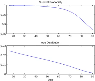
Figure 2: Calibrated Survival Probabilities and Population Age Profile.

5 Data and External Calibration

Tables 3 and 4, in the end of this section, summarize the parameters values of this exercise.

5.1 Demography

The population age profile {ϕt}Tt=1 depends on the population growth rate gn, the survival probabilities ψt+1 and the maximum age T that an agent can live. In this economy, a period corresponds to one year and an agent can live 75 years, so T = 75. Additionally, we assumed that an individual is born at age 16, so that the real maximum age is 90 years.

The data on survival probabilities are taken from IBGE’s 2011 mortality tables. Figure 2 plots these probabilities as they are used in the model. The population growth rate is chosen based on the average population growth from 2001 to 2011. This yields a gn equal to 0.01139.

Given the population’s growth rate and the survival probabilities, as mentioned before, one can calculate the population age profile. Figure 2 also plots the population age profile.

5.2 Preferences and Technology

The value ofβis chosen so that the capital-to-output ratio is between 2.5 and 3, values commonly used in the Macro literature for Brazil10. This resulted in a discount factor of 0.9751.

The consumption share in the utility,γ, takes the value of 0.468 to match the percentage of households that are currently working, taken from PNAD11, an annual cross-sectional household data survey published by IBGE. According to the survey, in the year of 2011, the participation rate was 79.83%.

Since it is quite difficult to find a reasonable way to calibrate the marginal utility coefficient of the public good12, for now, we will rely on Ferreira and do Nascimento (2005) and setǫ= 1₂. Therefore, we proceed assuming that there is imperfect substitution between private and public consumption.

10_{See Cavalcanti and dos Santos (2011), Glomm et al. (2009), dos Santos and Pereira (2010) and Ferreira and}

do Nascimento (2005).

11_{“Pesquisa Nacional por Amostra de Domic´ılios”}

12_{The empirical literature (Fiorito and Kollintzas (2004), Kwan (2006), Ni (1995), Pieroni and Aristei (2005)}

(26)

20 30 40 50 60 70 80 90 0

0.5 1 1.5 2 2.5 3

Leisure Cost

Age Leisure Cost

1

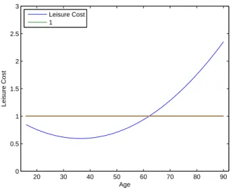
Figure 3: Cost Function.

As for the technology parameters, we will set the capital share in output as α = 0.43 and the depreciation rate at δ= 7.2%, as commonly used in the Macro literature.

5.3 Income Processes

In the model economy, all the heterogeneity among agents that is not related to the age, asset accumulation and working sector13 _{is captured by the idiosyncratic productivity of work,} _z

t. To calibrate the parameters of the AR(1) process, based on well established evidences for the US economy, we first set λz = 0.96. Then, we ran a simple Mincerian regression for the private sector workers, and assumed that the MSE equals the unconditional variance of z:

M SE =V ar(z) = σ2z

1−λ2

z. The regression is detailed in Column (2) of Table 2. This procedure

resulted in a variance of 0.0472. After determining the AR(1) parameters, we discretize it following Tauchen (1986), with 4 grid points.

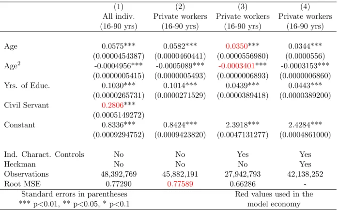
The wage premium of the public sector, θ, is calculated using 2011 PNAD data. We ran a Mincerian regression considering a dummy control variable for public sector workers. The definition of public servant used in this work is a statutory public worker. We do so because they are the ones subject to the retirement system we are modelling. Table 2, Column (1), summarizes the regression results. This procedure implies a public wage premium ofθ= 0.2806.

(27)

Table 2: Log of income per hour. Source: 2011 PNAD

(1) (2) (3) (4)

All indiv. Private workers Private workers Private workers (16-90 yrs) (16-90 yrs) (16-90 yrs) (16-90 yrs)

Age 0.0575*** 0.0582*** 0.0350*** 0.0344***

(0.0000454387) (0.0000460441) (0.0000556980) (0.0000556) Age2 -0.0004956*** -0.0005089*** -0.0003401*** -0.0003153***

(0.0000005415) (0.0000005493) (0.0000006893) (0.0000006860)

Yrs. of Educ. 0.1030*** 0.1014*** 0.0439*** 0.0443***

(0.0000265731) (0.0000271529) (0.0000389418) (0.0000389200)

Civil Servant 0.2806***

(0.0005149272)

Constant 0.8336*** 0.8424*** 2.3918*** 2.4284***

(0.0009294752) (0.0009423820) (0.0047131277) (0.0004861000)

Ind. Charact. Controls No No Yes Yes

Heckman No No No Yes

Observations 48,392,769 45,882,191 27,942,793 42,138,252

Root MSE 0.77290 0.77589 0.66286

-Standard errors in parentheses Red values used in the

*** p<0.01, ** p<0.05, * p<0.1 model economy

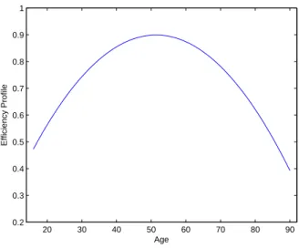
To calibrate the efficiency profile, {ηt}Tt=1, we follow Dos Reis and Zilberman (2014) and suppose the functional form: ηt =αη₁t+αη₂t2. As mentioned before, for each choice of labor,

Lt, the private worker will receive a total wage of yt =wezt+ηtLt. Dividing by Lt, taking logs and substituting zt, one gets:

log

yt

Lt

= logw+αη₁t+αη₂t2+λzzt−1+εz (4)

First, notice that we have an omitted variable problem, since we do not observe zt−1 on the data. Therefore, using ordinary least squares on the above expression would get us biased and inconsistent estimates ofαη₁ and αη₂, sincezt−1 is obviously correlated witht.

To alleviate this problem, we control for individuals characteristics such as different races, whether he is head of the household, has a farm job, what is the occupational sector the individual is working and whether he lives in urban area. The resulting values for αη₁ and αη₂

are 0.0350 and -0.0003401, respectively. The regression is detailed in Column (3), Table 2, and the age-efficiency profile used is shown in Figure 4.

Selection bias is another problem that arises in regression (4). It could be the case that only high-z agents keep on working after 60 years old. Since we only use strictly positive wage data, the coefficients may be overestimating the impact of age on wages for people older than 60 years old.

(28)

20 30 40 50 60 70 80 90 0.2

0.3 0.4 0.5 0.6 0.7 0.8 0.9 1

Efficiency Profile

Age

Figure 4: Efficiency Age Profile

The formal sector probability parameter, θF, is calibrated to match the size of the informal sector relative to Brazil’s population. According to IBGE, in 2011, approximately 22% of the population were working in the informal sector. Therefore, we setθF = 7.1.

5.4 Government Sector

To calibrate the cost function, we assumed a second-order polynomial form14_: _c

ap(t) =αap1 t2+

α₂apt+αap₃ . We calibrated the parameters αap₁ and αap₂ to match the average age in which individuals took the public exam and the amount of them who took it between 16-37 years old. The intercept, αap₃ is chosen to match the total amount of test takers in the economy. This resulted inαap₁ ,αap₂ and αap₃ equal 0.00061, -0.026 and 0.871, respectively.

Social security taxes of both public and private workers are taken directly from 2011 tax code. Public workers paid 11% of their income to the social security system. Private workers paid 8%, 9% or 11%, depending on their income, in the following manner:

τss(P F) =

  

 

8% if 0≤min(yt, ymax)≤ 1107₃₆₉₁..5274ymax 9% if 1107.52

3691.74ymax<min(yt, ymax)≤ 18453691..8774ymax 11% if 1845₃₆₉₁._.87₇₄ymax<min(yt, ymax)

(5)

Private retirees do not have any tax on their retirement benefits. Public retirees, on the other hand, must pay a 11% tax over the amount of their benefits that exceeds the maximum private benefit, y_max. Formally, they must pay 11% max{b−y_max,0} to the social security system.

The private sector labor income tax and the capital tax rate are chosen following the Macro literature for Brazil15. Therefore, we set them as τy(P) = 18% and τk = 15.5%. As done in Immervoll et al. (2006), we set the labor income tax of the public servants as τy(G) =

τy(P)

2 = 9%. The consumption tax rate is chosen to balance the government budget constraint in equilibrium.

14_{Other convex cost functions would serve as well. For instance,}

cap(t) =αap₁ eα

ap

2 t+αap₃ t. We chose a quadratic polynomial for simplicity. A constant cost function, cap= αap1 , would degenerate the test taker’s distribution (Figure 7), therefore we chose to put some heterogeneity with respect to t. The choice of not considering a

cap(t, z) was also for the sake of simplicity.

15_{See Paes and Bugarin (2006), Glomm et al. (2009), Glomm et al. (2005), Dos Reis and Zilberman (2014),}

(29)

The maximal value of a private pension, ymax, is chosen to match the ratio between the biggest pension paid to the private sector retirees with respect to the biggest pension paid to the public retirees, _maxmax{_{b_b₍(P_G)₎}_} = 0.123, taken from PNAD. The procedure resulted iny_max= 0.20. For the minimum wage, we set ymin = ₃₆₉₁545ymax. These values were obtained from comparing real minimum wage and social security benefits in 2011.

The fraction of the working population in the public sector, ¯NG, is set to be 3.762%, as it is calculated using data on sectoral occupation, also taken from PNAD. For the amount of public good produced by the government, since we are using a linear production function for the government so far, we necessarily haveYG= ¯NG= 3.762%.

5.5 External Calibration

Table 3 summarizes the external calibration procedure, as detailed above.

Table 3: External Calibration Summary

Parameter Description Value Source

{ψt}Tt=1 Survival probabilities - IBGE

gn Population’s growth rate 1.14% IBGE

σ Risk aversion 4.8 Issler and Piqueira (2000)

ǫ Public good ut. coef. 1₂ Ferreira and do Nascimento (2005)

α Capital share in output 0.43 Standard value

δ Depreciation 7.2% Standard value

λz Shock persistence 0.96 US economy

σ_z2 Shock variance 0.0472 PNAD

θ Public sector wage premium 0.2806 PNAD

αη₁ Age eff. profile coef. 0.0350 PNAD

αη₂ Age eff. profile coef. -0.0003401 PNAD

τss(m), ∀m SS income tax code - 2011 tax rates

τb(m), ∀m SS benefits tax code - 2011 tax rates

τy(P F) Private sector’s income tax 18% Literature

τy(G) Public sector’s income tax 9% Immervoll et al. (2006)

τk Capital tax 15.5% Literature

ymin Minimum wage ₃₆₉₁545ymax 2011 Min wage_{SS ceiling} ¯

NG Size of the govt. sector 3.762% PNAD

YG Public good 3.762% FG( ¯NG) = ¯NG

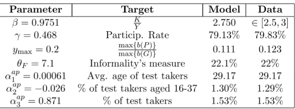
5.6 Internal Calibration

Table 4 summarizes the main features of the internal calibration procedure. In the end, as it can be seen, the calibration procedure was able to match closely the proposed targets.

Table 4: Internal Calibration Results

Parameter Target Model Data

β = 0.9751 K

Y 2.750 ∈[2.5,3]

γ = 0.468 Particip. Rate 79.13% 79.83%

y_max= 0.2 max_max{_{b_b(₍_GP₎)}_} 0.111 0.123

θF = 7.1 Informality’s measure 22.1% 22%

αap₁ = 0.00061 Avg. age of test takers 29.17 29.17

αap₂ =−0.026 % of test takers aged 16-37 1.30% 1.29%

(30)

20 40 60 80 0 0.1 0.2 0.3 0.4 0.5 0.6 0.7 0.8 0.9 1

Individuals Out of the Labor Force

Age 20 40 60 80

0 0.1 0.2 0.3 0.4 0.5 0.6 0.7 0.8 0.9 1 Public Servants Age Model Data

20 40 60 80 0 0.1 0.2 0.3 0.4 0.5 0.6 0.7 0.8 0.9 1

Total Private Workers

Age

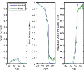
Figure 5: Agents’ Equilibrium Distribution in the Steady State.

6 External Validation

This section intends to externally validate our model. We are going to compare the outcome the modelling economy to the data in different aspects, mainly related to working and retirement decisions, the social security deficit and differences in wages paid in the public and private sectors.

First, Table 5 compares the aggregate distribution of the individuals generated by the model and in the data.

Table 5: Distribution of Individuals (%)

Retirement Public Private

Data 14.41 3.76 81.83

Model 16.69 3.71 79.41

As it can be seen, our model matches the aggregate distribution of individuals fairly well. It is worth noticing that the Public column is internally calibrated, once the government chooses ¯

q to have ¯NG workers in equilibrium. A more detailed analysis can be made by plotting, for each age, how individuals are distributed among the three sectors of the economy. Figure 5 represents the equilibrium distribution of individuals across sectors for the benchmark economy calibrated to the year of 2011.

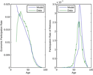
One can also look at the economic participation rate by age groups. Since the calibration procedure involves matching the total economic participation rate, it is interesting to see whether agents are behaving as in the data along the life-cycle. Table 6 reports our results.

Table 6: Participation Rate (%)

16-30 31-45 46-60 61-75 76-90 Data 28.27 27.70 18.57 4.82 0.48

Model 32.37 24.72 15.77 5.45 0.81

(31)

0 50 100 0

0.005 0.01 0.015 0.02 0.025

Economic Participation Rate

Age

Model Data

0 50 100

0 0.5 1 1.5 2 2.5 3 3.5x 10

−3

Participation Rate of Retirees

Age Model Data

Figure 6: Economic Participation Rate.

plotting the economic participation rate for each age, from 16 to 90. Figure 6 tells us that our model overestimates the number of young people who is choosing to work. Apart from the beginning of life, our model captures the labor offering decision fairly well.

The intuition for the distance between our model and the data is the following. First, all agents in the economy start with zero initial assets. Therefore they have to work early in life in order to compensate this lack of resources. Second, we are not modelling human capital accumulation nor schooling decisions. Most of the teenagers aged 16-18 in the data are probably ending their studies, preparing themselves to enter the market and still living with their parents. Therefore, the actual participation rate for young agents is low relative to what we have in both models.

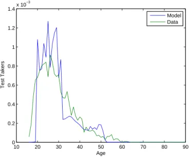
What can our model say about the agents that are taking the public exam? Figure 7 plots, for each age, what is the size of the test takers in the population and compare it to the data. Even though the average age, the total amount of people and the total amount of test takers between 16-37 years are internally calibrated, the disaggregated behavior of the agents is similar to what we observe in the data.

Figure 7 also tells us that there are two key moments during the life-cycle in which individual try their luck into becoming public servants. First, as expected, the agents try to enter the public sector as soon as possible. As it can be seen, there is a mass of agents with 20-30 years old that pay the cost of applying to the public sector. Once they fail in becoming public servants, they save some money and time contributed to the social security system working for the private sector (while their work productivity ηt is high), and then try again to enter the public sector later in life.

Another way of validating our model is to compare the social security deficit generated by the model with the real one. In 2011, the social security deficit was 1.6% of GDP16. In our model, the resulting social security deficit accounts for 2% of GDP.

If we look at the timing of retirement applications, we see that our model is able to reproduce the early retirement agents’ decisions quite well. Pereira (2013) shows that, in 2011, the average age in which Brazilian males claim for retirement under LC modality is 54.9 years old. In our modelling economy, agents apply for social security benefits under LC modality, on average,

16_{To calculate this deficit, we used data from Tafner et al. (2015) and from SIAFI -} _{Sistema Integrado de}

Administra¸c˜ao Financeira. We only considered revenues from the social security system, excluding revenues