Using ecological niche modeling to determine avian richness hotspots

(1)

Using ecological niche modeling to determine avian richness

hotspots

R. Mirzaei 1,_{*, M.R. Hemami}2_{, A. Esmaili Sari}3_{, H.R. Rezaei}4_{, A.T. Peterson}5

1_{Department of the Environment, Faculty of Natural Resources and Earth Sciences,}

University of Kashan, Kashan, Iran

2_{Department of Natural Resources, Isfahan University of Technology, Isfahan, Iran}

3_{Department of Environment, Faculty of Natural Resources and Marine Science, Tarbiat Modares}

University, Noor, Iran

4_{Gorgan University of Agricultural and Natural Resources, Gorgan, Iran}

5_{Biodiversity Institute, University of Kansas, Lawrence, Kansas, USA} DOI: 10.22034/gjesm.2017.03.02.002

ORIGINAL RESEARCH PAPER

Received 1 November 2016; revised 31 January 2017; accepted 20 February 2017; available online 1 March 2017

*Corresponding Author Email: rmirzaei@kashanu.ac.ir Tel.: +98 31 5591 3228 Fax: :+98 31 5591 3222

Note: Discussion period for this manuscript open until June 1, 2017 on GJESM website at the “Show Article”.

ABSTRACT: Understanding distributions of wildlife species is a key step towards identifying biodiversity hotspots and designing effective conservation strategies. In this paper, the spatial pattern of diversity of birds in Golestan Province, Iran, was estimated. Ecological niche modeling was used to determine distributions of 144 bird species across the province using a maximum entropy algorithm. Richness maps across all birds, and separately for rare and threatened species, were prepared as approximations to hotspots. Results showed close similarity between hotspots for all birds and those for rare birds; hotspots were concentrated in the southern and especially the southwestern parts of the province. Hotspots for threatened birds tended more to the central and especially the western parts of the province, which include coastal habitats. Based on three criteria, it is clear that the western part is the most important area of the province in terms of bird faunas. Despite some shortcomings, hotspot analysis could be applied to guide conservation efforts and provide

useful tool towards eficient conservation action.

KEYWORDS: Avifauna; Ecological niche, Golestan Province; Hotspots; Species distribution modeling; Threatened birds.

INTRODUCTION

Currently, protection of biodiversity is an important focus for scientists, decision makers, and the public, because biodiversity is a foundation of ecosystem function, providing the life-support system of the Earth (Walther et al., 2011, Wu et al., 2013, Xu et al., 2016, Waters et al., 2016). In recent years, areas with high biodiversity have been the focus of conservation

efforts. An important part of conservation biology is concerned with identifying biodiversity hotspots, a concept irst proposed by Mayer (1988), and now in broad use in various global, regional, and local efforts (Myers et al., 2000, Schouten et al., 2010, Wu

et al., 2013). Hotspots can be deined as areas with

the highest species richness of all species (Myers et al., 2000), or may focus on endemic species (Orme

(2)

132

R. Mirzaei et al.

areas highly affected by human activities (Brevik et al., 2015), such that conservation planning must be balanced against human needs and priorities.

In recent years, biodiversity mapping has seen important advances (Rodríguez et al., 2007), in which known occurrences of species are used to estimate ecological niches, which in turn are used to estimate potential distributions of species. Assessing overlap of potential distributions with protected areas constitutes a key step in gap analysis to optimize protection of biodiversity. Considering inancial limitations, protecting all biodiversity hotspots completely is generally impossible. Hence, assessing, analyzing, and comparing the importance of different biodiversity hotspots for conservation is essential to their protection. Analyzing the environmental and geographic extents of important biodiversity hotspots can offer a better understanding of their ecological characteristics (Hedo de Santiago et al., 2016, Ibáñez et al., 2016, Stavi et al., 2016). Understanding species’ distributions and the environmental factors that shape them is of great importance in conservation planning (Gray et al., 2006) and particularly to identifying hotspots (Ko et al., 2009). To this end, models based on associations between species’ presences and environmental variation are used (Koet al., 2009).

Early models were usually based on multivariate linear functions like linear/multiple regression and multiple discriminant analyses (Jose and Fernando, 1997). Such methods have limitations, which led to exploration of nonlinear responses and evolutionary

computing approaches (Elith et al., 2006). These models include genetic algorithms, ecological niche factor analysis, maximum entropy, and artiicial neural networks (Ko et al., 2009). These newer approaches provide ecologists with better tools for precise estimation of species’ niches and distributions (Stockwell, 2007). These models are known as “ecological niche models,” or “species distribution models” when the focus is on estimating the occupied distributional area of the species. The environmental variables used form a subset of the ecological niche dimensions of species (Peterson, 2001).

Avian diversity is under severe threat from human-caused habitat loss and fragmentation (Gaston et al., 2003). Identiication of high-value sites is critical

to maintaining avian diversity, given that resources available for conservation are limited (Turner et al., 2003). The emergence and ready availability of GIS and species distribution models has facilitated identiication of biodiversity hotspots. This study aimed to explore application of these approaches to mapping biodiversity hotspots across Golestan Province, Iran, as a step towards optimal design of conservation areas.

MATERIALS AND METHODS

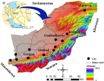
Golestan Province, with an area of 20,387 km2_{, is}

located along the southeastern edge of the Caspian Sea, covering 1.3% of the surface area of Iran (36°25’ to 38°8’ N and 53°50’ to 56°18’ E) (Fig. 1). Golestan Province has Turkmenistan to the north; Khorasan Province to the east; Semnan Province to the south and southeast;

(3)

133

and Mazandaran Province, the Bay of Gorgan, and the Caspian Sea to the west. This province includes plains, foothills, and mountains, and the climate ranges from arid and semiarid to mild and mountainous; average annual rainfall is 450 mm, reaching <200 mm in the north (Mirzaei, 2013).

7510 occurrence points for 243 bird species from across Golestan and Mazandaran provinces (Mirzaei, 2013) were used. Presence data were collected as part of a project of bird atlasing for northern Iran in 2012 and 2013. Field surveys of species were conducted for several different studies over this time period. Transects were surveyed visually by multiple ield teams at various times of the day. Georeferenced occurrence points were noted for all species identiied. Species with > 12 unique presence points were retained (Tognelli et al., 2011), leaving 144 species for analysis. Unfortunately, modeling several important parts of the avifauna of the province was not possible, as presence data were too few (e.g., Neophron percnopterus, Gypaetus barbatus). Initially, 29 variables were explored to summarize environmental variation across the province (Appendix 1). To avoid overitting owing to highly dimensional environmental spaces, using multicollinearity analysis, this set was reduced to 15 variables for analysis (Chatterjee and Hadi, 2006).

Occurrence data for each species were divided into calibration (75%) and evaluation (25%) sets. Background points were chosen randomly from across the study area. Ten runs and 1000 iterations were selected, and the average of the 10 runs was used as the inal map. This continuous map of suitability was

changed to binary using a 90% presence threshold: the suitability value whereby 90% of occurrence records were included (hereafter referred to as 90% PT). To evaluate models, receiver operating characteristic (ROC) curves were used; ROC shows the classiication eficiency of the model as the area under the ROC curve (AUC), independent of any particular threshold (Elith et al., 2006).

Species richness was then summarized in terms of total species richness, threat, and rarity. Overall species richness was calculated as the simple sum of the individual binary maps. For rarity, species were classiied into abundant (value 0), common (value 1), average (value 2), and rare (value 3). Nonnative species were given scores of 0. The third criterion was presence of threatened species, which we based on three criteria: IUCN, CITES, and national lists. IUCN near-threatened species got a score of 1, vulnerable species 2, and endangered species 3; species listed in Appendices1 and 2 of CITES got scores of 2 and 1, respectively. Finally, based on national criteria, protected and endangered species got scores 1 and 2, respectively. Final maps of threat and rarity were prepared as the weighted sums of individual binary maps.

RESULTS AND DISCUSSION

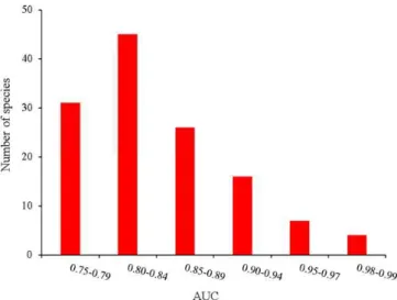
From the initial list of birds, 15 species were removed, as the predictions of their distributions were not robust (Fig. 2; AUC <0.75; Pearce and Ferrier, 2000, Elith, 2002, Pous et al., 2011). These species were Common Swift, Alpine Swift, Tawny Pipit, Tree Pipit, Eurasian Golden Oriole, Winchat, House

(4)

134

Identifying avian richness hotspots

Martin, Lesser Spotted Woodpecker, Alpine Chough, Eurasian Magpie, Eurasian Reed Warbler, Ortolan Bunting, Olivaceous Warbler, Eurasian Hobby, and Spotted Flycatcher. Hence, 129 species were included in our analyses (Appendix 2).

Species richness overall and richness of rare species had similar patterns (Fig. 3). Three distinct hotspots with highest species richness were identiied in Golestan Province: a) the southern and southwestern parts of the province, which are covered by forested mountains; b) the north-central parts of the province that include the Alagol, Ajigol, and Almagol wetlands, as well as Sooikom wetland and neighboring areas; and c) the western part of the province, which includes Gomishan Wetland and surrounding areas. The spatial pattern of threatened bird richness was different, seeming to follow habitat ecotones. Three hotspots were recognizable in this map: a) scattered areas in the central part of the province, b) the eastern sector of the province, and c) the western part, which includes signiicant wetland areas.

Hotspots have been developed based on three criteria and two thresholds (Fig. 4). Overall richness hotspots were closely similar to maps of rarity hotspots, with hotspots concentrated in the southern and southwestern parts of the province. Hotspots for threatened birds were in the central and, especially, western parts of the province, which consist of coastal habitats. Based on all three criteria, it becomes clear that the western areas are the most important part of the province in terms of species richness.

Finally, the results for the three hotspot criteria were combined to identify grid cells that were most valuable according to all three criteria. For the 30% criterion, several distinct clusters were identiied across the southern part of the province. For the more strict 20% criterion, smaller clusters were identiied, largely in the southwestern sectors of the province (Fig. 5). It is important to establish how much the three hotspot criteria overlapped: at the 30% criterion, 6.0% of the study area was “hot” for two criteria, and 0.4% of the study area was “hot” for three criteria. For the 20% criterion, overlap between two criteria was also around 2%, but overlap among all three criteria was only 0.02%.

Over recent decades, great advances have been made in development of predictive models of geographic and environmental distribution of species, rendering them useful tools for various applications (Rodríguez et al.,

2007). Using presence and absence data in ecology has been controversial. Some studies suggest that models that rely on presence data only make better predictions than those that also consider absence data (Ko et al.,

Fig. 3: Species richness of birds of Golestan Province, viewed in terms of total species richness, rare species richness, and threatened species richness

(5)

135 2009). One possible reason is that presence of a species in the area can be conirmed, but conirming absence of a species in the area can be quite complicated because identifying biological absence is not simple

or straightforward. An important caution regarding choice of environmental variables in these exercises is their relation to the speciic requirements of the species in question. If environmental variables are not those that constrain the habitat requirements of the species, model predictions will fail.

For example, the Magpie is an abundant species in Golestan Province, ostensibly with suficient presence points for modeling, yet the model’s eficiency in determining the distribution of the species was not satisfactory. One probable reason is that the environmental variables employed do not represent key predictors for this species. Further experimentation to identify appropriate environmental variables would

Fig. 4: Biodiversity hotspots for 129 bird species of Golestan Province, including the top 20% (red) and 30% (pink) of species richness

Fig. 5: Map of three hotspot criteria in Golestan Province; combined colors range from black (all three hotspot criteria fulfilled) to gray (only one of three hotspot criteria fulfilled). Left side is 30% criterion view, right side is

20% criterion view

Fig. 5: Map of three hotspot criteria in Golestan Province; combined colors range from black (all three hotspot criteria fulfilled) to gray (only one of three hotspot criteria fulfilled). Left side is 30% criterion view, right side is

20% criterion view

(6)

136

R. Mirzaei et al.

be necessary to be able to include this and other species in our analyses. Despite numerous studies (Liu et al., 2005, Jimenez-Valverde and Lobo, 2007, Pineda and Lobo, 2009), no agreement exists regarding the best method for choosing the threshold to change the continuous raw model outputs into binary maps (presence and absence). Most recent efforts have based threshold choice on omission only, but have allowed for some error (termed E) in the match between occurrence data (Urbina-Cardona and Loyola, 2008, Brito et al., 2009, Raes et al., 2009). More detailed discussion of these points is provided by Peterson et al. (2011).

The validity of every ecological niche modeling exercise depends upon the modeling methods, the quality and comprehensiveness of the occurrence data, and the quality and appropriateness of the environmental layers used as predictors in the model (Ron, 2005). Although the data used in this study are the best and most comprehensive information available for Iranian wildlife that have been collected on a regional or provincial level, they are by no means bereft of errors. Basically, one of the most important problems in such models is bias in sampling of species across geographic or environmental gradients (Barry and Elith, 2006). Such bias means that modeled relationships may be determined more by patterns in the sampling than by the physiology of the species; such problems will lead to spatial errors (Barry and Elith, 2006).

The dataset includes two main biases: a) temporal bias, as the ield activities did not cover the whole year, and rather were conined to April through August, thus they lack information on year-round distributions. Even sampling from all seasons may have information gaps, so data from several consecutive years are better, thus, that enough information can be gathered to permit modeling scarce species. b) Spatial bias, related to sampling areas is also important: although we tried to conduct our ield research in a systematic manner, and they were largely successful, ield research is never completely free of error and bias. The most important source of spatial bias lies in access to different parts of the province, a factor that depends critically on roads. By necessity, our sampling was concentrated in areas close to roads (Kadmon et al., 2003). Some measures were taken to reduce inluence of this bias: “distance from road variable” was discarded from environmental variables; spatial resolution of our maps was set to 1 km2_{; and data from adjoining Mazandaran}

Province were added to the data to improve sampling of

environments in our models.

This study treated only 129 bird species, and as such does not include all bird species of the province, being especially weak as regards winter resident species. Indeed, even some important species of the province, like Bearded Vulture, were omitted, as data were insuficient. As a result, one must keep in mind that our results cannot necessarily be generalized beyond these particular taxa. Many studies attest to the degree to which a single taxon is representative of overall biodiversity (Howard et al., 1998, Reyers et al., 2000): many have come to the conclusion that single higher taxa will rarely sufice, although some studies have had more promising results (Pinto et al., 2008). Hence, some caution is necessary in interpreting our results on the bird fauna of Golestan: they may not be appropriate substitutes for other groups, like mammals, reptiles, amphibians, plants, or invertebrates.

CONCLUSION

Analysis of hotspots for the birds of Golestan Province, as best areas in terms of biodiversity, was conducted using species distribution modeling and ecological niche modeling approaches. The results indicated higher diversity of birds in the southern areas of the province, which were covered by forested lands. To get better results, it is necessary to complement this information with information on other animals, such as mammals, reptiles, and amphibians, in future research. It is also necessary to prepare and integrate hotspots according to various scenarios and methods, so that results are closer to reality. Despite shortcomings, species distribution models have become important tools in conservation biology, as they provide better possibilities for estimating the real distributions of species compared to the previous distribution range maps. Thus, using distributional models improve information available to guide future conservation initiatives in Iran.

ACKNOWLEDGMENTS

Authors are grateful to Mr. Ghaemi, Mr. Shakiba, Mr. Hoseini, Mr. Hashemi, Mr. Cheraghi, Mr. Roshanian and Mr. Orschi, for their help during the ieldwork and data processing of the study performance.

CONFLICT OF INTEREST

(7)

137

ABBREVIATIONS

AUC Area under the curve

CITES

Convention on International Trade in Endangered Species of Wild Fauna and Flora

IUCN International Union for Conservation

of Nature

km2 _{Square kilometer}

Max. Maximum

Min. Minimum

mm Millimeter

NDVI Normalized difference vegetation index

PT Presence threshold

ROC Receiver operating characteristic

REFERENCES

Barry, S., Elith, J., (2006). Error and uncertainty in habitat models. J. Appl. Ecol., 43: 13-423 (410 pages).

Brevik, E.C., Cerdà, A.; Mataix-Solera, J.; Pereg, L.; Quinton, J.N.; Six, J.; Van Oost, K., (2015). The interdisciplinary nature of soil. Soil., 1: 117-129 (13 pages).

Brito, J.C.; Acosta, A.L.; A´lvares, F.; Cuzin, F., (2009). Biogeography and conservation of taxa from remote regions: An application of ecological-niche based models and GIS to North-African Canids. Biol. Conserv.,142: 3020-3029 (10 pages).

Chatterjee, S.; Hadi, A., (2006). Regression analysis by example. John Wiley and Sons, New York, (416 pages).

Elith, J., (2002). Quantitative methods for modeling species habitat: Comparative performance and an application to Australian plants. In: Ferson S,Burgman M (eds) Quantitative methods for conservation biology, Springer,New York, pp 39-58 (20 pages). Elith, J.; Graham, C.; Anderson, R.P.; Dudik, M.; Ferrier, S.; Guisan,

A.; Hijmans, R.J.; Huettmann, F.; Leathwick, J.R.; Lehmann, A.; Li, J.; Lohmann, L.G.; Loiselle, B.A.; Manin, G.; Moritz, C.; Nakamura, M.; Nakazawa, Y.; Overton, J.M.C.; Peterson, A.T.; Phillips, S.J.; Richardson, K.S.; Scachetti-Prereira, R.; Schapire, R.E.; Sobero´n, J.; Williams, S.; Wisz, M.S.; Zimmermann, N.E. ,(2006). Novel methods improve prediction of species distributions from occurrence data. Ecography., 29: 129-151 (23 pages). Gaston, K.J.; Blackburn, T.M.; Goldewijk, K.K., (2003). Habitat

conversion and global avian biodiversity loss. Proc. R. Soc. B., 270: 1293-1300 (7 pages).

Giovanelli, J.G.R.; De Siqueira, M.F.; Haddad, C.F.B.; Alexandrino, J., (2010). Modeling a spatially restricted distribution in the Neotropics: How the size of calibration area affects the

performance of ive presence-only methods. Ecol. Model., 221:

215-224 (10 pages).

Gray, D.; Scarsbrook, M.P.; Harding, J.S., (2006). Spatial biodiversity patterns in a large New Zealand braided river. N. Z. J. Mar. Freshwater Res., 40: 631-642 (12 pages).

Grenyer, R.; Orme, C.D.L.; Jackson, S.F.; Thomas, G.H.; Davies, R.G.; Davies, T.J.; Jones, K.E.; Olson, V.A.; Ridgely, R.S.; Rasmussen, P.C.; Ding, T.S.; Bennett, P.M.; Blackburn, T.M.; Gaston, K.J.; Gittleman, J.L.; Owens, I.P.F., (2006). Global distribution and conservation of rare and threatened vertebrates.

Nature., 444: 93-96 (4 pages).

Hedo de Santiago, J.; Lucas-Borja, M.E.; Wic-Baena, C.; Andrés-Abellán, M.; de lasHeras, J., (2016). Effects of thinning and induced drought on microbiological soil properties and plant species diversity at dry and semiarid locations. Land Degrad. Dev., 27(4): 1151-1162 (12 pages).

Howard, P.C.; Viskanic, P.; Davenport, T.R.B.; Baltzer, M.; Dickinson, C.J.; Lwanga, J.S.; Matthews, R.E.; Balmford, A., (1998). Complementarity and the use of indicator groups for reserve selection in Uganda.Nature., 394: 472-475 (3 pages). Ibáñez, J.J.; Pérez-Gómez, R.; Brevik, E.C.; Cerdà, A., (2016).

Islands of biogeodiversity in arid lands on a polygons map study: Detecting scale invariance patterns from natural resources maps. Sci. Total Environ., 573: 1638-1647 (10 pages).

Jime´nez-Valverde, A.; Lobo, J.M., (2007). Threshold criteria for conversion of probability of species presence to either–or presence–absence. Acta Oecol., 31: 361-369 (9 pages).

Jose, M.P.; Fernando, T., (1997). Prediction of functional

characteristics of ecosystem: a comparison of artiicial neural

networks and regression models. Ecol. Model., 98:173-186 (14 pages).

Kadmon, R.; Farber, O.; Danin, A., (2003). A systematic analysis of factors affecting the performance of climatic envelope models. Ecol. Appl., 13:853-867 (15 pages).

Ko, C.Y.; Lin, R.S.; Ding, T.S.; Hsieh, C.H.; Lee, P.F., (2009). Identifying biodiversity hotspots by predictive models: A case study using Taiwan’s endemic bird species. Zool. Stud., 48: 418-431(14 pages).

Liu, C.; Berry, P.M.; Dawson, T.P.; Pearson, R.G., (2005). Selecting thresholds of occurrence in the prediction of species distributions. Ecography, 28: 385-393 (9 pages).

Mirzaei, R., (2013). Determination of suitable areas for the conservation of birds based on spatial distribution of environmental threats and species diversity in Golestan Province. Dissertation, Tarbiat Modares University publication, (127 pages).

Myers, N.; Mittermeier, R.A.; Mittermeier, C.G.; da Fonseca, G.A.B.; Kent, J., (2000). Biodiversity hotspots for conservation priorities. Nature, 403: 853-858 (6 pages).

Orme, C.D.L.; Davies, R.G.; Burgess, M.; Eigenbrod, F.; Pickup, N.; Olson, V.A.; Webster, A.J.; Ding, T.S.; Rasmussen, P.C.; Ridgely,

R.S.; Stattersield, A.J.; Bennett, P.M.; Blackburn, T.M.; Gaston,

K.J.; Owens, I.P.F., (2005). Global hotspots of species richness are not congruent with endemism or threat. Nature, 436: 1016-1019 (4 pages).

Pearce, J.; Ferrier, S., (2000). Evaluating the predictive performance of habitat models developed using logistic regression. Ecol. Model., 133: 225-245 (21 pages).

Peterson, A.T., (2001). Predicting species’ geographic distributions based on ecological niche modeling. The Condor., 103: 599–605 (7 pages).

Peterson, A.T.; Soberon, J.; Pearson, R.G.; Anderson, R.P.; Martinez-Meyer, E.; Nakamura, M.; Araujo, M.A., (2011). Ecological niches and geographic distributions (MPB-49). Princeton University Press, Princeton, (328 pages).

Pineda, E.; Lobo, J.M., (2009). Assessing the accuracy of species distribution models to predict amphibian species richness patterns. J. Anim. Ecol., 78: 182-190 (9 pages).

(8)

138

Pous, P.D.; Beukema, W.; Weterings, M.; Dummer, I.; Geniez, P., (2011). Area prioritization and performance evaluation of the conservation area network for the Moroccan herpetofauna: a preliminary assessment. Biodivers. Conserv., 20: 89-118 (30 pages). Raes, N.; Roos, M.C.; Slik, J.W.F.; Loon, E., TerSteege, H., (2009).

Botanical richness and endemicity patterns of Borneo derived from species distribution models. Ecography, 32: 180-192 (13 pages). Reyers, B., van Jaarsveld, A.S., Krüger, M., (2000). Complementarily

as a biodiversity indicator strategy. Proc. R. Soc. B., 267: 505-513 (9 pages).

Rodríguez, J.P.; Brotons, L.; Bustamante, J.; Seoane, J., (2007). The application of predictive modeling of species distribution to biodiversity conservation. Divers. Distrib., 13: 243-251(9 pages). Ron, S.R., (2005). Predicting the distribution of the amphibian

pathogen Batrachochytriumdendrobatidis in the New World. Biotropica., 37: 209-221 (12 pages).

Schouten, M.A.; Barendregt, A.; Verweij, P.A.; Kalkman, V.J.; Kleukers, R.M.J.C.; Lenders, H.J.R.; Siebel, H.N., (2010).

Deining hotspots of characteristic species for multiple taxonomic

groups in the Netherlands. Biodivers. Conserv., 19: 2517-2536 (20 pages).

Stavi, I.; Rachmilevitch, S.; Yizhaq, H., (2016). Small-scale geodiversity regulates functioning, connectivity, and productivity of shrubby, semi-arid rangelands. Land Degrad. Dev., doi:10.1002/ ldr.2469, (6 pages).

Stockwell, D., (2007). Niche modeling. Chapman and Hall/CRC Press, Boca Raton, (199 pages).

Tognelli, M.F.; Abba, A.M.; Bender, J.B.; Seitz, V.P., (2011). Assessing conservation priorities of xenarthrans in Argentina. Biodivers. Conserv., 20: 141-151 (11 pages).

Wu, T.Y.; Walther, B.A.; Chen, Y.H.; Lin, R.S.; Lee, P.F., (2013). Hotspot analysis of Taiwanese breeding birds to determine gaps in the protected area network. Zool. Stud., 52: 1-29 (29 pages). Walther, B.A.; Larigauderie, A.; Loreau, M., (2011). Diversities:

Biodiversity science integrating research and policy for human well-being. In: Brauch HG, Spring ÚO, Mesjasz C (eds.) Coping with global environmental change, disasters and security- threats, challenges, vulnerabilities and risks, Springer-Verlag, Berlin, pp 1235-1248 (14 pages).

Waters, C.M.; Orgill, S.E.; Melville, G.J.; Toole, I.D.; Smith, W.J., (2016). Management of grazing intensity in the semi-arid rangelands of southern Australia: Effects on soil and biodiversity. Land Degrad. Dev., doi:10.1002/ldr.2602 (30 pages).

Turner, W.; Spector, S., Gardiner, N.; Fladeland, M.; Sterling, E.; Steininger, M., (2003). Remote sensing for biodiversity science and conservation. Trends Ecol. Evol., 18: 306-314 (8 pages). Urbina-Cardona, J.N.; Loyola, R.D., (2008). Applying niche-based

models to predict endangered-hylid potential distributions: Are neotropical protected areas effective enough? Trop. Conserv. Sci., 1: 417- 445 (29 pages).

Xu, L.; Cao, Y.; Li, W.; Cheng, Y.; Qin, T.; Zhou, Y.; Liu, F., (2016). Maintain spatial heterogeneity, maintain biodiversity: A seed bank study in a grazed alpine fen meadow. Land Degrad. Dev., doi:10.1002/ldr.2606 (30 pages).

1

Appendix1: Environmental predictors available for this study

No. Variable Data type Scale/Resolution Source of Data

1 Elevation Continuous 90 m USGS/SRTM

2 Aspect Categorical 90 m USGS/SRTM

3 Slope Continuous 90 m USGS/SRTM

4 NDVI Continuous 250 m http://modis.gsfc.nasa.gov/

5 Distance to agriculture area Continuous 1:50000 Office of Natural Resources of Golestan

6 Distance to forest Continuous 1:50000 Office of Natural Resources of Golestan

7 Distance to settlement area Continuous 1:50000 Office of Natural Resources of Golestan

8 Distance to water body Continuous 1:50000 Office of Natural Resources of Golestan

9 Distance to river Continuous 1:50000 Office of Natural Resources of Golestan

10 Land use Categorical 1:50000 Office of Natural Resources of Golestan

11 Isothermally Continuous 1 km2 _{URL:http://worldclim.org}

12 Mean temperature of wettest quarter Continuous 1 km2 _{URL:http://worldclim.org}

13 Mean temperature of driest quarter Continuous 1 km2 _{URL:http://worldclim.org}

14 Precipitation seasonality Continuous 1 km2 _{URL:http://worldclim.org}

15 Precipitation of warmest quarter Continuous 1 km2 _{URL:http://worldclim.org}

16 Annual mean temperature Continuous 1 km2 _{URL:http://worldclim.org}

17 Mean diurnal range Continuous 1 km2 _{URL:http://worldclim.org}

18 Temperature seasonality Continuous 1 km2 _{URL:http://worldclim.org}

19 Max.temperature of warmest month Continuous 1 km2 _{URL:http://worldclim.org}

20 Min.temperature of coldest month Continuous 1 km2 _{URL:http://worldclim.org}

21 Temperature annual range Continuous 1 km2 _{URL:http://worldclim.org}

22 Mean temperature of warmest quarter Continuous 1 km2 _{URL:http://worldclim.org}

23 Mean temperature of coldest quarter Continuous 1 km2 _{URL:http://worldclim.org}

24 Annual precipitation Continuous 1 km2 _{URL:http://worldclim.org}

25 Precipitation of wettest month Continuous 1 km2 _{URL:http://worldclim.org}

26 Precipitation of driest month Continuous 1 km2 _{URL:http://worldclim.org}

27 Precipitation of wettest quarter Continuous 1 km2 _{URL:http://worldclim.org}

28 Precipitation of driest quarter Continuous 1 km2 _{URL:http://worldclim.org}

29 Precipitation of coldest quarter Continuous 1 km2 _{URL:http://worldclim.org}

⃰ The first 15 variables were selected for modeling