Classification model of arousal and valence mental
states by EEG signals analysis and Brodmann
correlations
Adrian
Rodriguez
Aguin˜aga
and
Miguel
Angel
Lo´pez
Ram´ırez
InstitutoTecnolo´gicodeTijuana
CalzadadelTecnolo´gicoS/N,Toma´sAquino,22414 Tijuana, B.C.Me´xico
Mar´ıa
del
Rosario
Baltazar
Flores
InstitutoTecnolo´gicode Leo´n Av.Tecnolo´gicoS/N
IndustrialJulia´ndeObrego´n,37290 Leo´n, Gto.Me´xico
Abstract—This paper proposes a methodology to perform emotional states classification by the analysis of EEG signals, wavelet decomposition and an electrode discrimination process, that associates electrodes of a 10/20 model to Brodmann regions and reduce computational burden. The classification process were performed by a Support Vector Machines Classification process, achieving a 81.46 percent of classification rate for a multi-class problem and the emotions modeling are based in an adjusted space from the Russell Arousal Valence Space and the Geneva model.
Keywords—Emotions; Affective Computing; EEG; SVM; Wavelets;
I. INTRODUCTION
The development of technologies that allow interaction between a user and a computer in a more natural way, has been one of biggest challenges in recent decades.
Since Rosalind Picard founded the Affective Computing Group at MIT and propose theories to establish a better understanding of the impact of technology on the emotional states [1], a wide range of important developments focused in the human-machine interaction have been developed; being one of the most relevant the analysis of emotional states, due the great importance of emotions in our daily communication.
To date many techniques to analyzing the physiological expressions of an emotion have been developed; however, most of them are susceptible to be manipulated by users and provide unreliable information. One of the main proposals to resolve this problems, are the analysis of bio-medical signals (biosignals), such as heart rate, breathing rate and the behavior of neural signals that properly processed can be an important and reliable information source [2]; being the brain signal analysis, one of the techniques that has gained an increased demand in the past decades, due the recent developments in Brain Computer Interfaces (BCI), signal processing and pattern recognition algorithms facilitates the analysis, development and implementation of affective technologies. Also previous efforts to perform emotional states recognition, has been reached up to 80% of classification rates (Table I), promising results if we consider that a person can recognize an emotional state from another only the 88% of the time.
This paper presents a strategy for recognition and clas-sification of emotional states through analysis of electroen-cephalography (EEG) signals and a data reduction strategy based on the correlation between electrodes and a bounded region delimited by a Brodmann model analysis.
A. Related work
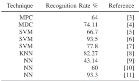
Recent advances in the analysis of biological signals achieves promising results as presented in Table I.
TABLE I: Previous emotion recognition developments and it recognition rate.
Technique Recognition Rate % Reference
MPC 64 [3]
MDC 74.11 [4]
SVM 66.7 [5]
SVM 93.5 [6]
SVM 77.8 [7]
KNN 82.27 [8]
NN 43.14 [9]
NN 60 [10]
NN 93.3 [11]
Many of this research’s achieves more than 88% of recog-nition rate, however, by performing binary classifications task or employing physiological characteristics as reference, since the associated to biological signals analysis shows a significant decrements in the recognition rate. Although a wide variety of techniques to perform classification are being implement to date, SVM and NN has shown the best performance.
Section II, describes a proposed emotion characterization model to perform a multidimensional classification process; Section III, describes a proposed strategy to reduce data in an EEG analysis by establishing a bounded regions of an electrode correlations to Brodmann regions and the features extraction and arrangement; Section IV, describes the configuration for the classification process and the implemented methodology to perform the experimentation processes; Section V, presents the results obtained by implementing the proposed strategies and Section VI, discusses the conclusions of this work.
II. EMOTIONS
Define a concept of emotion, could be a notorious problem without a proper review in the psychology advances.
Since we are proposing a classification task which involves a systematic process, the adopted definition of emotion has to satisfy this constraint. Klaus R. Scherer, define emotions asan episode of interrelated, synchronized changes in the states of all or most of the five1 organismic subsystems 2 in response to the evaluation of an external or internal stimulus event as relevant to major concerns of the organism[12].
However, the high diversity of theories associated to emo-tional states, implies that a very extensive endeavors must be performed just to pose an appropriate model to perform an adequate classification space. Fortunately Paul Ekman, Wallace Friesen, James Russell and Klaus R. Scherer propose theories that could be used to overcome most of this issues.
Ekman and Friesen propose the big six and the micro-expressions theory which generalize emotional gestures and provide tags to emotional states [13], Russell proposed an Arousal and Valence Space (AVS), where an emotional state could be represented as combination levels [14] and the Geneva model to provide a higher abstraction level by the addition of a dominance parameter to the AVS [12]. The classification classes are then conformed by referencing each experimental case to a certain emotion, with the following parameters:
• Arousal: ranges from inactive (e.g. uninterested,
bored) to active (e.g. alert, excited).
• Valence: ranges from unpleasant (e.g. sad, stressed) to pleasant (e.g. happy, elated).
• Dominance: ranges from a helpless and weak feeling
(without control) to an empowered feeling (in control of everything).
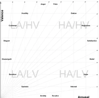
The proposed space 3 are configured as in Figure 1, to establish a four class problems defined as high arousal and high valence ([HA-HV] Happiness-Elation), high arousal and low valence ([HA-LV] Relax-Calm ), low arousal and high valence ([LA-HV] Boredom-Sadness) and low arousal and low valence ([LA-LV] Hostility-Anger), combinations.
A. Data characterization
The lack of benchmarks databases, is another important challenge in the emotional states classification process due that standardized databases as the International Affective Pic-ture System Digitized (IAPS) and the International Affective Digital Sounds (IADS) [15] [16], can only be employed to perform experimental setups and databases as the bu-3DFE, PhysioNet, iBUG project and DEAP dataset, which provides an experimental generalization due it are conformed from
1Information processing (CNS), Support (CNS, NES, ANS), Executive (CNS), Action (SNS), Monitor (CNS.)
2(CNS), central nervous system; (NES), neuro-endocrine system; (ANS), autonomic nervous system; (SNS), somatic nervous system. The organismic subsystems are theoretically postulated functional units or networks.
3This model do not consider the dominance parameter to keep the experi-ment in an four class problem.
Fig. 1: AVS model: The emotion distribution provided by the Russell AVS and the discrete tags by the Ekman model.
biological signals of a specific group of participants are not standardized.
• bu-3DFE [17]: a database by GAIC lab of is a collec-tion of facial expressions records.
• PhysioNet [18]: a very wide a collection of bio sig-nals provided by the National Institute of Biomedical Imaging and Bioengineering.
• The iBUG project [19]: a set of databases of the
human behavior analysis through a bio signals char-acterization recompiled by the Intelligent Behavior Understanding Group.
• Database for Emotion Analysis using Physiological
Signals (DEAP)[20]: is a collection of biomedical information from thirty two participants submitted to emotional stimulus.
To perform our classification task, we implement the DEAP dataset, which is up to our best knowledge the most complete database and are developed under the specific purpose of record the psychological responses of an emotion in arousal and valence levels. Also DEAP is already related to several other research projects [21] [22] [23] [24].
III. SIGNAL CONDITIONING
The large amounts of data associated to an EEG classi-fication process are also an important issue to be addressed and to handle whit it, a strategy that reduces the processed data by implementing an electrode discrimination process and a reduction of the spectral information by a frequency bands cutoff, are presented.
A. Brodmann analysis
Several researches has sought the establishment of a region based criteria which relates emotional activity to brain regions, an many of them suggest an association between the occipital and temporal cortex regions with emotional processes4.
The proposed strategy suggested in this work, establish a relationship between cortex regions an its relevancy in the classification (TableII).
Figure 2.
TABLE II: Boadmann association regions
Process Brodmann regions Cortex regions
Visual 17,18,19,20,21,37. Temporal lobe Occipital lobe Auditory 22,41,42. Temporal lobe Sensitive 1,2,3,4,5,7,22,37,39,40 Parietal lobe
Motor 4,6,44,9,10,11,45,46,47 Temporal lobe Frontal lobe
Also Table III, presents the association between electrodes to the associated regions an its correlation to conform a region based model, presented in Figure 2.
TABLE III: Brodmann regions and it associated electrodes
Associated region Electrode
Frontal Temporal 7 F7 Frontal cortex 5 FC5 Parieto Temporal 7 T7
Parietal cortex 5 CP5 Parieto Occipital 7 P7 Parieto Occipital 3 P3 Occipital 1 O1 Occipital 2 O2 Parieto Occipital 4 P4 Parieto Occipital 8 P8 Frontal cortex 6 C6 Temporal 8 T8 Frontal cortex 5 C5 Frontal Temporal 8 F8 Parietal cortex 6 CP6
This strategy only considers only fifteen electrodes from a differential 10/20 model and achieves a reduction of 38.5% of the total processed data.
B. Filtering
Noise and crosstalking effects are another important prob-lem to be addressed to identify a specific behavior EEG signals, an a wide range of signal processing techniques must be implemented just to handle with this problem [2][25]. EEG noise are generally related to instrumentation and physiological activity as the vascular, muscular or ocular movements and to attenuate this, a derivative of a surface LaPlacean filter (SL) suggested by M. Murugappan were implemented to lead a proper filtering process [26] [27]. This technique filters out the signals originated outside of the skull and emphasizing the
4Encompassing the hypothalamus, pituitary gland, amygdala and hippocam-pus.
Fig. 2: Selected electrodes as primary electrodes, this associa-tion are modeled with the 10/20 Biosemis system as reference.
electrical activity that occurs near an electrode by attenuating EEG activity and improving the spatial resolution of the signals, when it became common to all electrodes.
Xnew=X(t)−1/NE NE
X
i=1
Xi(t), (1)
whereXnewis the filtered signal,X(t)the raw signals and
NE the number of neighbor electrodes.
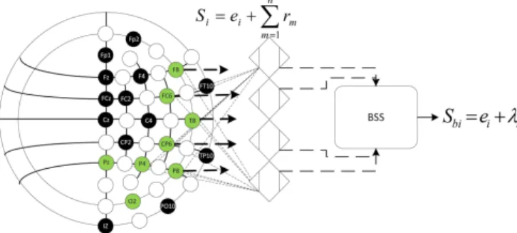
Also a Independent Component Analysis Blind Source Separation technique (ICA-BSS) were implemented to in-clude the uncorrelated information associated by the electrode discriminant process. This process also reduces redundancy and preserve references of the uncorrelated electrodes, by the decomposition of the signal into its constituent independent componentsXnew, considering a multi-channel signal problem defined as y(n)and the constituent components of the signal as yi(n), then
PY(y(n)) = i=1 Y
m
py(yi(n)) ∀n, (2)
wherePY is the probability distribution set,py(yi(n))are the marginal distributions andmis the number of independent components, performed over all the of electrodes (Figure 3).
To consider all the mixing structure process are necessary to estimates all the independent sources from the signal and for most cases this information are unavailable, and the as-sumption that this mixing process occurs as an instant case are widely accepted in the analysis of biological signals such as EEG where the signals are composed by a narrow bandwidth and a low sampling frequency5, the formulating BSS model
are modeled as
5This case assumes that signals reach the sensors at the same time.
Fig. 3: Si are the overlay sensor signals,ei are the electrodes references and Pnm=1rm is the attached signal of the elec-trodes. Sbi is the reference signal of a electrode after the filtering process, where ei is the electrode signal of a single electrode plus the λi remaining overlay signals of the non-primary electrodes. The main approach is that the reference energy at the focal points of the sensor will be increased, so that by using a process of BSS, may obtain independent vectors corresponding to each region.
z=Hs(n) +v(n), (3)
H are the mixing matrix,v(n) denotes the signal source
vectors and z is a mxn matrix from n samples, from a
m-dimensional array of electrodes activity.
C. Rhythms
The frequency bands associated to brain activity are de-nominated as rhythms (Table IV), and several studies suggest that are associated to a specific mental tasks; as another measure to perform signal conditioning a band pass filter of 0.5 Hz to 47 Hz, were implemented to consider only the frequencies of rhythms [25] [28].
TABLE IV: Brain rhythms [25].
Rhythms Frequency band (Hz)
Delta 0.5 to 4 Theta 4 to 8 Alpha 8 to 12
Mu 8 to 13 Beta 12 to 30 Gamma >30
D. Feature extraction
1) Wavelet decomposition: Despite the fact that to date, many techniques to perform EEG feature extraction have been developed; Wavelet Transform (WT), still are one of the most reliable feature extraction methodology in the EEG analysis [29] [27]; one of the most important aspects of the WT, is that transformation coefficients can be employed directly as features for the classification problem and unlike the Fourier transform it provides a commitment between the spatial and temporal information of the signal6, which are very useful in
6The time-frequency representation are performed by a set of filters, that limits the frequency domain by half and decompose the signal into approximation coefficients (AC) and detail coefficients (DC) and this process are performed by iterative and complementary filters
the analysis of biological signals.
Also WT handles with the non-stationary nature of the EEG signals by expanding, contracting and shifting a functionψa,b
called ”mother” wavelet, defined by as
ψa,b(t) = √1 aψ
t−b
a
a, b∈R, a >0, (4)
Rare in a wavelet space andais a scaling factor,b is the shifting factor.
Due EEG signals are non-stationary and their local waves are often spatially variant to decompose a signal into the elementary building blocks. WT allows a well localized in time and frequency due small scales reflects the high frequency components of the signal and large scales reflects the low fre-quency components of the signal, allowing the representation of the temporal features of a signal at different resolution [30].
The selection of an appropriate wavelet for a given signal, still implies an extensive search; to perform the presented feature extraction Daubechie 6 (DB6), were selected due it shows the best performance in a heuristic experimental task and also satisfy the following admissibility condition to handle whit the non-stationary propriety of EEG
Cψ=
Z ∞
−∞
|Ψ(ω)|2
ω dω <∞, (5)
whereΨ(ω), is the Fourier transform ofψa,b(t).
2) Approximation and detail based features: The WT de-scribes signal in terms of coefficients by representing their energy content in a specified frequency region and this coeffi-cients conforms the classification arrangements.
This signalf(t)can be decomposed as
f(t) =X j
X
k
dj,kψj,k(t) =X j
fj(t), (6)
where j,k ∈ Z and ψ(t) is a mother Wavelet and the
coefficientsdj,k is the inner product
dj,k=hf(t), ψj,k(t)i= √1 2j
Z
f(t)ψ(2−j
t−k)dt, (7)
From the wavelet coefficientsdj,k, the energy of the details off at levelj can be expressed as
Ej =X k
d2
j,k. (8)
If the total energy of the details is denoted asEt=P jEj,
then the percentile energy corresponding at levelj is:
εj =Ej
Et ×100, (9)
The levelj is associated with frequency band,∆F, given by:
2−j−1
Fs6∆F62−j
Fs, (10)
whereFsis the sampling frequency.
IV. CLASSIFICATION A. Experimental setup
Figure 4, presents the four classes distribution generated by a statistic distribution of from the evoked potential to describes each experiment case. The classes are conformed by sets of
2 4 6 8 2 4 6 8 2 4 6 8 Valence Arousal Dominance
Fig. 4: Evoked potentials distribution arrangement base on the
¯
xEP of the thirty two participants.
ten experimental setups.
1) Cases: A sub-cases configuration were proposed to evaluated the performance of this classification strategy; under distinct information configurations, conformed by an arrange-ments selection of the three most representative experimental cases, as presented in Figure 5.
1 2 3 4 5 6 7 8 9
1 2 3 4 5 6 7 8 9 1 2 3 4 5 6 7 8 9 10 11 12 13 14 15 16 17 18 19 20 21 22 23 24 25 26 27 28 29 30 31 32 33 34 35 36 37 38 39 40 Arousal Valence EP distribution
Fig. 5: Most representative experimental cases associated to each class, selected by a Mahalanobis distance.
This configuration shows the performance obtained under distinct stimulus over all the participants, and to ensure that each of this arrangements contains the information of different experimentation trials constructed under the following config-uration:
• Case A: Information of a the experimental cases
3,12,28 and 32.
• Case B: Information of a the experimental cases
2,15,21 and 35.
• Case C: Information of a the experimental cases
10,17,23 and 38.
• Case D: Mixing of the cases A,B and C.
B. SVM configuration
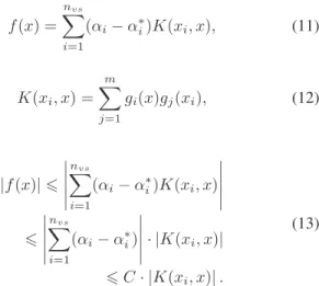
1) Selection of parameter C: In [31], to chose an optimal of regularization parameter C can be derived from standard parameterization of SVM solution given by expressions
f(x) = nvs
X
i=1
(αi−α∗
i)K(xi, x), (11)
K(xi, x) = m X
j=1
gi(x)gj(xi), (12)
|f(x)|6
nvs X i=1
(αi−α∗
i)K(xi, x) 6 nvs X i=1
(αi−α∗ i)
· |K(xi, x)|
6C· |K(xi, x)|.
(13)
Further in [31], use kernel functions bounded in the input domain. To simplify presentation, assume RBF kernel function
K(xi, x) =exp −
x−x2
2p2
!
, (14)
so that K(xi, x) 6 1 . Hence it obtain the following upper bound on SVM regression function:
|f(x)|6 C·nvs)
, (15)
Expression (15) is conceptually important, as it relates regularization parameterCand the number of support vectors, for a given value ofε. However, note that the relative number of support vectors depends on theε-value. In order to estimate
the value of C independently of (unknown) svn, one can
robustly let C ≥ f(x) for all training samples, which leads to setting Cequal to the range of response values of training data. However, such a setting is quite sensitive to the possible presence of outliers, as propose to use it instead the following prescription for regularization parameter:
C=max(|y¯+ 3σy|,|y¯−3σy|), (16)
wherey¯is the mean of the training responses (outputs), and
σ y is the standard deviation of the training response values. Prescription can effectively handle outliers in the training data. In practice, the response values of training data are often scaled so that y¯= 0; then the proposedC is3σy.
2) Selection of ε: It is well-known that the value of ε
should be proportional to the input noise level, that is ε∞σ. It assume that the standard deviation of noise σis known or can be estimated from data . However, the choice of εshould also depend on the number of training samples. From standard statistical theory, the variance of observations about the trend line (for linear regression) is:
σ2
y/x∞
σ2
n. (17)
This suggests the following prescription for choosingε:
ε∞√σ
n. (18)
Based on a number of empirical comparisons, it found that works well when the number of samples is small, however for large values of n prescription yieldsε-values that are too small. Hence we propose the following (empirical) dependency:
ε=τ σ r
ln(n)
n . (19)
Based on empirical tuning, the constant valueτ= 3 gives good performance for various data set sizes, noise levels and target functions for SVM regression. Thus expression is used in all empirical comparisons as presented in [31].
V. RESULTS
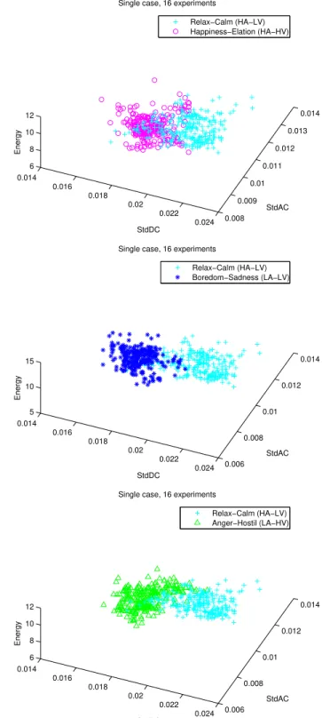
The resulting schemes from the implementation of the pro-posed discrimination scheme and BSS processes are presented in Figures 6, 7 and 8, where a insight of the behavior of the wavelets coefficients, between the possible combination of emotional could be observed with out the classification process.
Figure 6, presents the characteristics distribution, obtained by the implementation of the proposed strategy by employing the relaxed state (High arousal and low valence(relaxed or calm)) as reference and it comparative to states as anger (Low arousal and high valence (angry or rage)), happiness (High arousal and high valence (happiness or joy)) and sadness (Low arousal and low valence (boredom or sadness).
Figure 7, provides a features distribution representation that implements happiness state as reference to perform a comparative of it behavior with sadness and anger related features and Figure 8, presents the remaining combination of classification process (sadness and anger).
Also the combinations of a greater amount of interlocking elements, to observe the difficulty of the classification problem are also presented in Figure 9.
This representation provides information apriori of the behavior in a features spatial distribution of each emotional state which could be implemented in a classification problem.
0.014 0.016
0.018 0.02
0.022
0.024 0.008 0.009
0.01 0.011
0.012 0.013
0.014
6 8 10 12
StdAC Single case, 16 experiments
StdDC
Energy
Relax−Calm (HA−LV) Happiness−Elation (HA−HV)
0.014 0.016
0.018 0.02
0.022
0.024 0.006 0.008
0.01 0.012
0.014
5 10 15
StdAC Single case, 16 experiments
StdDC
Energy
Relax−Calm (HA−LV) Boredom−Sadness (LA−LV)
0.014 0.016
0.018 0.02
0.022
0.024 0.006 0.008
0.01 0.012
0.014
6 8 10 12
StdAC Single case, 16 experiments
StdDC
Energy
Relax−Calm (HA−LV) Anger−Hostil (LA−HV)
Fig. 6: Features distributed in a Wavelet features distribution, HA/LA as reference.
A. Classification results
The classification stage is performed under the specifica-tions described in Section IV, where each of the emotional states were evaluated independently as shown in the table V.
0.014 0.016
0.018 0.02
0.022 0.006 0.008
0.01 0.012
0.014
5 10 15
StdAC Single case, 16 experiments
StdDC
Energy
Happiness−Elation (HA−HV) Boredom−Sadness (LA−LV)
0.014 0.016
0.018 0.02
0.022 0.006 0.008
0.01 0.012
0.014
6 8 10 12
StdAC Single case, 16 experiments
StdDC
Energy
Happiness−Elation (HA−HV) Anger−Hostil (LA−HV)
Fig. 7: Wavelet features distribution, HA/HV state as reference
0.014 0.016
0.018 0.02
0.022 0.006 0.008
0.01 0.012
0.014
5 10 15
StdAC Single case, 16 experiments
StdDC
Energy
Boredom−Sadness (LA−LV) Anger−Hostil (LA−HV)
Fig. 8: Wavelet features distribution, LA/LV as reference
cation rate.
• Test case B: score an average of 80.93% of classifi-cation rate.
0.014 0.016
0.018 0.02
0.022
0.024 0.006 0.008
0.01 0.012
0.014
6 8 10 12
StdAC Single case, 16 experiments
StdDC
Energy
Relax−Calm (HA−LV) Happiness−Elation (HA−HV) Anger−Hostil (LA−HV)
0.014 0.016
0.018 0.02
0.022
0.024 0.006 0.008
0.01 0.012
0.014
5 10 15
StdAC Single case, 16 experiments
StdDC
Energy
Relax−Calm (HA−LV) Happiness−Elation (HA−HV) Boredom−Sadness (LA−LV)
Fig. 9: Features of three emotional states represented as combinations of arousal and valence levels.
• Test case C: score an average of 80.14% of classifi-cation rate.
• Test case D: score an average of 86.53% of classifi-cation rate.
This results are the average recognition rate of nine hun-dred experiments and considering only the averages of the cross validation process as show in Figure 10 and obtain a stable recognition rate for the four experimental cases of 82.08% overall performance, in the proposed class variable experimental setups, as shown in figure 11. Furthermore also it shows that with increasing references for the classification process, also increases the percentage in the recognition rate, which implies a correlation between user behavior.
TABLE V: Emotional classification rates by SVM and bounded regions methodology
Single case Binary case Multiclass
Classes Recognition rate (%) Single Two Three Four Case A 77.59 83.61 79.2 82.61 Case B 78.78 83.22 81.19 80.56 Case C 79.61 81.22 78.53 81.23 Case D 84.03 84.85 83.88 83.38
1 2 3 4 5 6 7 8 9 10 0
10 20 30 40 50 60 70 80 90 100
Validations
Recognition rate %
10−fold coss−validation mean of experimental SVM recognition cases
1 case, experiment a 1 case, experiment b 1 case, experiment c 2 cases, experiment a 2 cases, experiment b 3 cases
Fig. 10: 10-fold average performance of the svm classification task.
1 2 3 4
0 10 20 30 40 50 60 70 80 90 100
Averages of experimental cases
Experimental Cases
Recognition Rates %
Class 1 Class 2 Class 3 class 4
Fig. 11: Overall performance a svm classification task by experimental case.
Then as shown in Figures 6, 7, 8 and 9, if necessary it could develop a classification strategy that considers only valence or arousal states, with a success rate of 90%.
VI. CONCLUSIONS
Eventhough the fact that affective computing has shown an important development in recent decades, recognition of emotional states by analyzing biological signals still it presents significant challenges. One of the main problems associated with this type of research is the lack of a standard database and the complexity involved in establishing methodologies of analysis, processing strategy and even an appropriate model of emotional states that are going to investigate.
However, studies such as those presented in this paper, cor-roborates the existence of a correlation between the electrical activity in the cerebral cortex of people and their moods; and that these differences can be recognized and classified by a
process of computational analysis. This paper presents also the feasibility of establishing groups of emotional states to recognize and classify.
On the other hand as the rapid growth and development of sensing techniques and technologies for the analysis of bio-logical signals as well as computational processing strategies facilitate the development techniques for the analysis of mental states. Although wavelet analysis techniques and algorithms classification based support vector machines, other strategies such as search and matching neural networks are used in this paper, they could be employed; as well as a strategy to reduce the data to be processed it could be proposed.
Some of the expectations of implementation for results, is developing a platform for tracking the rehabilitation of persons after an accident or injury, to provide information from the mood of the patient and a specialist can make decisions based on this information .
REFERENCES
[1] Rosalind W. Picard. Affective Computing. MIT Press, 1 edition, 2000. [2] Saneid Sanei and J.A. Chambers. Eeg signal processing. In Cardiff
University, 2007.
[3] Yuan-Pin Lin, Chi-Hong Wang, Tien-Lin Wu, Shyh-Kang Jeng, and Jyh-Horng Chen. Multilayer perceptron for eeg signal classification during listening to emotional music. InTENCON 2007 - 2007 IEEE Region 10 Conference, pages 1–3, Oct 2007.
[4] P.C. Petrantonakis and L.J. Hadjileontiadis. Eeg-based emotion recog-nition using hybrid filtering and higher order crossings. In Affective Computing and Intelligent Interaction and Workshops, 2009. ACII 2009. 3rd International Conference on, pages 1–6, Sept 2009.
[5] K. Takahashi. Remarks on svm-based emotion recognition from multi-modal bio-potential signals. InRobot and Human Interactive Commu-nication, 2004. ROMAN 2004. 13th IEEE International Workshop on, pages 95–100, Sept 2004.
[6] V. Rozgic, S. Ananthakrishnan, S. Saleem, R. Kumar, and R. Prasad. Ensemble of svm trees for multimodal emotion recognition. InSignal Information Processing Association Annual Summit and Conference (APSIPA ASC), 2012 Asia-Pacific, pages 1–4, Dec 2012.
[7] Y. Attabi and P. Dumouchel. Emotion recognition from speech: Woc-nn and class-interaction. In Information Science, Signal Processing and their Applications (ISSPA), 2012 11th International Conference on, pages 126–131, July 2012.
[8] AA Razak, R. Komiya, M. Izani, and Z. Abidin. Comparison between fuzzy and nn method for speech emotion recognition. InInformation Technology and Applications, 2005. ICITA 2005. Third International Conference on, volume 1, pages 297–302 vol.1, July 2005.
[9] IJ. Christina and A Milton. Analysis of all pole model to recognize emotions from speech signal. InComputing, Electronics and Electrical Technologies (ICCEET), 2012 International Conference on, pages 723– 728, March 2012.
[10] M.A Gunler and H. Tora. Emotion classification using hidden layer out-puts. InInnovations in Intelligent Systems and Applications (INISTA), 2012 International Symposium on, pages 1–4, July 2012.
[11] M. Takahashi, O. Kubo, M. Kitamura, and H. Yoshikawa. Neural network for human cognitive state estimation. In Intelligent Robots and Systems ’94. ’Advanced Robotic Systems and the Real World’, IROS ’94. Proceedings of the IEEE/RSJ/GI International Conference on, volume 3, pages 2176–2183 vol.3, Sep 1994.
[12] Klaus R. Scherer. What are emotions? and how can they be measured? In Trends and developments: research on emotions, Social Science Information and SAGE Publications, volume 44, page 695729, 2005. [13] Wallace V.; O’Sullivan Maureen; Chan Anthony; Diacoyanni-Tarlatzis
Irene; Heider Karl; Krause Rainer; LeCompte William Ayhan; Pit-cairn Tom; Ricci-Bitti Pio E.; Scherer Klaus; Tomita Masatoshi; Tzavaras Athanase Ekman, Paul; Friesen. Universals and cultural
differences in the judgments of facial expressions of emotion. InJournal of Personality and Social Psychology, volume 4, pages 712–717, 1987. [14] James A. Russell. A circumplex model of affect. In Journal of Personality and Social Psychology, volume 39, pages 1161–1178, 1980. [15] Bradley M.M. Cuthbert B.N. Lang, P.J. International affective picture system (iaps): Technical manual and affective ratings. InNIMH Center for the Study of Emotion and Attention, FL: The Center for Research in Psychophysiology, University of Florida, 1997.
[16] Bradley M.M Cuthbert Lang, P.J. International affective digitized sounds (iads): Stimuli, instruction manual and affective ratings,. In
The Center for Research in Psychophysiology, University of Florida, 1999.
[17] Lijun Yin, Xiaozhou Wei, Yi Sun, Jun Wang, and M.J. Rosato. A 3d facial expression database for facial behavior research. In Automatic Face and Gesture Recognition, 2006. FGR 2006. 7th International Conference on, pages 211–216, April 2006.
[18] G.B. Moody, R.G. Mark, and A.L. Goldberger. Physionet: a web-based resource for the study of physiologic signals. Engineering in Medicine and Biology Magazine, IEEE, 20(3):70–75, May 2001.
[19] Stavros Petridis, Brais Martinez, and Maja Pantic. The{MAHNOB}
laughter database.Image and Vision Computing, 31(2):186 – 202, 2013. Affect Analysis In Continuous Input.
[20] S. Koelstra, C. Muhl, M. Soleymani, Jong-Seok Lee, A. Yazdani, T. Ebrahimi, T. Pun, A. Nijholt, and I. Patras. Deap: A database for emotion analysis ;using physiological signals.Affective Computing, IEEE Transactions on, 3(1):18–31, Jan 2012.
[21] V. ; Crystal M. Xiaodan Zhuang, Rozgic. Compact unsupervised eeg response representation for emotion recognition. InBiomedical and Health Informatics (BHI), 2014 IEEE-EMBS International Conference on, June 2014.
[22] Muhl. C. Soleymani. M. Jong-Seok Lee. Yazdani. A. Ebrahimi T. Pun. T. Nijholt. A. Patras. I. Koelstra, S. Deap: A database for emotion analysis ;using physiological signals,. InAffective Computing, IEEE Transactions on, volume 3, pages 18–31, Jan 2012.
[23] S.S.; Chandra S. Arora, S.; Chandel. An efficient multi modal emotion recognition system: Isamc. InIMpact of E-Technology on US (IMPE-TUS), pages 6–12, Jan 2014.
[24] S.M. Mavadati, M.H. Mahoor, K. Bartlett, P. Trinh, and J.F. Cohn. Disfa: A spontaneous facial action intensity database. Affective Com-puting, IEEE Transactions on, 4(2):151–160, April 2013.
[25] Stuart Ira Fox.Human Physiology. Mcgraw-Hill (Tx), 7 edition, 2002. [26] P. Karthikeyan, M. Murugappan, and S. Yaacob. Ecg signals based mental stress assessment using wavelet transform. InControl System, Computing and Engineering (ICCSCE), 2011 IEEE International Con-ference on, pages 258–262, Nov 2011.
[27] M. Murugappan, M. Rizon, R. Nagarajan, S. Yaacob, I Zunaidi, and D. Hazry. Lifting scheme for human emotion recognition using eeg. InInformation Technology, 2008. ITSim 2008. International Symposium on, volume 2, pages 1–7, Aug 2008.
[28] Lauralee Sherwood. Human Physiology from cells to system. Brooks/Cole, Cengage Learning, 8 edition, 2013.
[29] M. Murugappan. Human emotion classification using wavelet transform and knn. InPattern Analysis and Intelligent Robotics (ICPAIR), 2011 International Conference on, volume 1, pages 148–153, June 2011. [30] S. Dandapat M. Sabarimalai Manikandan. Wavelet energy based
diagnostic distortion measure for ecg. InBiomedical Signal Processing and Control, volume 2, pages 80–96, Apr 2007.
[31] Yunqian Ma Vladimir Cherkassky. Practical selection of svm param-eters and noise estimation for svm regression. In Neural Networks, volume 17, pages 113–126, 2004.