A methodology for photometric validation in vehicles visual interactive systems
A.W.C. Faria
a,c,⇑, D. Menotti
b,a,⇑, G.L. Pappa
a, D.S.D. Lara
a, A. de A. Araújo
a aUniversidade Federal de Minas Gerais, Computer Science Department, Belo Horizonte-MG, BrazilbUniversidade Federal de Ouro Preto, Computing Department, Ouro Preto-MG, Brazil cFIAT Automobile S/A, Electro-Electronic Products Engineering Department, Betim-MG, Brazil
a r t i c l e
i n f o
Keywords: Image intensity Homogeneity Segmentation Classification Pattern recognition User’s evaluation
a b s t r a c t
This work proposes a methodology for automatically validating the internal lighting system of an auto-mobile by assessing the visual quality of each instrument in an instrument cluster (IC) (i.e., vehicle gauges, such as speedometer, tachometer, temperature and fuel gauges) based on the user’s perceptions. Although the visual quality assessment of an instrument is a subjective matter, it is also influenced by some of its photometric features, such as the light intensity distribution. This work presents a method-ology for identifying and quantifying non-homogeneous regions in the lighting distribution of these instruments, starting from a digital image. In order to accomplish this task, a set of 107 digital images of instruments were acquired and preprocessed, identifying a set of instrument regions. These instru-ments were also evaluated by common drivers and specialists to identify their non-homogenous regions. Then, for each region, we extracted a set of homogeneity descriptors, and also proposed a relational descriptor to study the homogeneity influence of a region in the whole instrument. These descriptors were associated with the results of the manual labeling, and given to two machine learning algorithms, which were trained to identify a region as being homogeneous or not. Experiments showed that the pro-posed methodology obtained an overall precision above 94% for both regions and instrument classifica-tions. Finally, a meticulous analysis of the users’ and specialist’s image evaluations is performed.
Ó2011 Elsevier Ltd. All rights reserved.
1. Introduction
Instrument Clusters (IC) have become one of the most complex electronic embedded control systems in modern vehicles (Huang, Mouzakitis, McMurran, Dhadyalla, & Jontes, 2008), providing the user with a diverse range of information varying from driving con-ditions, messages, and pre-diagnostics to powerful infotainment systems (Castineira, Dieguez, & Castano, 2009). In order to provide all these data, the numbers of components included into a single dashboard (or IC) increased considerably.
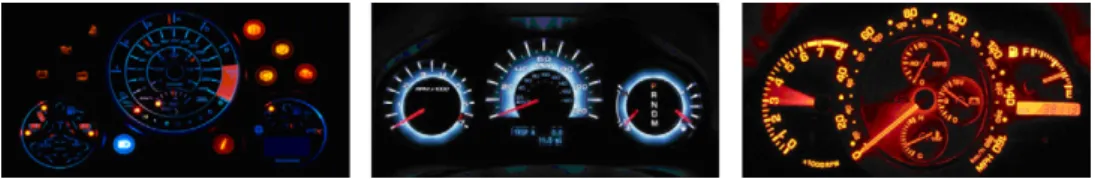
These modern ICs, besides being an essential electronic interface with the user (Wei, Xian-Kui, Lei, Rui, & Bin, 2006), also represent a strong stylish element to the consumer. They have a great influence in the internal aspect of the vehicle, and transmit different kinds of sensations to the user, such as modernity, sport-iveness, futurism, classic,etc. (seeFig. 1). However, in addition to
the attractive graphic design of the ICs, it is essential that they present an appropriate visual quality.
Visual quality is a highly subjective concept that depends on the user’s perception, but it is also influenced by photometric features such as color (i.e., saturation and hue combination) and intensity. In this work, we consider that the visual quality of an IC is determined by a uniform distribution of the light intensity. Visual systems like ICs can present several problems regarding light intensity, which can cause visual discomfort to the vehicle user.
Fig. 2illustrates some of these problems. As observed, inFig. 2(a)
the light intensity concentrates in the middle of the ideogram, while in Fig. 2(b) some regions are brighter or darker than the others. InFig. 2(c) the light intensity is higher on one side or corner than the others.
Aiming to avoid these problems with light intensity, manufac-tures usually employ a validation methodology to assess the visual quality of the components of an IC. Most of the current methodol-ogies used in industry are based on human visual inspection, which is highly subjective, or semiautomatic methods. An example of a semiautomatic method is the use of a spectrophotometer,i.e., an expensive and specialized equipment used to measure light inten-sity. The main problem in the use of a spectrophotometer is that its measurements are very time-consuming. For instance, the valida-tion of a vehicle IC, which usually contains in average 400 possible
0957-4174/$ - see front matterÓ2011 Elsevier Ltd. All rights reserved. doi:10.1016/j.eswa.2011.09.126
⇑Corresponding authors. Addresses: Universidade Federal de Minas Gerais, Computer Science Department, Belo Horizonte-MG, Brazil (A.W.C. Faria), Univer-sidade Federal de Ouro Preto, Computing Department, Ouro Preto-MG, Brazil. Fax: +55 31 3559 1692 (D. Menotti).
E-mail addresses: [email protected](A.W.C. Faria), [email protected]
(D. Menotti),[email protected](G.L. Pappa),[email protected](D.S.D. Lara),
[email protected](A. de A. Araújo).
Contents lists available atSciVerse ScienceDirect
Expert Systems with Applications
measurement points, can take almost 3 h of work. In addition, this type of analysis does not include any scientific criterion for deter-mining acceptable intensity homogeneity levels based on human perception.
In this direction, the first attempts to introduce human percep-tion into the validapercep-tion process of visual interactive systems was concerned with the automatic identification ofMuraon monitors and displays using images analysis (Lee & Yoo, 2004; Oh, Yun, &
Park, 2007).Murais a Japanese word that describes a non-uniform
variation in the local intensity of a region that does not present a
defined contour, and it is noticeable as a visual unpleasant sensation.
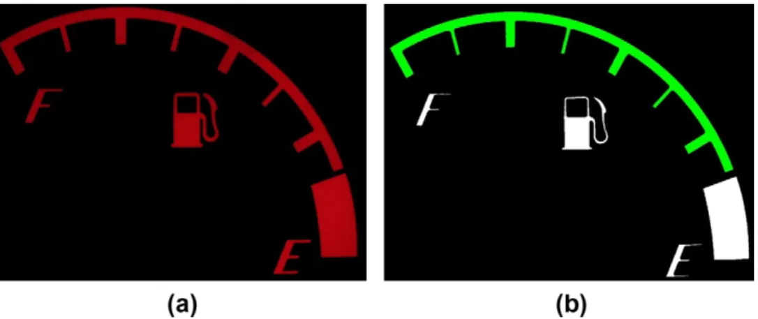
Although the methodologies proposed so far are suitable for validating a unique region (surface), they are not recommended for problems as the one tackled in this work. This is because an IC represents a set of basic instruments (or components – see Fig. 3(a)), such as the speedometer, the fuel and temperature gauges, or the tachometer. Each component is formed by a set of connected regions (seeFig. 3(b)), which can be segmented and la-beled, as shown inFig. 3(c). Hence, we need a methodology that Fig. 2.Typical problems of intensity homogeneity in visual interactive systems: (a) light intensity concentrated in the middle of the ideogram, (b) some numbers are brighter than others, and some regions are very dark, (c) light intensity is higher in the left than in the right side.
considers both the (local) brightness homogeneity in a single com-ponent region, as well as the impact that each small region has in the global visualization of the component.
In this direction, the main goal of this work is to develop a meth-odology based on both digital image analysis and the human visual perception (user’s evaluation) to validate the instruments of an IC. By validate we mean to evaluate if a component presents a good, a critical or a poor visual quality to the user. Note that this work fo-cuses on a single component of the IC (e.g., the speedometer) instead of a set of components,i.e., the IC. The latter is left for future work.
The proposed methodology preprocesses and extracts intensity homogeneity descriptors from a set of acquired component images. At the same time, users evaluate the components and iden-tify their non-homogeneous regions. The users perceptions are then combined with the intensity homogeneity descriptors, and la-ter given to two machine learning algorithms, namely Artificial Neural Network (ANN) and Support Vector Machine (SVM). These algorithms learn to identify homogenous and non-homogenous re-gions and, given a new component image, validate it as a good, crit-ical or poor visual quality.
A preliminary version of this work appears inFaria, Menotti, Lara, Pappa, and Araújo (2010), where the methodology was first introduced. However, inFaria et al. (2010), a single dataset ob-tained from the classification of a specialist was given as input to two machine learning algorithms. Here, we extend the set of experiments so that six different datasets are used. These datasets were created based on the opinions of five ordinary drivers regard-ing the ICs. The analysis performed by the users is contrasted with the analysis of the specialist, as well as the results obtained by the machine learning algorithms with these datasets. Moreover, an overview of the automotive systems of visual interaction is given, and some formalisms are introduced to better describe the pro-posed methodology.
By identifying the non-homogeneous regions of the instru-ments, we will contribute in an effective way to the industrial development process of IC, reducing significantly the time of qual-ity analysis.
The remainder of this work is organized as follows. Section2 introduces basic concepts regarding lighting systems. Section 3 presents the proposed methodology. An analysis of the users’ and specialist’s evaluations is performed in Section 4. Section 5 pre-sents the experiments performed to validate the proposed method-ology. Finally, conclusions and future works are pointed out in Section6.
2. Automotive systems of visual interaction
This section introduces some basic concepts of visual ergonom-ics necessary to understand the users analysis. According to the International Ergonomics Association (IEA), ergonomics is the sci-entific discipline that studies the interactions between men and the environment where they live in, and its main objective it to im-prove men’s welfare and their interaction with the environment.
In the automotive environment, the visual ergonomics regards the harmony of the illumination of IC, considering colors, contrast, reflexes, ghost lights, lighting distribution (homogeneity), glare,
etc. Its main objectives are to improve the safety and comfort of the human visual system, avoiding fatigue.
As indicated byWalraven et al. (2001), the visual ergonomics of aircrafts interaction systems, which is extensible to the automotive industry, comprehends two types of evaluation:
Cognitive: Studies the efficiency of the information transmis-sion by the instruments, which should be easily readable, of fast interpretation, and not give margins to double meanings.
Visual quality of the instrument: Studies the color, intensity and homogeneity of the luminous distribution of the component.
In this work, we focus on the visual quality of the instrument, studying the perception that users have on the illumination homo-geneity of the components.
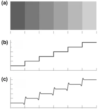
In this context,Gonzalez and Woods (2007)describe two inter-esting effects in the human perception of the lighting intensity that an object has in relation to its context. The first effect, exemplified by the Mach1bands, shows that the perception of the lighting inten-sity is not only given in function of the object. The human visual sys-tem tends to exceed or to reduce the intensity perception as it approximates or stands back from another level of intensity. For example, inFig. 4(a), although the intensity of each column is con-stant, the intensity perception of the transition regions are brighter for dark columns and darker for bright columns.Fig. 4(b) and (c) highlight this effect.
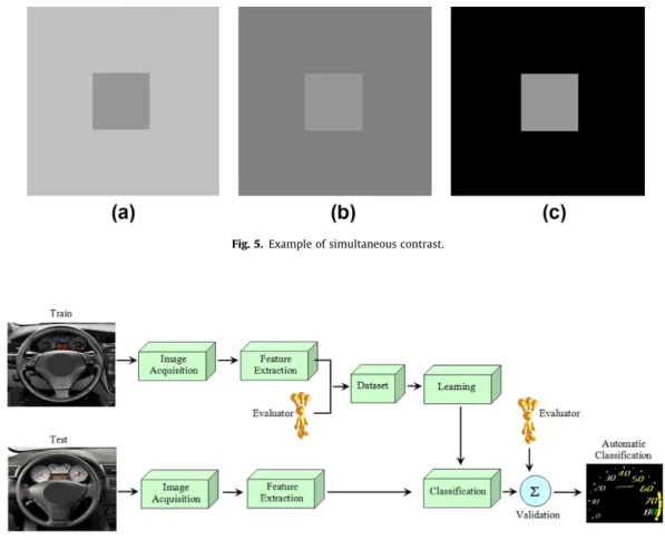
The second effect, called simultaneous contrast, also shows that the perception of the intensity is strongly influenced by the back-ground in which the object is inserted. For instance, in Fig. 5, although the central square (object) has the same intensity in the three images, as soon as the background becomes darker the hu-man perception tends to notice the object brighter.
Regarding studies considering the ergonomics of automotive interactive systems, they first appeared right after the Second World War, where several components (gauges) were added to the aircrafts cockpits. The equipments were designed to give valu-able information to the pilots, but their interface did not allow pi-lots to make a correct and fast interpretation of their readings. This was mainly because of the lack of good visibility of some instru-ments and the non-standardization of the instruinstru-ments disposition in the cockpit. As a consequence, countless accidents happened, and from then many studies were performed to modify the original projects to improve the operability and visualization for the pilot. Fig. 4.Mach bands effect: (a) growing levels of intensity; (b) real intensity; (c) noticed intensity.
Contemporaneously to the studies of the ergonomics applied to aviation appeared the studies in the automotive industry. Their main goal was to provide drivers a comfortable and easy interac-tion environment. In this scenario, the IC became the main channel of interaction between the driver and the car. Along the years the IC has become one of the most complex embedded electronic systems in modern vehicles (Huang et al., 2008), providing the dri-ver with a didri-verse unidri-verse of information, from drive conditions, messages and pre-diagnostics to multimedia systems (Castineira et al., 2009).
3. Methodology
This section describes the methodology proposed to identify, in an automatic way, regions with non-homogeneous lighting on components using image analysis.Fig. 6shows a general scheme of the proposed methodology for the automatic validation of the internal lighting system of an automobile.
In the first step, the images are acquired using a meticulous pro-cedure that guarantees the image reflects in the best possible way the real lighting condition. This process is described in detail in Section3.1. The image acquisition is followed by a feature extrac-tion phase, described in Secextrac-tion3.2, where a set of features (or descriptors) that reflect the lighting distribution in the image are calculated. Here a new descriptor, which takes into account the global light intensity, is proposed.
These set of features extracted from the images are then associ-ated with a set of labels given to the regions of the images by the users, generating datasets. These datasets are then given to two classification algorithms: Support Vector Machine (SVM) and Arti-ficial Neural Network (ANN), as detailed in Section3.4, which will automatically classify component regions as being homogenous or
not. Finally, based on the number of regions classified as non-homogenous, a component is classified as acceptable, unacceptable or in need of attention.
Note that the evaluation of the components performed by the users is the most difficult and subjective part of this process. Hence, we leave to discuss it with a high level of details in Section4.
3.1. Image acquisition
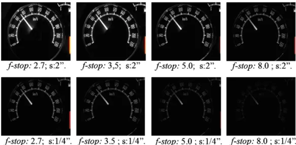
The methodology proposed in this work is highly dependent on the quality of the acquired images. As we are analyzing the images according to their light intensity, we need them to reproduce as faithfully as possible the patterns of light distribution of a compo-nent. In photography, parameters such as the Shutter Speed (s) and the Diaphragm Opening (f-stop) have great influence in the image exposure (Gimena, 2004).Fig. 7shows the effects of varying these parameters for image acquisition.
In order to obtain the best parameter values forsandf-stop, we selected two IC components of different colors and used a spectro-photometer to measure their ‘‘real’’ light intensities in a set of 52 points, as showed inFig. 8. We chose to use the spectrophotometer due to its very accurate measurements. After that, we acquired images for these two IC components using a basic digital camera with sixsvariations (1/500; 1/800; 1/1000; 1/1300; 1/1500, and 1/2000),
letting thef-stopfixed to 2.7. We chose a small value forf-stop be-cause the depth of field2(Peterson, 2004) should be as shallow as possible, since we want to focus only on the IC. Thef-stopwas fixed because there is a reciprocity law between shutter speed and diaphragm opening,i.e.,sandf-stophold a direct relation (Gimena, Fig. 5.Example of simultaneous contrast.
Fig. 6.A diagram of the proposed methodology.
2004).
Having the set of acquired images, we selected for each of them the pixel values corresponding to each of the 52 points previously measured by the spectrophotometer in the ‘‘real’’ IC component
(seeFig. 8). The pixel values of the image were taken from the V
(value/intensity) channel of the HSV color system (Gonzalez & Woods, 2007). We wanted to compare the values measured by the spectrophotometer with the ones found in the images. In order to do that, we first normalized both values following the max–min rule (Martinez, Sanches, Prados, & Pereles, 2005),i.e.,
z¼maxxminðxÞ
ðxÞ minðxÞ; ð1Þ
wherexrepresents the pixel value.
The values obtained are shown inFig. 9. From these normalized values, we calculated the Mean Square Error (MSE) between the spectrophotometer reading and the corresponding pixel value in the image,i.e.,
MSE¼1 n
X
n
i¼1
ðxixÞ
2
; ð2Þ
wherenis the number of points,xis the value read by the spectro-photometer, andxiis the pixel value in pointi.
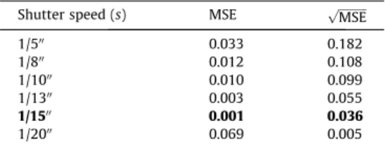
The results obtained are reported inTable 1. The figures inTable 1show that the camera setup that best represents the measure-ment done by the spectrophotometer is the one with shutter speed
s= 1/1500. Therefore, all images used in this work were acquired
with a digital camera withf-stop= 2.7 ands= 1/1500.
3.2. Feature extraction
After acquiring the images, the methodology for IC components validation proposed in this work preprocesses and extracts inten-sity homogeneity descriptors from these images.
As previously explained, each IC component is represented by several connected regions. The image preprocessing step has as its main goal to identify these regions. Hence, the original image is submitted to the following procedures, as illustrated inFig. 10:
Image conversion from RGB (Red, Green and Blue) to HSV (Hue, Saturation and Value) color space. The HSV color space was cho-sen because it reprecho-sents the colors in a more intuitive manner. The V channel (Value/Intensity/Brightness) is taken as the light-ing intensity representative (Gonzalez & Woods, 2007).
Image thresholding (Otsu, 1979). This process sets pixel values above some threshold to 1 (white) and below this threshold to 0 (black).
Image erosion (Serra, 1984). Erosion is a morphologic operation used to eliminate irrelevant details from an object, starting from pixels in the borders. The reason for using erosion in this work was to eliminate undesirable border pixels that appeared due to camera resolution.
Labeling of connected components (Shapiro & Stockman, 2002). Labeling is an effective technique for binary image segmenta-tion. It examines the connectivity of the pixels with their neigh-bors and labels connected sets. This method was used to extract and identify the regions present in a component.
3.3. Homogeneity descriptors
After identifying the regions of an image, we extract a set of descriptors that represent the light homogeneity in each region of the component. Our goal is to later associate these descriptors with a category defined by the user. This category says whether the region is homogenous or not according to the user’s sensations. Fig. 7.Differences obtained in the images when calibrating thef-stopand shutter speed (s) parameters.
Several metrics have already been proposed in the literature to compute the light homogeneity of a region (Cheng & Sun, 2000;
Gimena, 2004). InOh et al. (2007), for example, the authors define
the Lighting Uniformity metric,i.e.,
ULðRÞ ¼ ðrmin=rmaxÞ 100; ð3Þ
wherermaxandrminrepresent the maximum and minimum
inten-sity values of a region R, respectively. In Gonzalez and Woods (2007) and Borges, Mayer, and Izquierdo (2008), the intensity distri-bution is defined by statistical moments of the levels of the histo-gram of a region. Let R be a random variable denoting levels of the regions and letPR(ri),i= 0, 1, 2,. . .,L1, be the corresponding
histogram, whereLis the number of distinct levels. Then, thenth moment ofRis defined as:
l
nðRÞ ¼X
L1
i¼0
ðrimðRÞÞ n
PRðriÞ; ð4Þ
where
mðRÞ ¼X
L1
i¼0
ðriPRðriÞ; ð5Þ
wheremstands for the average level. From these equations, other statistical moments, namely the 3rd moment (Eq.(6)), uniformity Fig. 9.Calibrating the digital camera – normalized values: spectrophotometer measurementsversuspixel reading values.
Table 1
Mean square error between the spectrophotometer readings and its corresponding pixel values in the image. The camera setup with 1/1500value for shutter speed is the one that best represents the measurement done by the spectrophotometer.
Shutter speed (s) MSE ffiffiffiffiffiffiffiffiffiffi MSE p
1/500 0.033 0.182
1/800 0.012 0.108
1/1000 0.010 0.099
1/1300 0.003 0.055
1/1500 0.001 0.036
1/2000 0.069 0.005
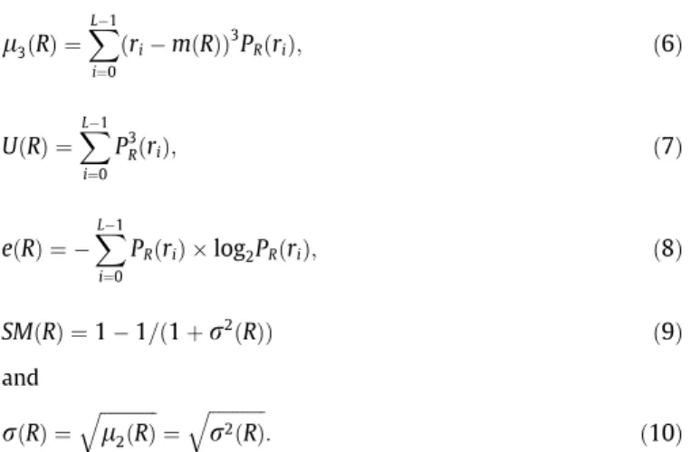
(Eq.(7)), entropy (Eq.(8)), smoothness (Eq.(9)), and standard devi-ation (Eq.(10)) can be estimated as
l
3ðRÞ ¼X
L1
i¼0
ðrimðRÞÞ
3
PRðriÞ; ð6Þ
UðRÞ ¼X L1
i¼0
P3RðriÞ; ð7Þ
eðRÞ ¼ X
L1
i¼0
PRðriÞ log2PRðriÞ; ð8Þ
SMðRÞ ¼11=ð1þ
r
2ðRÞÞ ð9Þand
r
ðRÞ ¼ffiffiffiffiffiffiffiffiffiffiffiffi
l
2ðRÞq
¼ ffiffiffiffiffiffiffiffiffiffiffiffi
r
2ðRÞq
: ð10Þ
The descriptors presented in Eqs. (3) and (6)–(10) were ex-tracted from each of the component regions. Furthermore, we are also interested in the impact each region has in the global unifor-mity (GU) of the entire component. Hence, we propose a descriptor that considers both the local region and global component intensi-ties, named as Relative Descriptor (Faria et al., 2010) and defined as
RDðRÞ ¼ ðmLðRÞ=mGÞ 100; ð11Þ
wheremL(R) andmGstand for the average intensity of a regionR
and the average intensity of the whole component (or instrument) in analysis, respectively.
These descriptors were associated with the labels given by the user through the process detailed in Section4, and given to the ma-chine learning algorithms described in the next section.
3.4. Machine learning
Machine learning refers to a set of methods that can learn from data (Duda, Hart, & Stork, 2000; Mitchell, 1997). Given a set of examples, described by a set of attributes (descriptors), machine learning algorithms can perform three types of learning: super-vised, semi-supervised and unsupervised. In this work, the learner will deal with supervised learning, as the categories the examples belong to (homogeneous or not) are known. The learner works by finding relationships between the attributes that describe an example and the category it is associated with.
There are many types of machine learning algorithms that could be used to solve the problem tackled in this paper. We chose to use two state-of-the-art classification algorithms: Support Vector Machine (SVM) and Artificial Neural Network (ANN).
Support Vector Machines (SVMs) (Scholkopf & Smola, 2002) are methods that build classifiers by constructing hyper-planes in an -dimensional space, i.e., by drawing ‘‘lines’’ in the n-dimensional space that are able to separate examples from different classes. When faced with non-linear problems, SVMs create a mapping be-tween a set of input values (examples) and a feature space, where these initially non-linear class boundaries are made linearly sepa-rable via a transformation (or mapping) of the feature space. This mapping is done by a set of mathematical functions called kernels. After performing this mapping, SVMs use an iterative training algo-rithm to minimize an error function.
Artificial Neural Networks (ANNs) (Bishop, 1996) are computa-tional systems inspired by the way the nervous system and the hu-man brain process information. They have become popular due to their capabilities to deal with irregularities, work with uncertain, incomplete and/or insufficient data, and have proved to be power-ful tools to find patterns in data, including non-linear relationships.
4. User’s evaluation of instruments
As explained before, the homogeneity descriptors extracted from each region should be associated with a category,i.e., homog-enous or not. This characterization will allow us to, in a next step, automatically identify non-homogeneous regions in a component in analysis, taking into account human perception.
Hence, 48 common drivers and one automotive lighting special-ist were chosen to perform the analysis of the components. The experiment with common drivers involved 35 men and 13 women, with ages from 20 to 50 years, having height varying from 1.55 m to 1.90 m, different professional activities, some using vision cor-rective systems (lenses and glasses) and others not. The variety of the group provides a representative sample of common drivers. Every IC component, from a set of 107 IC components, obtained from 30 ICs, were evaluated by five different users and the special-ist. The components were distributed for the users in a way that any two users would not evaluate more than one common instru-ment. The specialist evaluated all the instruments, generating a gold-standard dataset for comparisons.
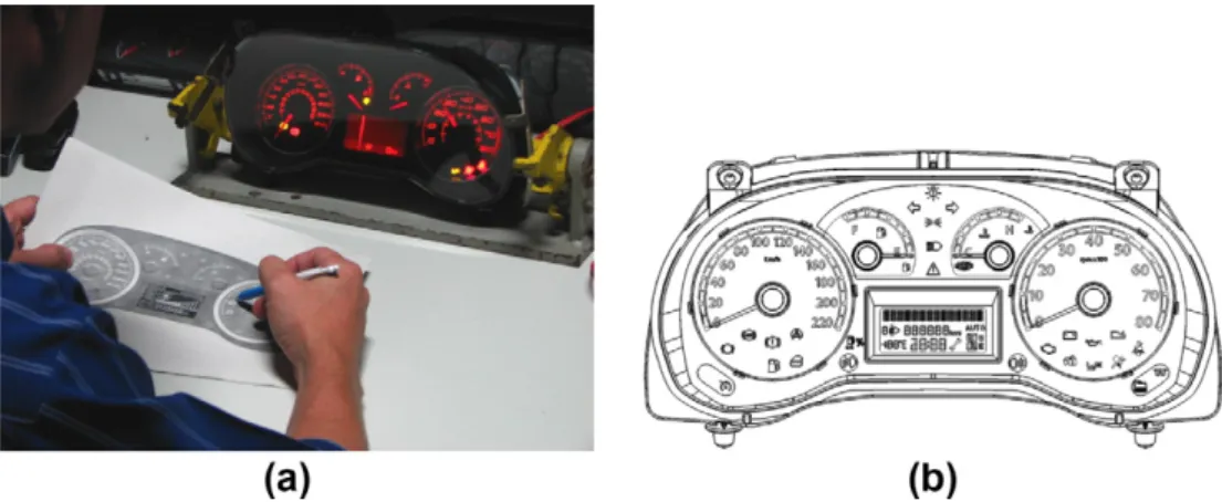
The instruction given to each evaluator was: ‘‘identify regions of the IC components that present lack of homogeneity’’. All the eval-uations were performed in a dark chamber, with all environment lights off, emulating a real driving condition at night. The IC was fixed in a bench test (seeFig. 11(a)), respecting the position and average inclination it would have in a vehicle in relation to the dri-ver. For each IC, a schematic drawing was given to the user (Fig. 11(b)), who marked in this drawing the regions where they judged there was ‘‘lack’’ of homogeneity.
At the end of the evaluation procedure, we noticed there was a high level of disagreement among users when identifying non-homogenous regions. This result highlights the subjectivity and difficulty of the problem. In order to label groups of non-homoge-nous regions, we decided to set an agreement threshold, based on the number of users that identified a region as non-homogenous. Note that this part of the process does not take into account the opinion of the specialist, only the common users. We chose to cre-ate five different datasets according to this agreement threshold. A datasetn is composed by all regions classified as non-homoge-neous by at leastnusers. Hence, Dataset 1 has all regions classified as homogenous by any user, and it is the set with more non-homogenous samples (seeTable 2), Dataset 5, in contrast, has only 0.65% of non-homogenous regions, as it requires that all five users agree the region is non-homogenous.
Table 2presents the distribution of classes (non-homogeneous
(NH)/homogeneous (H)) for each dataset based on the agreement threshold and the specialist. The data are expressed in percentage and absolute numbers. Note that Dataset 2 presents a class distri-bution similar to that generated by the specialist.
4.1. Contrasting common users and specialist evaluations
This section contrasts the opinion of the users among themselves and with the opinion of the specialist when classifying homogenous and non-homogenous regions. The degree of agreement regarding non-homogeneous or homogeneous regions (represented byXin Eq.(12)) is defined as
AgreementðX;D1;D2Þ ¼
#ðD1ðXÞTD2ðXÞÞ
#ðD1ðXÞSD2ðXÞÞ; ð
12Þ
where Dn(X) represents the set of regions of type X (i.e.,
Tables 3 and 4 present the degree of agreement among each dataset pair. An agreement of 1 says that all the labels are the same for the two groups (or datasets). As expected, the figures in the ta-bles show that there is a higher level of agreement for homoge-neous labeling than non-homogehomoge-neous. This is natural as the images tend to present much more homogenous regions (and these ones can be easily identified by the user). Considering non-homo-geneous regions, the opinions vary a lot according to the users sen-sitivity to the lightning system (some are more critical and others more tolerant). We also note that the largest number of
disagree-ments occurs in regions close to the global perception threshold between homogeneous and non-homogeneous, which varied from user to user.
Considering the agreements among the specialist and the five datasets generated by the users’ evaluations, again in the homoge-neous regions the agreement indexes are relatively high, reaching 0.81. However, for the non-homogeneous regions, they did not go over 0.33.
4.2. Users opinions on the specialist evaluation
In this work, we assume the knowledge and experience of the specialist makes it easier for him to identify non-homogenous re-gions correctly. However, it is important for us to know if the com-mon users agree with the specialist evaluations. Hence, in order to find out if the specialist evaluation really represents the general users’ perception, a new experiment was performed, and the users evaluated the classifications made by the specialist.
Each user received a schematic drawing were all the non-homogenous regions identified by the specialist, and that the industry assumes needs correction, were marked. They were taken to the bench test in a darkroom, and were asked the following question: ‘‘how do you evaluate the suggested corrections (the specialist’s evaluation)?’’. The user had three options, in a scale from 1 to 3:
1. Inadequate: After correcting the suggested regions the instru-ment would not present a homogeneous illumination. 2. Appropriate: After correcting the suggested regions the
instru-ment would present a suitable illumination.
3. Excessive: It is not necessary to correct all regions for the instru-ment to present a good illumination.
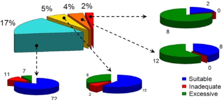
Each instrument was evaluated by 5 different users and each user evaluated 10 instruments on average. In total, 535 evaluations (5 users107 IC components) were performed. The graph in
Fig. 12summarizes the results obtained after evaluation.
Analyzing the graph, we observe that 72% of the specialist’s labeling were considered by 5 out of 5 users as appropriate, while 17% were considered appropriate by 4 out of 5 users. The remain-ing 11% are evaluations where only one, two or three users found the change appropriate. From the 535 evaluations, only 48 were considered as not appropriate by the users, obtained an acceptance rate of 91% on the specialist labeling.
Fig. 13shows in more detail the opinions of users when they
dis-agree with the specialist correction. From the 48 labeled evalua-tions considered as not appropriate, 73% were classified as excessive, and only 27% as insufficient. It is important to point Fig. 11.The evaluation setup: (a) the IC; (b) the drawing given to the user.
Table 2
Distribution of homogeneous (H) and non-homogenous (NH) regions for each of the 6 datasets generated. In total, 3410 regions were extracted from 107 IC components.
Evaluator Regions
NH (%) H (%) NH (#) H (#)
Dataset 1 41.32 58.68 1409 2001
Dataset 2 20.56 79.44 701 2709
Dataset 3 8.83 91.17 301 3109
Dataset 4 3.43 96.57 117 3293
Dataset 5 0.65 99.35 22 3388
Specialist 20.59 79.41 702 2708
Table 3
Agreement matrix for non-homogeneous regions.
Dataset 1
Dataset 2
Dataset 3
Dataset 4
Dataset 5
Specialist
Dataset 1 1.00 0.50 0.21 0.08 0.02 0.32
Dataset 2 0.50 1.00 0.43 0.17 0.03 0.33
Dataset 3 0.21 0.43 1.00 0.39 0.07 0.22
Dataset 4 0.08 0.17 0.39 1.00 0.19 0.12
Dataset 5 0.02 0.03 0.07 0.19 1.00 0.02
Specialist 0.32 0.33 0.22 0.12 0.02 1.00
Table 4
Agreement matrix for homogeneous regions.
Dataset 1
Dataset 2
Dataset 3
Dataset 4
Dataset 5
Specialist
Dataset 1 1.00 0.74 0.64 0.61 0.59 0.63
Dataset 2 0.74 1.00 0.87 0.82 0.80 0.77
Dataset 3 0.64 0.87 1.00 0.94 0.92 0.80
Dataset 4 0.61 0.82 0.94 1.00 0.97 0.81
Dataset 5 0.59 0.80 0.92 0.97 1.00 0.80
out that there was no correction considered as not appropriate by all 5 users.
5. Computational results
Having created the datasets, experiments were performed in two phases. First the regions of the images are classified as homog-enous or not by the machine learning algorithms. Then, based on the number of non-homogenous regions, the instruments are clas-sified as acceptable, unacceptable or in need of attention.
Throughout this section, the results obtained by the machine learning algorithms are presented in the form of confusion matri-ces. The values in these matrices are presented in percentage ((#). Those express the average and the standard deviation (
l
±r
) of 107 tests performed through leave-N-out/leave-one-outvalidation, where N stands for the number of regions of each instrument when an instrument is left out (i.e., leave-one-out). Note that the high values of standard deviation in the confusion matrices are due to the great variation in the number of regions found in each instrument. For instance, some fuel gauges have 7 re-gions, while some speedometers have 80 regions.
5.1. Classifying instrument cluster regions
This section shows the classification of the instrument regions. As previously mentioned, we worked with ANN and SVM, using MatLab implementations. As we are dealing with non-linear data, the standard Matlab SVM algorithm was modified to use a
polyno-mial kernel function of order 3. The ANN chosen is the Multi-Layer Perceptron (MLP) feed-forward back propagation, trained with a Levenberg Marquardt function. The network architecture was set-up with one hidden layer, with a number of neurons equals to 2/3 of the neurons in the input layer. All the neurons used the inverse transcendental tangent function as an activation function. The training stop criterion was a MSE smaller than 102, or 500 epochs.
Table 5presents a summary of the general accuracy of the
mod-els trained and tested with the ANN and SVM. InTable 5, we ob-serve that the evaluation performed by the specialist and the users with agreement threshold 4 and 5 obtained the best results for the general classification of the regions. However, note that the classification of datasets 4 and 5 were expected to be good, as they have really unbalanced classes. Predicting all classes as homogenous would lead to accuracies of 96.57% and 99.35%, respectively. Hence, the accuracy is not a good measure to evaluate the results.
Table 6shows results of precision per class. Note that, in this
case, the data labeled by the specialist is the one where the classi-fiers better learn to distinguish the classes, with precisions around 94% for non-homogenous and 97% for homogenous regions. In this scenario, Dataset 4 predicts 2.38% of regions correctly while Data-set 5 does not provide enough information for learning. From these experiments, we conclude that the specialist labeling was the best for learning followed by Dataset 1. In any case, while the specialist obtained 95% accuracy for NH regions, Dataset 1 obtained 53%.
Recall that Dataset 1 requires a single user to classify a region as non-homogeneous while in Dataset 5 all five evaluators have to be under agreement. Thus, the number of non-homogeneous regions Fig. 12.Summary graph of the users opinion on the specialist evaluation.
in Dataset 5 is smaller than in Dataset 1. The analysis performed here can be well understood by the confusion matrix of this exper-iment, shown inTable 7.
5.2. Classifying instrument cluster components
The previous section presented the results obtained when clas-sifying IC component regions. However, our aim is to classify a whole component (instrument) based on the classification of its re-gions. We propose to classify components into three categories, which depend on the number of classified non-homogenous re-gions. Each category is described as follows:
Accept: The instrument presents less than or equal to 5% of its regions classified as non-homogeneous.
Attention: The instrument presents more than 5% and less than or equal to 10% of its regions classified as non-homogeneous, and the manufacturer should take that into account in the project.
Reject: The instrument presents more than 10% of its regions classified as non-homogeneous.
In this case, the manufacturer should modify the project of the IC.
The 5% and 10% tolerance levels are based on the practical expe-rience of the specialist.Table 8shows the class distribution of the instruments according to this classification. As observed, the class distribution varies a lot from one Dataset to another. For instance, Dataset 5 rejects only 1 IC, while the Specialist rejects 57. The re-sults obtained are shown inTables 9 and 10.
A summary of all these results is shown inTable 10, which re-ports the precision for the IC component classification, as well as the number of what we call critical errors,i.e., the acceptation of a bad IC component. Here, classifying a bad IC component as a good one is much more serious than the opposite, as after product accep-tation it is used as a ‘‘model’’ for the whole product chain process.
Analyzing the results generated when using the specialist’s labeling inTable 9, we note that there were only 6 (resp. 7) out of 107 wrong classifications for the ANN (resp. SVM), none of them considered critic. Analyzing the results generated by the datasets based on users’ evaluations, we note that in average the precision is smaller than that obtained by the specialist’s evaluation, and the number of critical errors varies from 11 to 30 for the first four data-sets, being Dataset 3 the most critical one. The precision obtained by the users’ labeling in Dataset 5 is as high as those made by the specialist, and the classification resulting from this labeling pre-sents just one critical mistake. The same types of results are ob-tained by the ANN (resp. SVM), with 11 (resp. 6) out of 107 wrong classifications, including a critical error. These results can be explained by the low number of NH regions in the Dataset 5 (only 22), as this group requires all users to agree on their evalua-tion. This rarely occurs in practice due to the subjectivity of the evaluation process.
5.3. Visualization of IC components classifications
This section presents and discusses the classification of four IC components images classified by the system. Each column in Table 6
Precision values per class.
Evaluation Non-homogeneous Homogeneous
ANN (%) SVM (%) ANN (%) SVM (%)
Dataset 1 53.68 40.19 82.39 86.97
Dataset 2 34.65 22.12 94.42 96.63
Dataset 3 9.37 5.20 98.20 99.23
Dataset 4 2.38 0.00 99.42 99.93
Dataset 5 0.00 0.00 98.58 99.42
Specialist 94.79 93.01 97.75 97.34
Table 7
Confusion matrix: classification for the regions.
l%(r%) Observed
ANN SVM
NH (%) H (%) NH (%) H (%)
Expected NH Group 1 19.02(18.55) 16.41(14.58) 14.24(15.27) 21.19(16.68)
Group 2 6.05(7.89) 11.41(13.13) 3.86(5.86) 13.59(14.44)
Group 3 0.74(2.24) 7.15(9.44) 0.41(1.18) 7.47(9.41)
Group 4 0.07(0.49) 2.86(4.66) 0.00(0.00) 2.94(4.79)
Group 5 0.00(0.00) 0.58(1.71) 0.00(0.00) 0.58(1.71)
Specialist 15.47(15.89) 0.85(1.87) 15.17(15.58) 1.14(2.37)
H Group 1 11.37(11.37) 53.20(27.58) 8.41(10.48) 56.16(27.49)
Group 2 4.75(7.82) 77.79(19.71) 2.78(5.18) 79.76(18.73)
Group 3 1.65(5.30) 90.47(11.50) 0.71(1.83) 91.41(10.29)
Group 4 0.56(2.71) 96.50(5.52) 0.06(0.60) 97.00(4.79)
Group 5 1.41(7.45) 98.01(7.54) 0.00(0.00) 99.42(1.71)
Fig. 14represents an image. In the first row are the original images, followed by the resulting images of the classification based on the specialist, Dataset 1 and Dataset 5, respectively. For these last images the classification generated by the system is represented by colors. The homogeneous and non-homogeneous regions cor-rectly classified appear in white and yellow, respectively. The non-homogeneous regions classified as homogeneous (critical er-rors) are in red, whilst the homogeneous regions classified as non-homogeneous appear in green.
Observing the images inFig. 14, we verify that in Dataset 1 great part of the regions are considered as non-homogeneous. On the other hand, in Dataset 5 almost 100% of the regions are accepted as homogeneous. Analyzing these images, some facts previously verified by the computational experiments can be confirmed. The results obtained by the specialist’s labeling (second line) show very few regions misclassified, which did not impact the final classifica-tion of the instrument (accept or reject). The results obtained by Dataset 1 (third line) present a lot of regions erroneously classified, directly contributing to the final misclassification of the instru-ment. Dataset 5 has the problem of highly unbalanced classes, which makes that the few non-homogeneous regions are wrongly classified as homogeneous.
As claimed in the last subsection and shown inTable 10, the proposed methodology achieve promising results by using the spe-cialist for training the classifiers. In the following, we illustrate an example where the classification using the specialist labeling makes a mistake but not a critical one.
Fig. 15(a) presents an image of an instrument and its respective classification based on the specialist’s labeling (Fig. 15(b)), which
had a wrong final classification. All the regions of this image were originally labeled as homogeneous by the specialist. However, in the classification performed by the methodology using all the other specialist’s labelings, the region at the top of the image (that one marked on green) is classified as non-homogeneous. As the num-ber of the classified non-homogeneous regions in the instrument is greater than 5% of the total number of regions, its final classifi-cation is considered as rejected. In that situation there is a mistake in the final classification of the instrument, which should be ac-cepted. However, this error is not considered a critical mistake,
i.e., accepting a ‘‘bad’’ instrument.
5.4. Final considerations
The methodology proposed in this work has proved to be effec-tive in automatically identifying non-homogeneous regions in a component from an instrument cluster, used to aid the classifica-tion of the complete instrument as accepted, on need of attenclassifica-tion, and rejected. The two classifiers used in this work (ANN and SVM) obtained similar results for both the users’ evaluation and the spe-cialist’s evaluation. An analysis on the number of descriptors used in the models learnt showed that SVM uses less descriptors than the ANN, achieving equivalent results in terms of precision.
The evaluations were divided in two groups:
1. Labeling with the specialist: Appropriate learning of the algo-rithms; not so unbalanced distribution of the classes (homoge-neous and non-homoge(homoge-neous) and high precision in the final classification of the instrument (acceptedversus rejected). 2.Labeling with the users: Deficient learning of the algorithms;
quite unbalanced distribution of the classes (biased learning on the homogeneous class) and final classification of the instrument with critical mistakes (acceptation of ‘‘bad’’ instruments, i.e., instrument with more than 5% of non-homogeneous regions).
The specialist’s technical evaluation provided a learning for the classifiers which generates the best precision for both non-homo-geneous and homonon-homo-geneous classes. Through the users’ evaluations about the specialist’s evaluation, it was possible to notice that the specialist represents the average perception of users very well, obtaining an index of acceptance higher than 90%.
Table 9
Confusion matrix: final classification for the instruments.
Observed
ANN SVM
Accepted Attention Rejected Accepted Attention Rejected
Expected Accepted Dataset 1 6 2 6 7 3 4
Dataset 2 36 2 3 39 1 1
Dataset 3 57 0 1 58 0 0
Dataset 4 77 1 2 79 1 0
Dataset 5 97 1 4 101 0 0
Specialist 42 1 4 41 2 4
Attention Dataset 1 4 0 2 4 1 1
Dataset 2 2 0 3 2 1 2
Dataset 3 3 3 2 4 2 0
Dataset 4 15 0 0 15 0 0
Dataset 5 5 0 0 5 0 0
Specialist 0 2 1 0 2 1
Rejected Dataset 1 18 2 67 22 6 59
Dataset 2 12 7 42 18 10 33
Dataset 3 30 8 5 38 4 1
Dataset 4 11 0 1 12 0 0
Dataset 5 1 0 0 1 0 0
Specialist 0 0 57 0 0 56
Table 10
Summary of the accuracy of the classification of the instrument.
Evaluation ANN SVM
Precision (%) Critical errors Precision (%) Critical errors
Dataset 1 71.96 18 62.62 22
Dataset 2 72.89 12 68.22 18
Dataset 3 60.75 30 57.00 38
Dataset 4 72.90 11 73.82 12
Dataset 5 90.65 1 94.39 1
The proposed methodology presents two main advantages over the method that uses the spectrophotometer: it is cheap to imple-ment (a spectrophotometer is much more expensive than a digital camera) and computationally efficient. These two characteristics
allow the manufacturer of automotive ICs to apply the methodol-ogy in several points of his production line, reducing the number of reproofs made in the assembly line due to instruments with bad illumination.
Fig. 14.Classification of four images according to the generated datasets: homogeneous and non-homogeneous regions correctly classified appear in white and yellow, while misclassified non-homogeneous and homogenous regions are in red and green. (For interpretation of the references to colour in this figure legend, the reader is referred to the web version of this article.)
6. Conclusions
Studies looking to map, characterize, and understand human perceptions are as attractive as complex. Human sensations depend on each individuals experience and acquired knowledge. This work presented a methodology for automatic validation of Automotive Instrument Cluster using the concept of light homoge-neity in images analysis, computational intelligence, and human evaluations. To feed the machine learning algorithms (ANN and SVM), aiming at the classification of the region as homogeneous or not, evaluations were performed by a specialist and ordinary users. The experimental results for classifying both instrument regions and components are above 94%.
The evaluations with the users presented great dispersion among the results. On the other hand, the evaluations accom-plished by the specialist presented good consistence and obtained high acceptance indexes by the users,i.e., more than 90%.
As presented in the introduction, the application of this meth-odology in the industry will help to raise quality and save precious time in the development phase of new instruments. The use of this methodology will also aid the phase of experimental tests in both the assembly line and indicating the manufacturer the points that should be improved in its project.
Acknowledgments
The authors are grateful to CNPq, CAPES and FAPEMIG, Brazilian funding agencies, for the financial support to this work. The first author would like to specially thanks the FIAT Automóveis S/A.
References
Bishop, C. M. (1996). Neural networks for pattern recognition (1st ed.). Oxford University Press.
Borges, P. V. K., Mayer, J., & Izquierdo, E. (2008). Document image processing for paper side communications.IEEE Transactions on Multimedia, 10(7), 1277–1287.
Castineira, F. G., Dieguez, D. C., & Castano, F. J. G. (2009). Integration of nomadic devices with automotive user interfaces. IEEE Transactions on Consumer Electronics, 55(1), 31–34.
Cheng, H. D., & Sun, Y. (2000). A hierarchical approach to color image segmentation using homogeneity.IEEE Transactions on Image Processing, 9(12), 2071–2082. Duda, R. O., Hart, P. E., & Stork, D. G. (2000).Pattern classification(2nd ed.).
Wiley-Interscience.
Faria, A. W. C., Menotti, D., Lara, D. S. D., Pappa, G. L., & Araújo, A. A. (2010). A new methodology for photometric validation in vehicles visual interactive systems. InXXIV ACM symposium on applied computing, track: Computational intelligence and image analysis(pp. 1–6).
Gimena, L. (2004). Exposure value in photography. A graphics concept map proposal. InInternational conference on concept mapping(pp. 256–269). Gonzalez, R. C., & Woods, R. E. (2007).Digital image processing(3rd ed.). Prentice
Hall.
Huang, Y., Mouzakitis, A., McMurran, R., Dhadyalla, G., & Jontes, P. (2008). Design validation testing of vehicle instrument cluster using machine vision and hardware in the loop. InIEEE international conference on vehicular electronics and safety(pp. 22–24).
Lee, J. Y., & Yoo, S. I. (2004). Automatic detection of region-mura defect in tft-lcd. IEICE Transactions on Information and Systems, E87-D(10), 2371–2378. Martinez, J. C., Sanches, D., Prados, B., & Pereles, F. G. (2005). Fuzzy homogeneity
measures for path-based colour image segmentation. In14th IEEE international conference on fuzzy systems(Vol. 5, pp. 218–223).
Mitchell, T. (1997).Machine learning. McGraw Hill.
Oh, J. H., Yun, B. J., & Park, K. H. (2007). The defect detection using human visual system and wavelet transform in tft-lcd image. InFrontiers in the convergence of bioscience and information technologies (FIBIT)(pp. 498–503).
Otsu, N. (1979). A threshold selection method from gray level histograms.IEEE Transactions on Systems, Man and Cybernetics, 9(5), 62–66.
Peterson, B. (2004).Understanding exposure: How to shoot great photographs with a film or digital camera – revised edition. Amphoto Books.
Scholkopf, B., & Smola, A. J. (2002).Learning with kernels: Support vector machines, regularization, optimization, and beyond. The MIT Press.
Serra, J. (1984).Image analysis and mathematical morphology. Academic Press. Shapiro, L., & Stockman, G. (2002).Computer vision. Prentice Hall.
Walraven, J., & Alferdinick, J. W. A. M. (2001).Visual ergonomics of colour-coded cockpit displays: A generic approach(2nd ed.). The Research And Tecnhology Organization (RTO).