www.atmos-chem-phys.net/17/1901/2017/ doi:10.5194/acp-17-1901-2017
© Author(s) 2017. CC Attribution 3.0 License.
Global scale variability of the mineral dust long-wave refractive
index: a new dataset of in situ measurements for climate
modeling and remote sensing
Claudia Di Biagio1, Paola Formenti1, Yves Balkanski2, Lorenzo Caponi1,3, Mathieu Cazaunau1, Edouard Pangui1, Emilie Journet1, Sophie Nowak4, Sandrine Caquineau5, Meinrat O. Andreae6,12, Konrad Kandler7, Thuraya Saeed8, Stuart Piketh9, David Seibert10, Earle Williams11, and Jean-François Doussin1
1Laboratoire Interuniversitaire des Systèmes Atmosphériques (LISA), UMR7583, CNRS, Université Paris Est Créteil
et Université Paris Diderot, Institut Pierre et Simon Laplace, Créteil, France
2Laboratoire des Sciences du Climat et de l’Environnement, CEA CNRS UVSQ, 91191, Gif sur Yvette, France 3Department of Physics & INFN, University of Genoa, Genoa, Italy
4Plateforme RX UFR de chimie, Université Paris Diderot, Paris, France
5IRD-Sorbonne Universités (UPMC, Univ. Paris 06), CNRS-MNHN, LOCEAN Laboratory, IRD France-Nord,
93143 Bondy, France
6Biogeochemistry Department, Max Planck Institute for Chemistry, P.O. box 3060, 55020, Mainz, Germany 7Institut für Angewandte Geowissenschaften, Technische Universität Darmstadt, Schnittspahnstr. 9,
64287 Darmstadt, Germany
8Science department, College of Basic Education, Public Authority for Applied Education and Training, Al-Ardeya, Kuwait 9Climatology Research Group, Unit for Environmental Science and Management, North-West University,
Potchefstroom, South Africa
10Walden University, Minneapolis, Minnesota, USA
11Parsons Laboratory, Massachusetts Institute of Technology, Cambridge, Massachusetts, USA 12Geology and Geophysics Department, King Saud University, Riyadh, Saudi Arabia
Correspondence to:Claudia Di Biagio ([email protected]) and Paola Formenti ([email protected]) Received: 12 July 2016 – Discussion started: 19 October 2016
Revised: 11 January 2017 – Accepted: 14 January 2017 – Published: 9 February 2017
Abstract. Modeling the interaction of dust with long-wave (LW) radiation is still a challenge because of the scarcity of information on the complex refractive index of dust from dif-ferent source regions. In particular, little is known about the variability of the refractive index as a function of the dust mineralogical composition, which depends on the specific emission source, and its size distribution, which is modified during transport. As a consequence, to date, climate models and remote sensing retrievals generally use a spatially invari-ant and time-constinvari-ant value for the dust LW refractive index. In this paper, the variability of the mineral dust LW re-fractive index as a function of its mineralogical composition and size distribution is explored by in situ measurements in a large smog chamber. Mineral dust aerosols were
The complex refractive index of the aerosol is obtained by an optical inversion based upon the measured extinction spec-trum and size distribution.
Results from the present study show that the imaginary LW refractive index (k) of dust varies greatly both in magni-tude and spectral shape from sample to sample, reflecting the differences in particle composition. In the 3–15 µm spectral range, k is between ∼0.001 and 0.92. The strength of the dust absorption at∼7 and 11.4 µm depends on the amount of calcite within the samples, while the absorption between 8 and 14 µm is determined by the relative abundance of quartz and clays. The imaginary part (k) is observed to vary both from region to region and for varying sources within the same region. Conversely, for the real part (n), which is in the range 0.84–1.94, values are observed to agree for all dust samples across most of the spectrum within the error bars. This im-plies that while a constant n can be probably assumed for dust from different sources, a varyingkshould be used both at the global and the regional scale. A linear relationship be-tween the magnitude of the imaginary refractive index at 7.0, 9.2, and 11.4 µm and the mass concentration of calcite and quartz absorbing at these wavelengths was found. We suggest that this may lead to predictive rules to estimate the LW re-fractive index of dust in specific bands based on an assumed or predicted mineralogical composition, or conversely, to es-timate the dust composition from measurements of the LW extinction at specific wavebands.
Based on the results of the present study, we recommend that climate models and remote sensing instruments oper-ating at infrared wavelengths, such as IASI (infrared atmo-spheric sounder interferometer), use regionally dependent re-fractive indices rather than generic values. Our observations also suggest that the refractive index of dust in the LW does not change as a result of the loss of coarse particles by grav-itational settling, so that constant values ofnandkcould be assumed close to sources and following transport.
The whole dataset of the dust complex refractive indices presented in this paper is made available to the scientific community in the Supplement.
1 Introduction
Mineral dust is one of the most abundant aerosol species in the atmosphere and contributes significantly to radiative per-turbation, at both the regional and the global scale (Miller et al., 2014). The direct radiative effect of mineral dust acts at both short-wave (SW) and long-wave (LW) wavelengths (Tegen and Lacis, 1996). This is due to the very large size spectrum of these particles, which extends from hundreds of nanometers to tenths of micrometers, and to their mineral-ogy, which includes minerals with absorption bands at both SW and LW wavelengths (Sokolik et al., 1998; Sokolik and Toon, 1999). The sub-micron dust fraction controls the
in-teraction in the SW, where scattering is the dominant pro-cess, while the super-micron size fraction drives the LW in-teraction, dominated by absorption (Sokolik and Toon, 1996, 1999). The SW and LW terms have opposite effects at the surface, the top of the atmosphere (TOA), and within the aerosol layer (Hsu et al., 2000; Slingo et al., 2006). The dust SW effect is to cool the surface and at the TOA, and to warm the dust layer; conversely, the dust LW effect induces a warming of the surface and TOA, and the cooling of the atmospheric dust layer. The net effect of dust at the TOA is generally a warming over bright surfaces (e.g., deserts; Yang et al., 2009) and a cooling over dark surfaces (e.g., oceans; di Sarra et al., 2011).
The interaction of dust with LW radiation has important implications for climate modeling and remote sensing. Many studies have shown the key role of the LW effect in modu-lating the SW perturbation of dust not only close to sources (Slingo et al., 2006), where the coarse size fraction is dom-inant (Schütz and Jaenicke, 1974; Ryder et al., 2013a), but also after medium- and long-range transport (di Sarra et al., 2011; Meloni et al., 2015), when the larger particles (> 10 µm) were preferentially removed by wet and dry de-position (Schütz et al., 1981; Maring et al., 2003; Osada et al., 2014). Thus, the dust LW term has importance over the entire dust life cycle, and has to be taken into account in or-der to evaluate the radiative effect of dust particles on the climate system. Second, the signature of the dust LW absorp-tion modifies the TOA radiance spectrum, which influences the retrieval of several climate parameters by satellite remote sensing. Misinterpretations of the data may occur if the signal of dust is not accurately taken into account within satellite in-version algorithms (Sokolik, 2002; DeSouza-Machado et al., 2006; Maddy et al., 2012). In addition, the dust LW signature obtained by spaceborne satellite data in the 8–12 µm window region is used to estimate the concentration fields and optical depth of dust (Klüser et al., 2011; Clarisse et al., 2013; Van-denbussche et al., 2013; Capelle et al., 2014; Cuesta et al., 2015), with potential important applications for climate and air quality studies, health issues, and visibility.
Table 1.Measured and retrieved quantities and their estimated uncertainties. For further details refer to Sect. 2.
Parameter Uncertainty Uncertainty calculation
Optical LW
Transmission 3–15 µm,T < 10 % Quadratic combination of noise (∼1 %) and standard deviation over 10 min (5–10 %)
Extinction coefficient 3–15 µm,βext(λ)=−ln(T (λ))x ∼10 % Error propagation formula∗ consid-ering uncertainties on the measured transmissionT and the optical path
x(∼2 %)
Size dis-tribution
SMPS geometrical diameter (Dg), Dg=Dm/χ ∼6 % Error propagation formula∗
consid-ering the uncertainty on the esti-mated shape factorχ(∼6 %) SkyGrimm geometrical diameter (Dg) < 15.2 % Standard deviation of theDgvalues
obtained for different refractive in-dex values used in the optical to ge-ometrical conversion
WELAS geometrical diameter (Dg) ∼5–7 % The same as for the SkyGrimm
dN/d logDgCorr,WELAS=dN/d logDg/1−LWELAS Dg
∼20– 70 %
Error propagation formula∗ con-sidering the dN/d logDg SD over
10 min and the uncertainty on
LWELAS (∼50 % at 2 µm, ∼10 %
at 8 µm)
dN/d logDg
filter=
dN/d logDg
CESAM×
1−Lfilter Dg ∼25–
70 %
Error propagation formula∗ consid-ering the uncertainties on
(dN/d logDg)CESAM and Lfilter
(∼55 % at 2 µm,∼10 % at 12 µm)
Mineral-ogical composi-tion
Clay mass (mClay=Mtotal−mQ−mF−mC−mD−mG)) 8–26 % Error propagation formula∗
consid-ering the uncertainty on Mtotal (4– 18 %) and that onmQ,mF,mC,mD,
andmG
Quartz mass (mQ=SQ/KQ) 9 % Error propagation formula∗
consid-ering the uncertainty on the DRX surface area SQ (∼2 %) and KQ
(9.4 %) Feldspars mass (mF=SF/KF) 14 %
(or-those), 8 % (albite)
The same as for the quartz,KF
un-certainty 13.6 % (orthose) and 8.4 % (albite)
Calcite mass (mC=SC/KC) 11 % The same as for the quartz,KC
un-certainty 10.6 %
Dolomite mass (mD=SD/KD) 10 % The same as for the quartz,KD un-certainty 9.4 %
Gypsum mass (mG=SG/KG) 18 % The same as for the quartz,KG
un-certainty 17.9 %
∗σ
f= sn
P
i=1 ∂f
∂xiσxi 2
.
the world is expected to have a varying complex refractive in-dex. Additional variability is expected to be introduced dur-ing transport due to the progressive loss of coarse particles by gravitational settling and chemical processing (particle mixing, heterogeneous reactions, water uptake), which both change the composition of the particles (Pye et al., 1987; Usher et al., 2003). As a consequence, the refractive index
of dust is expected to vary widely at the regional and global scale.
the limited body of observations available. Most past stud-ies on the LW refractive index have been performed on sin-gle synthetic minerals (see Table 1 in Otto et al., 2009). These data, however, are not adequate to represent atmo-spheric dust because of the chemical differences between the reference minerals and the minerals in the natural aerosol, and also because of the difficulty of effectively evaluating the refractive index of the dust aerosol based only on in-formation on its single constituents (e.g., McConnell et al., 2010). On the other hand, very few studies have been per-formed on natural aerosol samples. They include the esti-mates obtained with the KBr pellet technique by Volz (1972, 1973), Fouquart (1987), and, more recently, by Di Biagio et al. (2014a), on dust samples collected at a few geographi-cal locations (Germany, Barbados, Niger, and Algeria). Be-sides hardly representing global dust sources, these datasets are also difficult to extrapolate to atmospheric conditions as (i) they mostly refer to unknown dust mineralogical compo-sition and size distribution, and also (ii) are obtained from analyses of field samples that might have experienced un-known physico-chemical transformations. In addition, they have a rather coarse spectral resolution, which is sometimes insufficient to resolve the main dust spectral features.
As a consequence, climate models and satellite retrievals presently use a spatially invariant and time-constant value for the dust LW refractive index (e.g., Miller et al., 2014; Capelle et al., 2014), implicitly assuming a uniform as well as transport- and processing-invariant dust composition.
Recently, novel data of the LW refractive index for dust from the Sahara, the Sahel, and the Gobi deserts have been obtained from in situ measurements in a large smog cham-ber (Di Biagio et al., 2014b; hereinafter DB14). These mea-surements were performed in the realistic and dynamic envi-ronment of the 4.2 m3CESAM (Chambre Expérimentale de Simulation Atmosphérique Multiphasique, which translates as “multiphase atmospheric experimental simulation cham-ber”; Wang et al., 2011), using a validated generation mecha-nism to produce mineral dust from parent soils (Alfaro et al., 2004). The mineralogical composition and size distribution of the particles were measured along with the optical data, thus providing a link between particle physico-chemical and optical properties.
In this study, we review, optimize, and extend the approach of DB14 to investigate the LW optical properties of mineral dust aerosols from 19 soils from major source regions world-wide, in order to (i) characterize the dependence of the dust LW refractive index on the particle origin and different min-eralogical compositions, and (ii) investigate the variability of the refractive index as a function of the change in size distri-bution that may occur during medium- and long-range trans-port.
The paper is organized as follows: in Sect. 2 we describe the experimental set-up, instrumentation and data analysis, while in Sect. 3 the algorithm to retrieve the LW complex refractive index from observations is discussed. Criteria for
soil selection and their representativeness of the global dust are discussed in Sect. 4. Results are presented in Sect. 5. At first, the atmospheric representativeness in terms of mineral-ogy and size distribution of the generated aerosols used in the experiments is evaluated (Sect. 5.1 and 5.2), then the extinc-tion and complex refractive index spectra obtained for the different source regions and at different aging times in the chamber are presented in Sect. 5.3. The discussion of the re-sults, a comparison with the literature, and the main conclu-sions are given in Sects. 6 and 7.
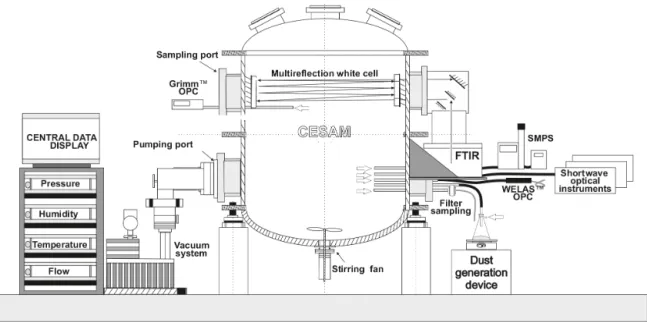
2 Experimental set-up and instrumentation
The schematic configuration of the CESAM set-up for the dust experiments is shown in Fig. 1. Prior to each experi-ment, the chamber was evacuated and kept at a pressure of 3×10⁻⁴hPa. Then, the reactor was filled with a mixture of 80 %N2 (produced by evaporation from a pressurized
liq-uid nitrogen tank, Messer, purity > 99.995 %) and 20 % O2
(Linde, 5.0). The chamber was equipped with a four-blade stainless steel fan to achieve homogeneous conditions within the chamber volume (with a typical mixing time of approx-imately 1 min). Mineral dust aerosols generated from parent soils were dispersed into the chamber and left in suspen-sion for a time period of 60–120 min, whilst monitoring of the evolution of their physico-chemical and optical proper-ties took place. The LW spectrum of the dust aerosols was measured by means of an in situ Fourier transform infrared (FTIR) spectrometer. Concurrently, the particle size distribu-tion and the SW scattering, absorpdistribu-tion, and extincdistribu-tion co-efficients were measured by several instruments sampling aerosols from the chamber. They include a scanning mobil-ity particle sizer (SMPS) and WELAS and SkyGrimm opti-cal particle counters for the size distribution, a nephelometer (TSI Inc. model 3563), an aethalometer (Magee Sci. model AE31), and two cavity-attenuated phase shift extinction an-alyzers (CAPS PMeX by Aerodyne) for aerosol SW optical properties. Dust samples were also collected on polycarbon-ate filters over the largest part of each experiment (47 mm Nuclepore, Whatman, nominal pore size 0.4 µm) for an anal-ysis of the particle mineralogical composition averaged over the length of the experiment.
Figure 1. Schematic configuration of the CESAM set up for the dust experiments. The dust generation (vibrating plate, Büchner flask containing the soil sample) and injection system is shown at the bottom on the right side. The position of the SMPS, WELAS, and SkyGrimm used for measuring the size distribution, FTIR spectrometer, SW optical instruments, and filter sampling system are also indicated.
and the related data properly corrected (Sect. 2.3.2). To com-pensate for the air being extracted from the chamber by the various instruments, a particle-freeN2–O2mixture was
con-tinuously injected into the chamber.
All experiments were conducted at ambient temperature and relative humidity < 2 %. The chamber was manually cleaned between the different experiments to avoid any car-ryover contaminations, as far as was possible. Background concentrations of aerosols in the chamber varied between 0.5 and 2.0 µg m−3.
In the following paragraphs we describe the system for dust generation, measurements of the dust LW spectrum, size distribution, and mineralogy, and data analysis. A sum-mary of the different measured and retrieved quantities in this study and their estimated uncertainties is reported in Table 1. Long-wave optical and size distribution data, acquired at dif-ferent temporal resolutions, are averaged over 10 min inter-vals. Uncertainties on the average values are obtained as the standard deviation over the 10 min intervals. A full descrip-tion of the SW optical measurements and results is out of the scope of the present study and will be provided in a forth-coming paper (Di Biagio et al., 2017).
2.1 Dust aerosol generation
In order to mimic the natural emission process, dust aerosols were generated by mechanical shaking of natural soil sam-ples, as described in DB14. The soils used in this study con-sist of the surface layer, which is subject to wind erosion in nature (Pye et al., 1987). Prior to each experiment, the soil samples were sieved to < 1000 µm and dried at 100◦C for about 1 h to remove any residual humidity. This
process-ing did not affect the mineral crystalline structure of the soil (Sertsu and Sánchez, 1978).
About 15 g of soil sample was placed in a Büchner flask and shaken for about 30 min at 100 Hz by means of a sieve shaker (Retsch AS200). The dust suspension in the flask was then injected into the chamber by flushing it with N2 at
10 L min−1for about 10–15 min, whilst continuously shak-ing the soil. Larger quantities of soil sample (60 g) mixed with pure quartz (60 g) had been used in DB14 to maximize the concentrations of the generated dust. The presence of the pure quartz grains increases the efficiency of the shaking, allowing a rapid generation of high dust concentrations. In that case it had been necessary, however, to pass the aerosol flow through a stainless steel settling cylinder to prevent large quartz grains from entering the chamber (DB14). For the present experiments, the generation system was optimized, i.e., the mechanical system used to fix the flask to the shaker was improved so that the soil shaking was more powerful, and sufficient quantities of dust aerosols could be generated by using a smaller amount of soil and without adding quartz to the soil sample. In this way, the settling cylinder could be eliminated. No differences were observed in the size distri-bution or mineralogy of the generated dust between the two approaches.
2.2 LW optical measurements: FTIR extinction spectrum
detector and a globar source. The FTIR spectrometer mea-sures between wavelengths of 2.0 (5000 cm−1) and 16 µm (625 cm−1)at 2 cm−1resolution (which corresponds to a res-olution varying from about 0.0008 at 2.0 µm wavelength to 0.05 µm at 16 µm) by co-adding 158 scans over 2 min. The FTIR spectrometer is interfaced with a multi-pass cell to achieve a total optical path length (x) within the chamber of 192±4 m. The FTIR reference spectrum was acquired immediately before the dust injection. In some cases small amounts of water vapor and CO2 entered CESAM during
particle injection and partly contaminated the dust spectra be-low 7 µm. This did not influence the state of particles as the chamber remained very dry (relative humidity < 2 %). Wa-ter vapor and CO2absorption lines were carefully subtracted
using reference spectra. The measured spectra were then in-terpolated at 0.02 µm wavelength resolution (which corre-sponds to a resolution varying from about 0.8 at 625 cm−1 wavenumber to 50 at 5000 cm−1). Due to the excessive loss of energy in the FTIR-measured transmission (T) from 2 to 3 and 15 to 16 µm, data were limited to the 3–15 µm interval. In this spectral range the dust spectral extinction coefficient
βextwas calculated as follows:
βext(λ)=
−ln(T (λ))
x . (1)
The uncertainty onβextwas calculated with the error
propa-gation formula by considering the uncertainties arising from
T noise (∼1 %) and from the standard deviation of the 10 min averages and of the path length x. We estimated it to be∼10 %.
In the 3–15 µm range, the dust extinction measured by the FTIR spectrometer is due to the sum of scattering and ab-sorption. Scattering dominates below 6 µm, while absorption is dominant above 6 µm. The FTIR multipass cell in the CE-SAM has been built following the White (1942) design (see Fig. 1). In this configuration, a significant fraction of the light scattered by the dust enters the FTIR detector and is not mea-sured as extinction. This is because mineral dust is dominated by the super-micron fraction, which scatters predominantly in the forward direction. As a consequence, the FTIR signal in the presence of mineral dust will represent only a fraction of dust scattering below 6 µm and almost exclusively absorp-tion above 6 µm. Figure S1 (Supplement), shows an example of the angular distribution of scattered light (phase function) and the scattering-to-absorption ratio calculated as a function of the wavelength in the LW for one of the samples used in this study. The results of the calculations confirm that above 6 µm the scattering signal measured by the FTIR spectrome-ter accounts for less than 20 % of the total LW extinction at the peak of the injection and less than 10 % after 120 min in the chamber. Consequently, we approximate Eq. (1) as fol-lows:
βabs(λ)≈
−ln(T (λ))
x (λ>6 µm). (2)
2.3 Size distribution measurements
The particle number size distribution in the chamber was measured with several instruments, based on different prin-ciples and operating in different size ranges:
– a scanning mobility particle sizer (SMPS; TSI, DMA Model 3080, CPC Model 3772; operated at 2.0/0.2 L min−1sheath–aerosol flow rates; 135 s resolu-tion), measuring the dust electrical mobility diameters (Dm, i.e., the diameter of a sphere with the same
mi-gration velocity in a constant electric field as the parti-cle of interest) in the range 0.019–0.882 µm. Given that dust particles have a density larger than unity (assum-ing an effective density of 2.5 g cm−3), the cut point of the impactor at the input of the SMPS shifts towards lower diameters. This reduces the range of measured mobility diameters to ∼ 0.019–0.50 µm. The SMPS was calibrated prior to the campaign with PSL particles (Thermo Sci.) of 0.05, 0.1, and 0.5 µm nominal diame-ters;
– a WELAS optical particle counter (Palas, model 2000; white light source between 0.35 and 0.70 µm; flow rate 2 L min−1; 60 s resolution), measuring the dust-sphere-equivalent optical diameters (Dopt, i.e., the diameter of a
sphere yielding on the same detector geometry the same optical response as the particle of interest) in the range 0.58–40.7 µm. The WELAS was calibrated prior to the campaign with Caldust 1100 (Palas) reference particles; – a SkyGrimm optical particle counter (Grimm Inc., model 1.129; 0.655 µm operating wavelength; flow rate 1.2 L min−1; 6 s resolution), measuring the dust-sphere-equivalent optical diameters (Dopt)in the range 0.25–
32 µm. The SkyGrimm was calibrated after the cam-paign against a “master” Grimm (model 1.109) just re-calibrated at the factory.
The SMPS and the WELAS were installed at the bottom of the chamber, while the SkyGrimm was installed at the top of the chamber on the same horizontal plane as the FTIR spectrometer and at about 60 cm across the chamber from the WELAS and the SMPS. As already discussed in DB14, measurements at the top and bottom of the chamber were in very good agreement during the whole duration of each experiment, which indicates a good homogeneity of the dust aerosols in the chamber.
2.3.1 Corrections of SMPS, WELAS, and SkyGrimm data
performed using the SMPS software. The electrical mobil-ity diameter measured by the SMPS was converted to a ge-ometrical diameter (Dg)by taking into account the particle
dynamic shape factor (χ ), as Dg=Dm/χ. The shape
fac-torχ, determined by comparison with the SkyGrimm in the overlapping particle range (∼0.25–0.50 µm), was found to be 1.75±0.10. This value is higher than those reported in the literature for mineral dust (1.1–1.6; e.g., Davies, 1979; Kaaden et al., 2008). The uncertainty in Dgwas estimated
with the error propagation formula and was∼6 %.
For the WELAS, optical diameters were converted to sphere-equivalent geometrical diameters (Dg)by taking into
account the visible complex refractive index. TheDopttoDg
diameter conversion was performed based on the range of values reported in the literature for dust in the visible range, i.e., 1.47–1.53 for the real part and 0.001–0.005 for the imag-inary part (Osborne et al., 2008; Otto et al., 2009; McConnell et al., 2010; Kim et al., 2011; Klaver et al., 2011). Optical calculations were computed over the spectral range of the WELAS using Mie theory for spherical particles by fixingn
at 1.47, 1.50, and 1.53, and by varyingkin steps of 0.001 be-tween 0.001 and 0.005. The spectrum of the WELAS lamp needed for optical calculations was measured in the labora-tory (Fig. S2). Dg was then set at the mean ±1 standard
deviation of the values obtained for the differentnandk. Af-ter calculations, the WELASDgrange became 0.65–73.0 µm
with an associated uncertainty of < 5 % forDg< 10 µm and
between 5 and 7 % at larger diameters. A very low counting efficiency was observed for the WELAS below 1 µm; thus data in this size range were discarded.
For the SkyGrimm, the Dopt to Dg diameter
conver-sion was performed with a procedure similar to that used for the WELAS. After calculations, the Dg range for the
SkyGrimm became 0.29–68.2 µm with an associated uncer-tainty < 15.2 % at all diameters. The inter-calibration be-tween the SkyGrimm and the master instrument showed rela-tively good agreement (< 20 % difference in particle number) atDg< 1 µm, but a large disagreement (up to 300 %
differ-ence) atDg> 1 µm. Based on inter-comparison data, a
recal-ibration curve was calculated for the SkyGrimm in the range
Dg< 1 µm, and the data for Dg> 1 µm were discarded. The
SkyGrimm particle concentration was also corrected for the flow rate of the instrument, which during the experiment was observed to vary between 0.7 and 1.2 L min−1 compared to its nominal value at 1.2 L min−1.
2.3.2 Correction for particle losses in sampling lines and determination of the full dust size
distribution at the input of each instrument In order to compare and combine extractive measurements (size distribution, filter sampling, and SW optics), particle losses due to aspiration and transmission in the sampling lines were calculated using the particle loss calculator (PLC) software (von der Weiden et al., 2009). Inputs to the software
include the geometry of the sampling line, the sampling flow rate, the particle shape factorχ, and the particle density (set at 2.5 g cm−3for dust).
Particle losses for the instruments measuring the number size distribution (SMPS, WELAS, and SkyGrimm) were cal-culated. This allowed the reconstruction of the dust size dis-tribution suspended in the CESAM that corresponds to the size distribution sensed by the FTIR spectrometer and that is needed for optical calculations in the LW. Particle loss was found to be negligible atDg< 1 µm, reaching 50 % at
Dg∼5 µm, 75 % atDg∼6.3 µm, and 95 % atDg∼8 µm for
the WELAS, the only instrument considered in the super-micron range. Data for the WELAS were then corrected as follows:
dN/d logDgCorr,WELAS=dN/d logDgWELAS/
×1−LWELAS Dg, (3)
where[dN/d logDg]WELASis the size measured by the
WE-LAS and LWELAS (Dg) is the calculated particle loss as
a function of the particle diameter. Data atDg> 8 µm, for
which the loss is higher than 95 %, were excluded from the dataset due to their large uncertainty. The uncertainty on
LWELAS(Dg)was estimated with a sensitivity study by
vary-ing the PLC software values of the input parameters within their uncertainties. TheLWELAS(Dg)uncertainty varies
be-tween ∼50 % at 2 µm and ∼10 % at 8 µm. The total un-certainty in the WELAS-corrected size distribution was esti-mated as the combination of the dN/d logDgstandard
devia-tion on the 10 min average and theLWELAS(Dg)uncertainty.
The full size distribution of dust aerosols within the CE-SAM, dN/d logDgCESAM, was determined by
combin-ing SMPS and SkyGrimm data with WELAS loss-corrected data: the SMPS was taken atDg< 0.3 µm, the SkyGrimm at
Dg=0.3–1.0 µm, and the WELAS atDg=1.0–8.0 µm. Data
were then interpolated in steps of dlogDg=0.05. An
exam-ple of the size distributions measured by the different instru-ments is shown in Fig. S3. Above 8 µm, where WELAS data were not available, the dust size distribution was extrapo-lated by applying a single-mode lognormal fit. The fit was set to reproduce the shape of the WELAS distribution between
Dg∼3–4 and 8 µm.
Particle losses in the filter sampling system (Lfilter (Dg))
were calculated estimating the size-dependent particles losses that would be experienced by an aerosol with the size distribution in CESAM reconstructed from the previous cal-culations. Losses for the sampling filter were negligible for
Dg< 1 µm, and increased to 50 % at Dg∼6.5 µm, 75 % at
Dg∼9 µm, and 95 % atDg∼12 µm. The loss function,Lfilter
(Dg), was used to estimate the dust size distribution at the
dN/d logDgfilter=dN/d logDgCESAM
×1−Lfilter Dg (4)
As a consequence of losses, the FTIR spectrometer and the filters sense particles over different size ranges. Figure S4 illustrates this point by showing a comparison between the calculated size distribution within CESAM and that sampled on filters for one typical case. An underestimation of the par-ticle number on the sampling filter compared to that mea-sured in CESAM is observed above 10 µm diameter. While the filter samples would underestimate the mass concentra-tion in the chamber, the relative proporconcentra-tions of the main min-erals should be well represented. As a matter of fact, at emis-sion, where particles of diameters above 10 µm are most rel-evant, the mineralogical composition in the 10–20 µm size class matches that of particles of diameters between 5 and 10 µm (Kandler et al., 2009). When averaging, and also tak-ing into account the contribution of the mass of the 10–20 µm size class to the total, differences in the relative proportions of minerals do not exceed 10 %.
2.4 Analysis of the mineralogical composition of the dust aerosol
The mineralogical composition of the aerosol particles col-lected on the filters was determined by combining the follow-ing techniques: X-ray diffraction (XRD, Panalytical model Empyrean diffractometer) to estimate the particles’ min-eralogical composition in terms of clays, quartz, calcite, dolomite, gypsum, and feldspars; wavelength dispersive x-ray fluorescence (WD-XRF, Panalytical PW-2404 spectrom-eter) to determine the dust elemental composition (Na, Mg, Al, Si, P, K, Ca, Ti, Fe;±8–10 % uncertainty); and X-ray ab-sorption near-edge structure (XANES) to retrieve the content of iron oxides (±15 % on the mass fraction) and their speci-ation between hematite and goethite. Half of the Nuclepore filters were analyzed by XRD and the other half by WD-XRF and XANES. Full details on the WD-XRF and XANES mea-surements and data analysis are provided elsewhere (Caponi et al., 2017). Here we describe the XRD measurements.
XRD analysis was performed using a Panalytical model Empyrean diffractometer with Ni-filtered CuKα radiation at 45 kV and 40 mA. Samples were scanned from 5 to 60◦ (2θ )in steps of 0.026◦, with a time per step of 200 s.
Sam-ples were prepared and analyzed according to the proto-cols of Caquineau et al. (1997) for low mass loadings (load deposited on filter < 800 µg). Particles were first extracted from the filter with ethanol, then concentrated by centrifug-ing (25 000 rpm for 30 min), diluted with deionized water (pH∼7.1), and finally deposited on a pure silicon slide.
For well crystallized minerals, such as quartz, calcite, dolomite, gypsum, and feldspars (orthoclase, albite), a mass calibration was performed in order to establish the relation-ship between the intensity of the diffraction peak and the
mass concentration in the aerosol samples, according to the procedure described in Klaver et al. (2011). The calibration coefficientsKi, representing the ratio between the total peak surface area in the diffraction spectra (Si)and the massmi of theith-mineral, are reported in Table S1 in the Supplement. The error in the obtained mass of each mineral was estimated with the error propagation formula taking into account the uncertainty inSi and the calibration coefficientsKi. The ob-tained uncertainty is±9 % for quartz,±14 % for orthoclase, ±8 % for albite,±11 % for calcite,±10 % for dolomite, and ±18 % for gypsum.
Conversely, the mass concentration of clays (kaolinite, il-lite, smectite, palygorskite, chlorite), also detected in the samples, cannot be quantified in absolute terms from the XRD spectra due to the absence of appropriate calibra-tion standards for these components (Formenti et al., 2014). Hence, the total clay mass was estimated as the difference between the total dust mass and the total mass of quartz, calcium-rich species, and feldspars, estimated after XRD calibration, and iron oxides, estimated from XANES. The mass of organic material was neglected in the calculation: its contributions, however, should not exceed 3 % according to the literature (Lepple and Brine, 1976). The total dust mass was calculated in two ways: from the particle size distribu-tiondN/d logDg
filter(Msize, by assuming a dust density of
2.5 g cm−3)and from the estimated elemental composition (Melemental, as described in Caponi et al., 2017). Our results
show thatMsizesystematically overestimatesMelemental. As a
result, usingMsizeorMelementalwould result in different clay
mass fractions. In the absence of a way to assess whether
MsizeorMelemental is more accurate, we decided to estimate
the clay mass for each dust sample as the mean±maximum variability of the values obtained by using the two mass es-timates,Msize andMelemental. This approach should give a
reasonable approximation of the average clay content in the dust samples. The error in the obtained clay mass varies in the range 14–100 %. Subsequently, the mass fraction for each mineral was estimated as the ratio of the mass of the mineral divided by the total mass of all minerals.
For the northern African and eastern Asian aerosols only, the mass apportionment between the different clay species was based on literature values of illite-to-kaolinite (I/K) and chlorite-to-kaolinite (Ch/I) mass ratios (Scheuvens et al., 2013; Formenti et al., 2014). For the other samples, only the total clay mass was estimated.
3 Retrieval of the LW complex refractive indices
coef-ficient, βabs(λ), measured in CESAM can be calculated as
follows:
(βabs(λ))calc= X
Dg
π D2g
4 Qabs m, λ, Dg
dN
d logDg
CESAM
d logDg, (5)
whereQabs (m,λ,Dg)is the particle absorption efficiency
andπ D
2 g 4
h dN d logDg
i
CESAMis the surface size distribution of the
particles. As the simplest approach, Qabs can be computed
using Mie theory for spherical particles.
Our retrieval algorithm consists of iteratively varying m
in Eq. (5) until (βabs(λ))calc matches the measured βabs(λ).
However, asmis a complex number with two variables, an additional condition is needed. According to electromagnetic theory,nandkmust satisfy the Kramers–Kronig (K–K) re-lationship (Bohren and Huffmann, 1983):
n (ω)−1= 2
πP
∞ Z
0
·k ()
2−ω2 ·d, (6)
withωthe angular frequency of radiation (ω=2π c/λ, (s−1)) and P the principal value of the Cauchy integral. Equa-tion (6) means that ifk(λ)is known, thenn(λ)can be calcu-lated accordingly. Hence, the K–K relation is the additional condition besides Eq. (5) to retrievenandk. A direct calcu-lation of the K–K integral is, however, very difficult as it re-quires the knowledge ofkover an infinite wavelength range. A useful formulation, which permits one to obtain the cou-ple ofn−kvalues that automatically satisfy the K–K condi-tion, is the one based on the Lorentz dispersion theory. In the Lorentz formulation,nandkmay be written as a function of the real (εr)and imaginary (εi)parts of the particle dielectric
function:
n (ω)=
1 2
q
(εr(ω))2+(εi(ω))2+εr(ω)
1/2
, (7a)
k (ω)=
1 2
q
(εr(ω))2+(εi(ω))2−εr(ω)
1/2
. (7b) In turn, εr(ω)andεi(ω)can be expressed as the sum ofN
Lorentzian harmonic oscillators:
εr(ω)=ε∞+ N X j=1 Fj
ω2j−ω2
ω2j−ω22+γ2 jω2
, (8a)
εi(ω)= N
X
j=1
Fjγjω
ωj2−ω22+γ2 jω2
, (8b)
whereε∞=n2visis the real dielectric function in the limit of
visible wavelengths,nvisthe real part of the refractive index
in the visible, andωj,γj, andFj are the three parameters (eigenfrequency, damping factor, and strength respectively) characterizing thejth oscillator.
In our algorithm we combined Eqs. (7a)–(7b) and (8a)– (8b) with Eq. (5) to retrieve n−k values that allow both the reproduction of the measured βabs(λ) and the
satisfac-tion of the K–K relasatisfac-tionship. In practice, in the iterasatisfac-tion procedure only one of the two components of the refrac-tive index (in our case, k) was varied, while the other (n) was recalculated at each step based on the values of the oscillator parameters (ωj,γj,Fj) obtained from a best fit for k. In the calculations, the initial value of k(λ) was set atk(λ)=λβabs(λ)/4π; then in the iteration procedure,k(λ)
was varied in steps of 0.001 without imposing any constraint on its spectral shape. Initial values of the (ωj,γj,Fj) pa-rameters were set manually based on the initial spectrum of
k(λ). Between 6 and 10 oscillators were needed to model the
k(λ)spectrum for the different cases. The fit betweenk(λ)
and Eq. (7b) was performed using the Levenberg–Marquardt technique. The iteration procedure was stopped when the condition: (|βabs(λ))calc−βabs(λ)|< 1 % was met at all
wave-lengths.
Optical calculations were performed between 6 and 15 µm, within a range where FTIR-measured scattering could be neglected (see Sect. 2.2). The uncertainties caused by this choice are discussed in Sect. 3.1. Below 6 µm,k(λ)was then fixed to the value obtained at 6 µm. Calculations were per-formed over 10 min intervals.
For each experiment and for each 10 min interval, the value ofnvisto use in Eq. (8a) was obtained from optical
cal-culations using the simultaneous measurements of the SW scattering and absorption coefficients performed in CESAM (Di Biagio et al., 2017). For the various aerosol samples con-sidered here, the value ofnvisvaried between 1.47 and 1.52
with an uncertainty < 2 %. This approach is better than the one used in DB14, where the value ofnviswas manually
ad-justed for successive trials. Specifically, in DB14,nvis was
varied and set to the value that allowed the best reproduction of the measured dust scattering signal below 6 µm. As dis-cussed in Sect. 2.2, however, only a fraction of the total dust scattering is measured by the FTIR spectrometer. As a result, the nvis values obtained in DB14 were considerably lower
than the values generally assumed for dust (nvis=1.32–1.35
compared to 1.47–1.53 from the literature; e.g., Osborne et al., 2008; McConnell et al., 2010), with a possible result-ing overall underestimation ofn. Here, instead, thenvisvalue
was obtained based on additional SW optical measurements, which ensured a more reliable estimate of the whole spectral
n.
al., 2009). The description and the results of the control ex-periment are reported in Appendix Sect. A.
3.1 Caveats on the retrieval procedure for the LW refractive index
The procedure for the retrieval of the complex refractive in-dex presented in the previous section combines optical calcu-lations, the Kramers–Kronig relation, and the Lorentz disper-sion theory, and was based on measurements of spectral ab-sorption and particle size distribution. The approach is quite sensitive to the accuracy and representativeness of the mea-surements and assumptions in the optical calculations. We now list the different points that need to be addressed to en-sure the accuracy of the retrieval procedure.
1. First, our optical calculations (Eq. 5) use Mie the-ory for spherical particles. This is expected to intro-duce some degrees of uncertainties in simulated LW spectra, especially near the resonant peaks (Legrand et al., 2014). However, as discussed in Kalashnikova and Sokolik (2004), deviations from spherical behavior are mostly due to the scattering component of extinction since irregularly shaped particles have larger scattering efficiencies than spheres. In contrast, particle absorp-tion is much less sensitive to particle shape. Given that our measured spectra are dominated by absorption, we can therefore reasonably assume that Mie theory is well suited to model our optical data. It also has to be pointed out that at present almost all climate models use Mie theory to calculate dust optical properties. So, with the aim of implementing our retrieved refractive indices in model schemes, it is required that the same optical as-sumptions are made in both cases, i.e., the optical the-ory used in models and that used for refractive index retrieval.
2. Second, as discussed in Sect. 2.2, measured dust spectra at wavelengths > 6 µm represent only dust absorption, with minimal contribution from scattering. Dufresne et al. (2002) show that the contribution of LW scattering from dust is quite important in the atmosphere, espe-cially under cloudy conditions. Therefore, the impact of neglecting the scattering contribution has to be assessed. The retrieval procedure used in this study is nearly in-dependent of whether dust extinction or absorption only is used. Indeed, the combination of Eq. (5) with the Lorentz formulation in Eq. (7a) and (7b) ensures the re-trieval ofn–kcouples that are theoretically correct (ful-filling the K–K relationship), and the specific quantity to reproduce by Eq. (5) – i.e., extinction or absorption – provides only a mathematical constraint on the retrieval. Therefore, neglecting the scattering contribution to the LW spectra has no influence on the estimates of the re-fractive index, and the real and the imaginary parts
ob-tained in this study represent both the scattering and the absorption components of the dust extinction.
3. Third, our optical calculations are performed only at wavelengths > 6 µm, while in the range 3–6 µmk(λ)is fixed to the value obtained at 6 µm. We examine the ac-curacy of this assumption. Given that, over the whole 3–6 µm range, dust is expected to have a negligible ab-sorption (kis close to zero; see Di Biagio et al., 2014a), fixingkat the value at 6 µm is a reasonable approxima-tion. Concerning the impact of this assumption on the retrieval ofn, it should be pointed out that in the range 3–6 µm, wherek is very low, the shape of then spec-trum is determined only by the anchor pointnvis, and
the exact value ofkis not relevant. 3.2 Uncertainty estimation
The uncertainty in the retrieved refractive index was esti-mated with a sensitivity analysis. Towards this goal,n and
kwere also obtained by using, as input to the retrieval algo-rithm, the measuredβabs(λ)and size distribution±their
esti-mated uncertainties. The differences between the so-obtained
nandkand the nandkfrom the first inversion were esti-mated. Then, we computed a quadratic combination of these different factors to deduce the uncertainty innandk.
The results of the sensitivity study indicated that the mea-surement uncertainties onβabs(λ)(±10 %) and the size
dis-tribution (absolute uncertainty on the number concentration, ±20–70 %, with values larger than 30 % found for diameters between about 0.5 and 2.0 µm) have an impact of∼10–20 % on the retrieval ofnandk.
Additionally, a sensitivity analysis was performed to test the dependence of the retrieved LW refractive index on the accuracy of the shape of the size distribution above 8 µm. As discussed in Sect. 2.3.2, the size distribution,
dN/d logDg
CESAM, used for the optical calculations was
measured between 0.1 and 8 µm based on SMPS, SkyGrimm, and WELAS data. However, it was extrapolated to larger sizes by applying a lognormal mode fit for particle diam-eters > 8 µm, where measurements were not available. The extrapolation was set to reproduce the shape of the WELAS size distribution betweenDg ∼3–4 and 8 µm. In the
sensitiv-ity study,nandkwere also obtained by using two different size distributions as input to the retrieval algorithm, in which the extrapolation curve atDg> 8 µm was calculated by
con-sidering the WELAS data±their estimatedy uncertainties. The results of the sensitivity study indicate that a change of the extrapolation curve between its minimum and maximum may induce a variation of less than 10 % on the retrievedn
andk.
The total uncertainty innandk, estimated as the quadratic combination of these factors, was close to 20 %.
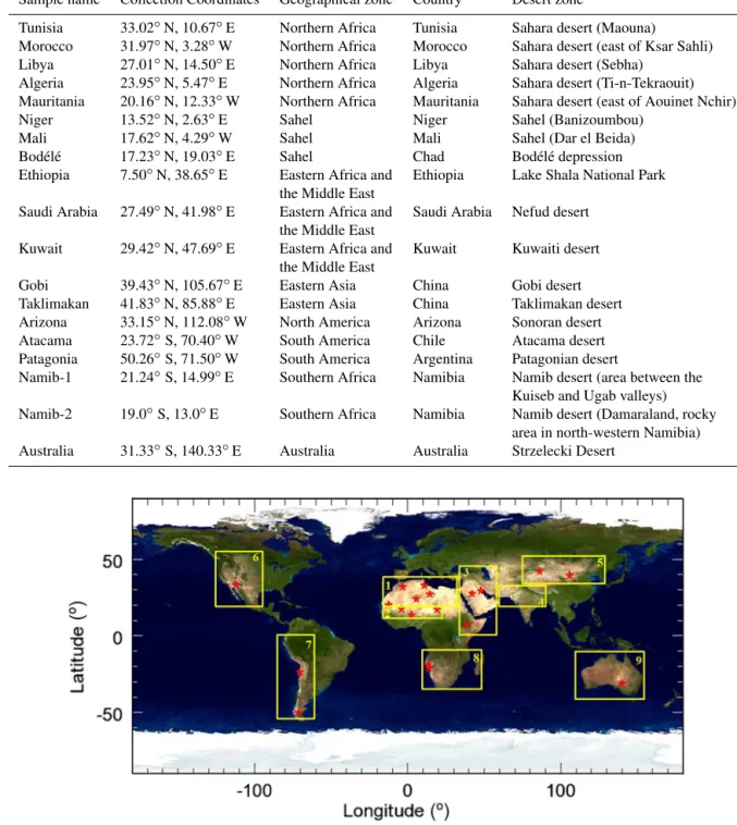
Table 2.Summary of information on the soil samples used in this study.
Sample name Collection Coordinates Geographical zone Country Desert zone
Tunisia 33.02◦N, 10.67◦E Northern Africa Tunisia Sahara desert (Maouna)
Morocco 31.97◦N, 3.28◦W Northern Africa Morocco Sahara desert (east of Ksar Sahli) Libya 27.01◦N, 14.50◦E Northern Africa Libya Sahara desert (Sebha)
Algeria 23.95◦N, 5.47◦E Northern Africa Algeria Sahara desert (Ti-n-Tekraouit) Mauritania 20.16◦N, 12.33◦W Northern Africa Mauritania Sahara desert (east of Aouinet Nchir) Niger 13.52◦N, 2.63◦E Sahel Niger Sahel (Banizoumbou)
Mali 17.62◦N, 4.29◦W Sahel Mali Sahel (Dar el Beida) Bodélé 17.23◦N, 19.03◦E Sahel Chad Bodélé depression Ethiopia 7.50◦N, 38.65◦E Eastern Africa and Ethiopia Lake Shala National Park
the Middle East
Saudi Arabia 27.49◦N, 41.98◦E Eastern Africa and Saudi Arabia Nefud desert the Middle East
Kuwait 29.42◦N, 47.69◦E Eastern Africa and Kuwait Kuwaiti desert the Middle East
Gobi 39.43◦N, 105.67◦E Eastern Asia China Gobi desert Taklimakan 41.83◦N, 85.88◦E Eastern Asia China Taklimakan desert Arizona 33.15◦N, 112.08◦W North America Arizona Sonoran desert Atacama 23.72◦S, 70.40◦W South America Chile Atacama desert Patagonia 50.26◦S, 71.50◦W South America Argentina Patagonian desert
Namib-1 21.24◦S, 14.99◦E Southern Africa Namibia Namib desert (area between the Kuiseb and Ugab valleys) Namib-2 19.0◦S, 13.0◦E Southern Africa Namibia Namib desert (Damaraland, rocky
area in north-western Namibia) Australia 31.33◦S, 140.33◦E Australia Australia Strzelecki Desert
Figure 2.Location (red stars) of the soil and sediment samples used to generate dust aerosols. The nine yellow rectangles depict the different global dust source areas as defined in Ginoux et al. (2012): (1) northern Africa, (2) the Sahel, (3) eastern Africa and Middle East, (4) central Asia, (5) eastern Asia, (6) North America, (7) South America, (8) southern Africa, and (9) Australia.
the choice of performing a single-mode extrapolation above 8 µm, which means neglecting the possible presence of larger dust modes.
4 Selection of soil samples: representation of the dust mineralogical variability at the global scale
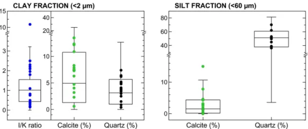
on the provenance of the selected soils is summarized in Ta-ble 2. Soils were grouped in the nine regions identified by Gi-noux et al. (2012): northern Africa, the Sahel, eastern Africa and Middle East, central Asia, eastern Asia, North America, South America, southern Africa, and Australia. The choice of which soils to analyze was made according to two criteria: (1) soils had to represent all major arid and semi-arid regions, as depicted by Ginoux et al. (2012) and (2) their mineralogy should envelop the largest possible variability of the soil min-eralogical composition at the global scale.
A large set of soils were available for northern Africa, the Sahel, eastern Africa and the Middle East, eastern Asia, and southern Africa. Here, the selection was performed using as guidance the global database of Journet et al. (2014), report-ing the composition of the clay (< 2 µm diameter) and silt (< 60 µm diameter) fractions in terms of 12 different als. Amongst them, we analyzed the variability of the miner-als that are most abundant in dust as well as most optically relevant to LW absorption, namely illite, kaolinite, calcite, and quartz in the clay fraction, and calcite and quartz in the silt fraction. The comparison of the clay and silt composi-tions of the soils extracted from the Journet database with the available samples resulted in the selection of five samples for northern Sahara, three for the Sahel, three for eastern Africa and the Middle East, and two for eastern Asia and southern Africa, as listed in Table 2. These soils constitute 15 of the 19 samples used in the experiments. More information on these soils is provided in the following.
For northern Africa, we selected soils from the north-ern Sahara (Tunisia, Morocco), which are richer in calcite and illite, central Sahara (Libya and Algeria), which are en-riched in kaolinite compared to illite and poor in calcite, and western Sahara (Mauritania), which are richer in kaolinite. The three samples from the Sahel are from Niger, Mali, and Chad (sediment from the Bodélé depression), and are en-riched in quartz compared to Saharan samples. The selected soils from northern Africa and the Sahel represent important sources for medium- and long-range dust transport towards the Mediterranean (Israelevich et al., 2002) and the Atlantic Ocean (Prospero et al., 2002; Reid et al., 2003). In particular, the Bodélé depression is one of the most active sources at the global scale (Goudie and Middleton, 2001; Washington et al., 2003).
The three soils from eastern Africa and the Middle East are from Ethiopia, Saudi Arabia, and Kuwait, which are im-portant sources of dust in the Red and Arabian seas (Prospero et al., 2002) and the North Indian Ocean (Leon and Legrand, 2003). These three samples differ in their content of calcite, quartz, and illite-to-kaolinite mass ratio (I/K).
For the second-largest global source of dust, eastern Asia, we considered two samples representative of the Gobi and the Taklimakan deserts, respectively. These soils differ in their content of calcite and quartz. Unfortunately, no soils are available for central Asia, mostly due to the difficulty of sampling these remote desert areas.
For southern Africa, we selected two soils from the Namib desert, one soil from the area between the Kuiseb and Ugab valleys (Namib-1) and one soil from the Damaraland rocky area (Namib-2), both sources of dust transported towards the south-eastern Atlantic (Vickery et al., 2013). These two soils present different compositions in term of calcite content and I/K ratio.
In contrast to Africa, the Middle East, and eastern Asia, a very limited number of samples were available in the soil collection for North and South America and Australia. Of the 19 soils used in our experiments, 4 were taken from these re-gions. These soils were collected in the Sonoran Desert for North America, in the Atacama and Patagonian deserts for South America, and in the Strzelecki desert for Australia. The Sonoran Desert is a permanent source of dust in North America, the Atacama desert is the most important source of dust in South America, whilst Patagonia emissions are rele-vant for long-range transport towards Antarctica (Ginoux et al., 2012). The Strzelecki desert is the seventh largest desert of Australia. No mineralogical criteria were applied to these areas.
A summary of the mineralogical composition of the 19 se-lected soils is shown in Fig. 3 in comparison with the full range of variability obtained considering the full data from the 9 different dust source areas. As illustrated by this fig-ure, the samples chosen for this study cover the entire global variability of the soil compositions derived by Journet et al. (2014).
5 Results
5.1 Atmospheric representativity: mineralogical composition
Figure 3.Box and whisker plots showing the variability of the soil composition in the clay and silt fractions at the global scale, i.e., by considering all data from the nine dust source areas identified in Fig. 2. Data are from the soil mineralogical database by Journet et al. (2014). Dots indicate specific mineralogical characteristics (illite-to-kaolinite mass ratio (I/K), calcite and quartz contents, extracted from Journet et al., 2014) of the soils used in the CESAM experiments, as listed in Table 2.
Figure 4.Mineralogy of the 19 generated aerosol samples considered in this study. The mass apportionment between the different clay species (illite, kaolinite, chlorite) is shown for northern African (Tunisia, Morocco, Libya, Mauritania, Niger, Mali, Bodélé) and eastern Asian (Gobi, Taklimakan) aerosols based on compiled literature values of the illite-to-kaolinite (I/K) and chlorite-to-kaolinite (Ch/I) mass ratios (Scheuvens et al., 2013; Formenti et al., 2014). For all other samples only the total clay mass is reported.
Morocco, and Gobi dusts. Conversely, only minor traces of dolomite (< 3 %) are detected in all the different samples. Finally, feldspars (orthoclase and albite) represent less than 15 % of the dust composition.
The observations from the present study capture well the global tendencies of the dust mineralogical compositions as observed in several studies based on aerosol field observa-tions, both from ground-based and airborne samples (e.g., Sokolik and Toon, 1999; Caquineau et al., 2002; Shen et al., 2005; Jeong, 2008; Kandler et al., 2009; Scheuvens et al., 2013; Formenti et al., 2014). For instance, at the scale of northern Africa, we correctly reproduce the geographi-cal distribution of geographi-calcite, which is expected to be larger in northern Saharan samples (Tunisia, Morocco), and very low or absent when moving towards the southern part of the
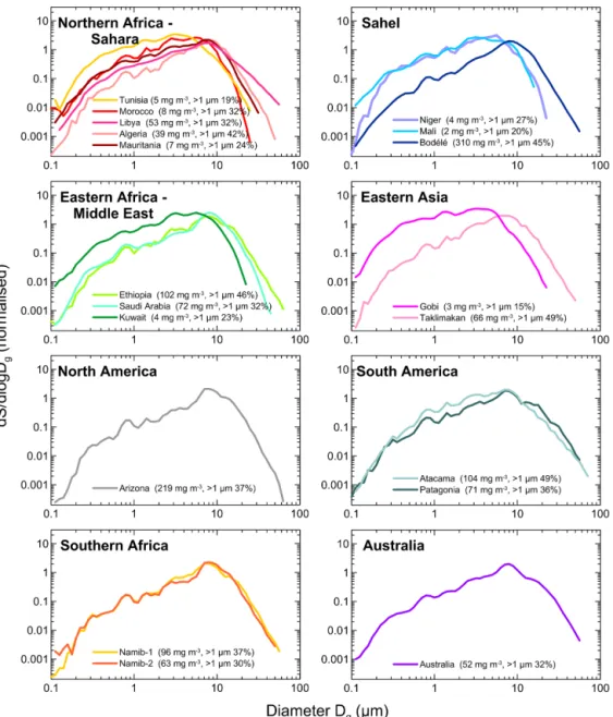
Ban-Figure 5.Surface size distributions in the CESAM at the peak of dust injection for all cases analyzed in this study; the total measured dust mass concentration and the percentage of the super-micron to sub-micron number fraction at the peak are also reported in the legend.
izoumbou during the AMMA (African Monsoon Multidis-ciplinary Analysis) campaign in 2006. The mineralogy for these samples was provided by Formenti et al. (2014). For a case of intense local erosion at Banizoumbou, they showed that the aerosol is composed of 51 % (by volume) clays, 41 % quartz, and 3 % feldspars. Our Niger sample, gener-ated from the soil collected at Banizoumbou, is composed of 51 % (±5.1 %; by mass) clays, 37 % (±3 %) quartz, and 6 % (±0.8 %) feldspars, in very good agreement with the field observations.
5.2 Atmospheric representativity: size distribution The size distribution of the dust aerosols measured at the peak of the dust injection in the chamber is shown in Fig. 5.
We report in the plot the normalized surface size distribution, defined as follows:
dS
d logDg
(normalized)= 1
Stot ·
π
4D
2 g
dN/d logDgCESAM
, (9)
with Stot the total surface area. The surface size
Figure 6. Comparison of CESAM measurements at the peak of the injection with dust size distributions from several airborne field campaigns in northern Africa. The grey shaded area represents the range of sizes measured in CESAM during experiments with the different northern African samples. Data from field campaigns are: AMMA (Formenti et al., 2011), SAMUM-1 (Weinzierl et al., 2009), and FENNEC (Ryder et al., 2013a). The shaded areas for each dataset correspond to the range of variability observed for the cam-paigns considered.
These values are comparable to what has been observed close to sources in proximity to dust storms (Goudie and Middle-ton, 2006; Rajot et al., 2008; Kandler et al., 2009; Marti-corena et al., 2010). Given that the protocol used for soil preparation and aerosol generation is always the same for the different experiments, the observed differences in both the shape of the size distribution and the mass concentration of the generated dust aerosols are attributable to the specific characteristics of the soils, which may be more or less prone to producing coarse-size particles.
The comparison of the chamber data with observations of the dust size distribution from several airborne campaigns in Africa is shown in Fig. 6. This comparison suggests that the shape of the size distribution in the chamber at the peak of the injection accurately mimics the dust distribution in the atmosphere near sources.
The time evolution of the normalized surface size distri-bution within CESAM is shown in Fig. 7 for two examples taken from the Algeria and Atacama experiments, while an example of the dust number and mass concentration evolu-tion over an entire experiment is illustrated in Fig. S5. The Algeria and Atacama samples were chosen as representative of different geographic areas and different concentration lev-els in the chamber. As shown in Fig. 7, the dust size distri-bution strongly changes with time due to gravitational set-tling: the coarse mode above 5 µm rapidly decreases, due to the larger fall speed at these sizes (∼1 cm s−1 at 10 µm, compared to ∼0.01 cm s−1 at 1 µm; Seinfeld and Pandis, 2006), and the relative importance of the fraction smaller than Dg=5 µm increases concurrently. In the chamber we
are thus able to reproduce very rapidly (in about 2 h) the size-selective gravitational settling, a process that in the
at-mosphere may take about 1 to 5 days to occur (Maring et al., 2003). In order to compare the dust gravitational set-tling in the chamber with that observed in the atmosphere, the following analysis was performed. For both Algeria and Atacama soils, the fraction of particles remaining in suspen-sion in the chamber as a function of time versus particle size was calculated as dNi(Dg)/dN0(Dg), where dNi(Dg)is the
number of particles measured by size class at timei(i cor-responding to 30, 60, 90, and 120 min after injection) and dN0(Dg) represents the size-dependent particle number at
the peak of the injection. The results of these calculations are shown in the lower panels of Fig. 7, where they are compared to the fraction remaining airborne after 1–2 days obtained in the field study by Ryder et al. (2013b) for mineral dust transported out of northern Africa in the Saharan air layer (Karyampudi et al., 1999), that is, at altitudes between 1.5 and 6 km above sea level. The comparison indicates that the remaining particle fraction observed 30 min after the peak of the injection is comparable to that obtained by Ryder et al. (2013b) for particles between∼0.4 and 3 µm for the Al-geria case, and∼0.4 and 8 µm for the Atacama case, but that the depletion is much faster for both smaller and larger par-ticles. This suggests, on the one hand, that the number frac-tion of coarse particles in the chamber depends on the ini-tial size distribution, that is, on the nature of the soil itself. On the other hand, it shows the limitation of the four-blade fan in providing a vertical updraft sufficient to counterbal-ance the gravimetric deposition for particles larger than about 8 µm. This point, however, is not surprising since it is clear that in the laboratory it is not possible to reproduce the wide range of dynamical processes that occur in the real atmo-sphere, and so to obtain a faithful reproduction of dust grav-itational settling and the counteracting re-suspension mech-anisms. Nonetheless, it should be noted that the rate of re-moval is higher at the earlier stages of the experiments than towards their end. The size-dependent particle lifetime, de-fined as the value at which dN/dN0is equal to 1/e(McMurry
and Rader, 1985), is relatively invariant for particles smaller thanDg<∼2 µm (> 60 min). This indicates that no
signif-icant distortion of the particle size distribution occurs after the most significant removal at the beginning of the exper-iment, and that the fine-to-coarse proportions are modified with time in a manner consistent with previous field observa-tions on medium- to long-transport (e.g., Maring et al., 2003; Rajot et al., 2008; Reid et al., 2008; Ryder et al., 2013b; Den-jean et al., 2016).
5.3 Dust LW extinction and complex refractive index spectra for the different source regions
wave-Figure 7.Upper panel: surface size distribution measured at the peak of the dust injection and at 30, 60, 90, and 120 min after injection for the Algeria and Atacama aerosols. The dust mass concentration is also indicated in the plot. Lower panel: fraction of particles remaining airborne in the chamber as a function of time versus particle size calculated as dNi(Dg)/dN0(Dg), where dNi(Dg)is the number of particles measured
by size class at timei(icorresponding to 30, 60, 90, and 120 min after injection) and dN0(Dg)represents the size-dependent particle number
at the peak of the injection. Values are compared to the estimate of Ryder et al. (2013b) for Saharan dust layers aged 1–2 days after emission.
length range, significant differences are observed when com-paring the samples, which in turn are linked to differences in their mineralogical composition.
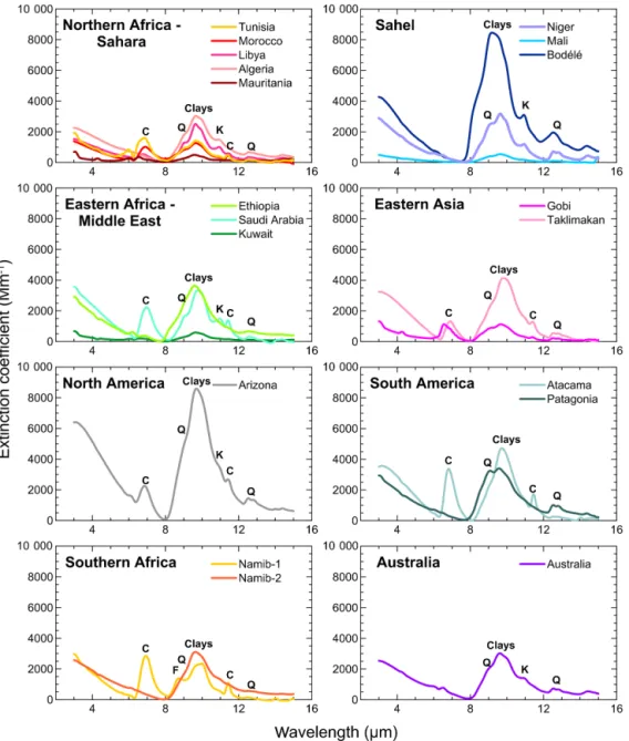
Figure 8 allows the identification of the spectral features of the minerals presenting the strongest absorption bands, in particular in the 8–12 µm atmospheric window (Table 3). The most prominent absorption peak is found around 9.6 µm for all samples, where clays have their Si–O stretch resonance peak. The shape around the peak differs according to the rel-ative proportions of illite and kaolinite in the samples, as is il-lustrated with the results for the Tunisia, Morocco, Ethiopia, Kuwait, Arizona, Patagonia, Gobi, and Taklimakan samples (richer in illite) compared to the Libya, Algeria, Mauritania, Niger, Bodélé, Saudi Arabia, and Australia samples (richer in kaolinite). Aerosols rich in kaolinite also show a secondary peak at ∼10.9 µm. The spectral signature of quartz at 9.2 and 12.5–12.9 µm is ubiquitous, with a stronger contribu-tion in the Bodélé, Niger, Patagonia, and Australia samples. Aerosols rich in calcite, such as the Tunisia, Morocco, Saudi Arabia, Taklimakan, Arizona, Atacama, and Namib-1 sam-ples show absorption bands at∼7 and 11.4 µm. Conversely, these are not present in the other samples and in particular in none of the samples from the Sahel. Finally, the contribution of feldspars (albite) at 8.7 µm is clearly detected only for the Namib-1 sample.
Table 3.Position of LW absorption band peaks (6–15 µm) for the main minerals composing dust. Montmorillonite is taken here as representative for the smectite family. For feldspars literature data are available only for albite.
Mineral species Wavelength (µm) Reference
Illite 9.6 Querry (1987)
Kaolinite 9.0, 9.6, 9.9, 10.9 Glotch et al. (2007) Montmorillonite 9.0, 9.6 Glotch et al. (2007) Chlorite 10.2 Dorschner et al. (1978) Quartz 9.2, 12.5–12.9 Peterson and Weinman (1969) Calcite 7.0, 11.4 Long et al. (1993)
Gypsum 8.8 Long et al. (1993)
Albite 8.7, 9.1, 9.6 Laskina et al. (2012)
Con-Figure 8.Dust extinction coefficient measured in the LW spectral range for the 19 aerosol samples analyzed in this study. Data for each soil refer to the peak of the dust injection in the chamber. Note that theyscale is different for northern Africa–the Sahara compared to the other cases. Main absorption bands by clays at 9.6 µm, quartz (Q) at 9.2 and 12.5–12.9 µm, kaolinite (K) at 10.9 µm, calcite (C) at 7.0 and 11.4 µm, and feldspars (F) at 8.7 µm are also indicated in the spectra.
versely, the lowest absorption is measured for the aerosols from Mauritania, Mali, Kuwait, and Gobi, for which the super-micron particle fraction and the mass concentrations are lower.
The intensity of the spectral extinction rapidly decreases after injection, following the decrease of the super-micron particle number and mass concentration. As an example, Fig. 9 shows the temporal evolution of the measured extinc-tion spectrum for the Algeria and Atacama aerosols. The in-tensity of the absorption band at 9.6 µm is about halved af-ter 30 min and reduced to ∼20–30 % and < 10 % of its ini-tial value after 60 and 90–120 min, respectively. Because of
Figure 9.Extinction spectra measured at the peak of the dust injection and at 30, 60, 90, and 120 min after injection for the Algeria and Atacama aerosols.
For both cases, the calculated ratios do not change signifi-cantly with time, i.e., they agree within error bars: for Al-geria, the quartz-to-clay ratio is 0.21±0.03 at the peak of the injection and 0.25±0.04 120 min later; for Atacama, the calcite-to-clay ratio is 0.73±0.10 and 0.67±0.09 for the same times. Similar results were also obtained for the other samples, with the exception of Saudi Arabia and Morocco, for which we observed an increase of the calcite-to-clay ra-tio with time. The time invariance of the quartz-to-clays and calcite-to-clays ratios observed for the majority of the an-alyzed aerosol samples agrees with the observations of the size-dependent dust mineralogical composition obtained by Kandler et al. (2009). These authors showed that in the super-micron diameter range up to∼25 µm, i.e., in the range where dust is mostly LW-active, the quartz-to-clay and calcite-to-clay ratios are approximately constant with size. This would suggest that the loss of particles in this size range should not modify the relative proportions of these minerals, and thus their contributions to LW absorption. Nonetheless, the differ-ent behavior observed for Saudi Arabia and Morocco would possibly indicate differences in the size-dependence of the mineralogical composition compared to the other samples.
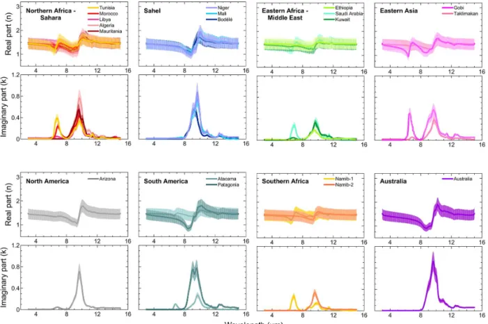
For each soil, the estimated real (n) and imaginary (k) parts of the complex refractive index are shown in Fig. 10. The reportednandkcorrespond to the mean of the 10 min val-ues estimated between the peak of the injection and 120 min later. This can be done because, for each soil, the time vari-ation of the complex refractive index is moderate. Standard deviations are < 10 % for n and < 20 % fork. The data in Fig. 10 are reported by considering as error the absolute un-certainty innandk, previously estimated at∼20 %. Figure 10 shows that the dust refractive index widely varies both in magnitude and spectral shape from sample to sample, fol-lowing the variability of the measured extinction spectra. The values for the real partnspan the range 0.84–1.94, while the imaginary partkis between∼0.001 and 0.92. The imaginary
part,k, is observed to vary both from region to region, and also within each region. The differences inkvalues obtained for different sources within the same region are in most cases larger than the estimatedkuncertainties. For specific regions (northern Africa, South America), the variability forkis of a similar order of magnitude to the variability at the global scale. Conversely, thenvalues mostly agree within error for all soils, both within a region and from one region to an-other. Exceptions are observed only at wavelengths where strong signatures from specific minerals are found in then
spectrum, as for example at 7 µm due to calcite (Saudi Ara-bia and Gobi samples), or that of quartz at 9.2 µm (Patagonia and Australia samples).
6 Discussion
6.1 Predicting the dust refractive index based on its mineralogical composition
Our results show that the LW refractive index of mineral dust, having different mineralogical compositions, varies consid-erably. Nevertheless, at wavelengths where the absorption peaks due to different minerals do not overlap, this variability can be predicted from the composition-resolved mass con-centrations. These considerations are illustrated in Fig. 11a, where we relate the mean values of the dustkin the calcite, quartz, and clay absorption bands between 7.0 and 11.4 µm to the percent mass fraction of these minerals in the dust. Mean
there-Figure 10.Real (n) and imaginary (k) parts of the dust complex refractive index obtained for the 19 aerosol samples analyzed in this study. Data correspond to the time average of the 10 min values obtained between the peak of the injection and 120 min later. The error bar corresponds to the absolute uncertainty innandk, estimated at∼ ±20 %.
fore measurable kvalues. Conversely, at 11.4 µm, non-zero
k values are obtained even in the absence of calcite, due to the interference of the calcite peak and the clay resonance bands. At this wavelength the correlation betweenkand the calcite mass fraction is also very low.
Poorer or no correlation is found betweenk and the per-cent mass fraction in the absorption bands of clays at 9.6 and 10.9 µm. This different behavior is not unexpected. Clay minerals such as kaolinite, illite, smectite, and chlorite are soil-weathering products containing aluminum and silicon in a 1:1 or 1:2 ratio (tetrahedral or octahedral structure, re-spectively). As a consequence, the position of their vibra-tional peaks is very similar (Dorschner et al., 1978; Querry, 1987; Glotch et al., 2007). In the atmosphere, these minerals undergo aging by gas and water vapor adsorption (Usher et al., 2003; Schuttlefield et al., 2007). As a result of the pro-duction conditions in the soils (weathering) and aging in the atmosphere, their physical and chemical conditions (com-position, crystallinity, aggregation state) might differ from one soil to another, and from that of mineralogical standards. That is the reason why XRD measurements of clays in nat-ural dust samples might be erroneous, and why we prefer to estimate the clay fraction indirectly. Nonetheless, the
in-direct estimate is also prone to error, and depends strongly on an independent estimate of the total mass (which, in the presence of large particles, can be problematic) as well as the correct quantification of the non-clay fraction. This is likely reflected in the large scatter observed in Fig. 11a when trying to relate thekvalue distribution to the corresponding percent mass of clays. These considerations also affect the specia-tion of clays, and explain the similar results obtained when separately plotting the spectralkvalues against the estimated kaolinite or illite masses. The superposition of the resonance bands of these two clays, as well as those of the smectites, which in addition are often poorly crystallized and therefore difficult to detect by XRD, as well as those in the quartz ab-sorption band at 9.2 µm, suggests that a more formal spectral deconvolution procedure based on single mineral reference spectra is needed to understand the shape and magnitude of the imaginary refractive index in this spectral band.
Figure 11.Imaginary part of the complex refractive index (k) versus the mineral content (in % mass) for the bands of calcite (7.0 and 11.4 µm), quartz (9.2 µm), and clays (9.6 and 10.9 µm). For the band at 9.6 µm the plot is drawn separately for total clays, and illite and kaolinite species. The linear fits are also reported for each plot. Linear fits were performed with the FITEXY.PRO Interactive Data Language (IDL) routine taking into account bothxandyuncertainties in the data. Same as Fig. 11a for the real part of the complex refractive index (n).
while for all other cases, very poor or no correlation is found. The real refractive index of dust is also almost constant at all bands (with the exception of that at 7.0 µm) regardless of the change in particle composition.
6.2 Dust complex refractive index versus size distribution during atmospheric transport
Quantifying the radiative impact of dust depends not only on the ability to provide spatially resolved optical properties, but also on the accurate representation of the possible changes of these properties during transport. In the LW, this effect is am-plified by the changes in the size distribution, particularly the loss of coarse particles. Our experiments accurately capture the overall features of the dust size distribution, including