N
o629
ISSN 0104-8910
Comparing Value–at–Risk Methodologies
Luiz Renato Lima, Breno de Andrade Pinheiro N ´eri
Os artigos publicados são de inteira responsabilidade de seus autores. As opiniões
neles emitidas não exprimem, necessariamente, o ponto de vista da Fundação
Comparing Value-at-Risk Methodologies
Luiz Renato Lima
∗Breno de Andrade Pinheiro N´
eri
†Graduate School of Economics - Get´
ulio Vargas Foundation
Rio de Janeiro, Brazil
October 26, 2006
Abstract
In this paper, we compare four different Value-at-Risk (V aR) method-ologies through Monte Carlo experiments. Our results indicate that the method based on quantile regression with ARCH effect dominates other methods that require distributional assumption. In particular, we show that the non-robust methodologies have higher probability to predict V aRs with too many violations. We illustrate our findings with an
em-pirical exercise in which we estimateV aRfor returns of S˜ao Paulo stock exchange index, IBOVESPA, during periods of market turmoil. Our re-sults indicate that the robust method based on quantile regression presents the least number of violations.
• JEL Classification: C52; C53, G15;
• Keywords: Time Series, Value-at-Risk, Quantile Regression.
∗E-mail: [email protected]
1
Introduction
Every day, financial institutions (like banks) estimate measures of market risk exposure, which are analyzed by the institutions’s decision makers. These esti-mates are also analyzed by internal and external auditors and regulatory agen-cies, who enforce that those institutions set aside enough capital to cover their risk exposures. This concern about market risk exposure has been increasing since the stock market crash in 1987, when 1 trillion of dollars (23% drop in value) was lost in a single day, known as the Black Monday. The recent tur-bulence in emerging markets, starting in Mexico in 1995, continuing in Asia in 1997, and spreading to Russia and Latin America in 1999, has further extended the interest in risk management.
Imprecise measures of risk cause inefficiencies: on one hand, if the measure is too conservative, then too much capital, that could be used in a more profitable way, is set aside; on the other hand, if it is too risky, then it yields a large number of violations, which may lead the institution to bankruptcy. Hence, researching for more and more reliable and accurate measure of risk methodologies is an active and growing literature.
Value-at-Risk (V aR) is probably the most used measure of risk since the 1996 amendment to the Basle Capital Accord which proposed that commercial banks with significant1trade activity could use their ownV aRmeasure to define
how much capital they should set aside to cover their market risk exposure, and U.S. bank regulatory agencies could audit theV aR methodology employed by the banks. This amendment was adopted in 1998 (Lopez, 1999)2. In Brazil, the
article 59 of the resolution N02.829, March 2001, of the Brazilian Central Bank
brings ”Para os seguimentos de renda fixa e de renda vari´avel dever´a ser feito o c´alculo do Valor em Risco (VaR) ...”, mandating the use of V aR to some markets.
Value-at-Risk is the loss in market value over a given time horizon that is exceeded with probabilityτ. That is, for a time series of returnsrt,findV aRt
such that
P[rt<−V aRt|It−1] =τ, (1)
whereIt−1 denotes the information set at timet−1. From this definition, it is
clear that finding aV aR essentially is the same as finding a 100τ% conditional quantile. Note that, for convention, the sign is changed to avoid negative num-ber in the V aRt(τ) time series. For regulatory purpose, τ is generally set to
1%. It does not mean that the banks may not estimateV aRs under different significance levels for their risk managers.
AlthoughV aRis a relatively simple concept, robust estimation of it is often ignored in practice. Indeed, one popular approach to estimate V aR assumes
1
Any bank or bank holding company whose trading activity equals greater than 10 percent of its total assets or whose trading activity equals greater than $1 billion must hold regulatory capital against their market risk exposure.
2
a conditionally normal return distribution. The estimation ofV aR is, in this case, equivalent to estimating conditional volatility of returns. Another popular method is to compute the empirical quantile nonparametrically, for example, rolling historical quantiles or Monte Carlo simulations based on an estimated model3.
However, these models are based on restricted assumptions about the distri-bution of returns. There has been accumulated evidence that portfolio returns (or log returns) are usually not normally distributed. In particular, it is fre-quently found that market returns display structural shifts, negative skewness and excess kurtosis in the distribution of the time series. This is particularly true in periods of market stress such as the financial crises faced by the Brazil-ian economy from 1997 to 2000. These market characteristics suggest that more robust methods are needed to estimateV aR.
In this paper, we estimate V aR using a robust method based on quantile regression model that allows for ARCH effect, and compare it to three other non-robustV aRmethodologies that are based on GARCH type volatility models. It is important to mention that Engle and Manganelli (1999) consider a different quantile regression based method. In particular, they consider an autoregression of the estimatedV aRs. Our approach, however, has the advantage of pursuing a well-developed distributional theory which facilitates statistical inference and computational optimization.
We are not the first ones to computeV aRusing a quantile regression model that allows for ARCH effect. In fact, Wu and Xiao (2002) used this model to estimate V aR and left-tail measures that were next employed to construct a risk-managed index fund. The performance of the ARCH Quantile method were then evaluated according to the capacity of the risk-managed index fund in tracking the S&P500 index.
There are, however, other ways to assess the quality of a V aR methodol-ogy. In this paper, we follow Engle and Manganelli (2001) who compareV aR
methodologies using descriptive statistics of the distributions of violations ob-tained via Monte Carlo simulations. Specifically, we simulate many trajectories of the return time series assuming different innovation distributions, and com-pute the number of violations4 using four different V aR methodologies. For
each simulated trajectory of the return series, we save the number of viola-tions. At the end of the experiment, we will have a distribution of the number of violations for each V aR methodology. Hence, we can compute descriptive statistics of the various distributions of violations and evaluate the quality of a
V aRmethodology according to these statistics.
Our Monte Carlo simulations indicate that the robust model based on quan-tile regression dominates other models that requires distributional assumptions. In particular, the distribution of violations generated from non-robust models are right-skewed and presents excess kurtosis, meaning that these non-robust models have high probability to present trajectories with too many violations.
3
This approach includes the weighted moving average method by J.P. Morgan’s Riskmetrics and the hybrid method by Boudoukh, Richardson, and Whitelaw (1998).
4
We illustrate our findings with an empirical application. We consider returns of the S˜ao Paulo stock exchange index, IBOVESPA, and show that the V aR
estimated by the quantile regression approach tends to predictV aRs more ac-curately during periods of market stress.
The outline of this paper is as follows: In Section 2, we describe the general framework and present the competing models. We describe our Monte Carlo experiment in Section 3. An empirical illustration is provided in Section 4, and Section 5 concludes.
2
The Competing Models
Most of the V aR methodologies are GARCH type models. Hence, they can be described using a GARCH framework (Giot and Laurent, 2004). GARCH models are designed to model the conditional heteroskedasticity in the time series of returnsyt, that is,
yt = µt+εt, (2)
εt = σtzt,
µt = c(η|It−1),
σt = h(η|It−1),
Wherec(η|It−1) and h(η|It−1) are functions of the vector of parametersη
and of the information setIt−1;ztis an independent and identically distributed
process, independent ofIt−1, withE[zt] = 0 andV ar[zt] = 1;µtis the
condi-tional mean foryt andσ2t is its conditional variance. The volatility model (2)
encompass a family of methodologies used to predictV aRs. We next describe some members of such family.
2.1
RiskMetrics
5RiskMetrics (J.P. Morgan, 1996) is the most simple analyzed methodology. However, it is still one of the most used model to compute V aR, and it is available for free by J.P. Morgan. In fact, RiskMetrics is a gaussian Integrated GARCH(1,1) model where the autoregressive parameter is set at a pre-specified value of 0.94 (for dailyV aR, in the United States) and the decay parameter (it can be viewed as an exponential filter in volatility) is set at 0.06, that is,
σt2= 0.06ε2t−1+ 0.94σ2t−1. (3)
The conditional meanµtis estimated by OLS, runningytagainst its own lags6,
andzt∼N(0,1). 5
RiskMetrics is a trademark by J.P. Morgan. 6
2.2
Gaussian GARCH(1,1)
In spite of using RiskMetrics, we could use the same GARCH(1,1) model but, instead of setting prespecified values of the parameters, we estimate them. In other words, we estimate the model
σ2t =ω+α1ε2t−1+β1σ2t−1, (4)
andzt∼N(0,1).
This is the second model to be analyzed in our Monte Carlo experiment. The Gaussian (or Normal) GARCH(1,1) is expected to generate better forecasts than RiskMetrics, because the parameters are estimated rather than prespecified.
Observe that these two first models do not capture neither the asymmetric dynamics7nor all the leptokurtosis that is generally present in macroeconomics
and financial time series, due to the fact that they assume normality for zt.
Indeed, in V aR applications, the choice of a appropriate distribution for the innovation processzt is an important issue as it directly affects the quality of
the estimation of the required quantiles. One way to weaken the assumption on the distribution ofzt is to consider the Skewed Student-t APARCH model,
which we describe next.
2.3
Skewed Student-t APARCH(1,1)
The APARCH (Ding, Granger and Engle, 1993) is an extension of the GARCH model that nests at least seven GARCH specifications. It can be described as
σtδ =ω+α1(|εt−1| −γ1εt−1)δ+β1σtδ−1, (5)
where ω, α1, γ1, β1 and δ (δ >0) are parameters to be estimated. δ plays
the role of a Box-Cox transformation ofσt, while γ1 (−1< γ1<1) reflects the
so-called leverage effect: the stylized fact that negative shocks impact volatility more than positive shocks.
Giot and Laurent (2003) and Giot (2003) use the above model considering a standardized version of the Skewed Student-t distribution - introduced by Fern´andez and Steel (1998) - for theztprocess. They show that such
standard-ized version provides more accurate V aR forecasts than the GARCH model. This result is somehow expected, because the Skewed Student-t APARCH(1,1) nests the Gaussian GARCH(1,1)8.
7
Beaudry and Koop (1993) showed that positive shocks to US GDP are more persistent than negative shocks, indicating asymmetric business cycle dynamics. More recently, Nam et al. (2005) identified asymmetric dynamics for daily return on the S&P 500 and used that to develop optimal technical trading strategies. In 1992, Brock, Lakonishok and LeBaron showed that two of the simplest and most popular trading rules - moving average and trading range break - consistently generate buy signals with higher returns than sell signals, and further, the returns following buy signals are less volatile than returns following sell signals.
8
According to Lambert and Laurent (2001) and provided that the degrees of freedomν >2, the innovation processztis said to follow a standardized Skewed
Student-t distributed, i.e. zt∼SKST(0,1, ξ, ν) if:
f(zt|ξ, ν) =
2 ξ+1
ξ
sg[ξ(szt+m)|ν] , ifzt<−ms 2
ξ+1
ξ
sghszt+m
ξ |ν i
, ifzt≥ −ms
, (6)
whereg[·|ν] is a symmetric (unit variance) Student-t density andξ >0 is the asymmetry coefficient. The parameters m and s2 are, respectively, the mean and the variance of the nonstandardized Skewed Student-t:
m=Γ
ν−1 2
√
ν−2
√
πΓ ν
2
ξ−1
ξ
(7)
and
s2=
ξ2+ 1
ξ2−1
−m2. (8)
In short, ξ models the asymmetry, while ν accounts for the tail thickness. See Lambert and Laurent (2001) for a discussion of the link between these two parameters and the skewness and the kurtosis.
2.4
ARCH(q) Quantile
Koenker and Zhao (1996) introduced the quantile regression model that allows for ARCH effect. The ARCH(q) Quantile methodology uses OLS estimator to estimate the conditional meanµt, but this is the only similarity with the first
three methodologies. The ARCH(q) Quantile does not assume any particular distribution to the processzt. The model can be described as follows
yt = µt+εt, (9)
εt = (γ0+γ1|εt−1|+...+γq|εt−q|)zt.
Thus, the ARCH(q) Quantile specification assumes that the errors follow an ARCH(q) type model9, in which the fundamental innovationz
t is drawn from
an unknown distributionFz.
In all the models presented in this paper, theV aR(τ) is defined as the τ th
conditional quantile of the return, that is
−V aRt(τ) =µt+Qε(τ|It−1), (10)
whereQε(τ|It−1) is the conditional quantile function ofεt.
Given a known distribution for the process zt, the computation of (10) is
straightforward. When the distribution ofztis unknown, we are led to the
prob-lem of quantile regression. The quantile regression method is an extension of the
9
empirical quantile methods. While classical linear regression methods, based on minimization of the sum of squared residuals, enable one to estimate models for conditional mean functions, quantile regression methods offer a mechanism for estimating models for the conditional quantile functions, like the one appearing in (10). Thus, quantile regression is capable of providing a complete statistical analysis of the stochastic relationships among random variables.
Moreover, quantile regression method has the important property that it is robust to distributional assumptions. This property is inherited from the robustness property of the ordinary sample quantiles. Quantile estimation is only influenced by the local behavior of the conditional distribution of the re-sponse variable near the specified quantile. As a result, the estimated condi-tional quantile function is not sensitive to outlier observations. Such a property is specially attractive in financial applications since many financial data such as IBOVESPA returns are usually heavy-tailed and thus are not (conditional) normally distributed
2.4.1 Quantile Regression
As we stated above, the idea of quantile regression provides a natural way of estimating Value-at-Risk. Quantile regression was introduced by Koenker and Basset (1978) and has received a lot of attention in econometrics research in the past two decades. To introduce quantile regression, letY be a random variable with distribution functionF(y). Theτ-th quantile ofY is defined by
QY (τ) = inf{y|F(y)≥τ}. (11)
Similarly, if we have a random sample{y1, y2, ..., yn} from the distributionF,
theτ-th sample quantile is:
ˆ
Qy(τ) = inf n
y|Fˆ(y)≥τo, (12)
where ˆF is the empirical distribution function of the random sample. This sample quantile may be found by solving the minimization problem:
min
b∈R
X
t∈{t:yt≥b}
τ|yt−b|+
X
t∈{t:yt<b}
(1−τ)|yt−b|
. (13)
Generalizing, if we consider the model:
yt=x′tb+ηt, (14)
wherext is akx1 vector of regressors including an intercept term. Then,
con-ditional on the regressorxt, theτ-th quantile of y:
QY (τ|xt) = inf{y|F(y|xt)≥τ}, (15)
is a linear function ofxt:
whereFε(·) is the cumulative distributional function of the residual. Theτ-th
conditional quantile ofy can be estimated by an analogue of equation (13):
ˆ
QY (τ|xt) =x′tˆb(τ), (17)
where
ˆb(τ) = arg min
b∈Rk
X
t∈{t:yt≥x′tb}
τ|yt−x′tb|+
X
t∈{t:yt<x′tb}
(1−τ)|yt−x′tb| (18)
is called the quantile regression. As a special case, the least absolute deviation (LAD) estimator (or l1 regression) is the median regression, i.e., the quantile
regression forτ= 0.5 10.
2.4.2 Estimating the ARCH Quantile V aR
Given equation (9), we denote (1,|εt−1|, ...,|εt−q|)′asXtand the corresponding
coefficient vector asγ. Then,
Qε(τ|It−1) =Xt′α(τ), (19)
where
α(τ) = (γ0Qz(τ), γ1Qz(τ), ..., γqQz(τ))′, (20)
andQz(τ) =Fz−1(τ) is the quantile function ofz. By definition,V aRt(τ), the
conditional Value-at-Risk at theτ-th quantile is just
−V aRt(τ) =µt+Xt′α(τ). (21)
So we need to estimateαb(τ)11. It can be achieved by solving the problem:
b
α(τ) = arg min
γ∈Rq+1
X
t∈{t:ut≥Z′tγ}
τ|εt−Xt′γ|+
X
t∈{t:ut<Zt′γ}
(1−τ)|εt−Xt′γ| .
(22) In practice, we can replaceεtby their OLS estimatorsbεt=yt−µbt. For example,
ifµt=βo+β1yt−1, thenbεt=yt−βbo−βb1yt−1, whereβbo andβb1are estimated
by OLS. Under mild regularity conditions, Koenker and Zhao (1996) show that
b
α(τ) estimated based onεbtis still a consistent estimator ofα(τ).
3
Monte Carlo Simulations
The objective of this section is to compare the four aforementionedV aR method-ologies. We perform Monte Carlo Simulations in which we generate 1000 time series with 1250 observations. We use a rolling window of 250 observations to
10
For more on quantile regression, see Koenker (2005). 11
estimate the parameters of the four methodologies and forecast theV aR(1%) associated to the 251st observation. The result is a 1-day-ahead V aR time
series, one for each methodology. At the end, we will have1001 forecast obser-vations for each methodology. We decide for a 250-observation window because it is the number of observations required to compute the multiplication factor
Ft in the Basle capital charge formula and because it is approximately 1 year,
a reasonable time to be used by the banks, containing enough information for the parameters estimation, without losing too many observations. To find the violations, we need to compare the last 1000 observations of the generated se-ries with the first 1000 observations of theV aR forecasts. The choice for the
V aR(1%) is due to regulatory purpose. The DGPs used in this experiment are
yt= 0.5yt−1+εt, (23)
εt=σtzt, (24)
σt2= 1 + 0.5ε2t−1+ψσ2t−1, (25)
wherezt are independent and identically distributed fundamental innovations,
zt∼i.i.d. There are five different innovation distributions, and we repeat the
experiment with GARCH effect (ψ= 0.5). Therefore, there are ten DGPs that are described below.
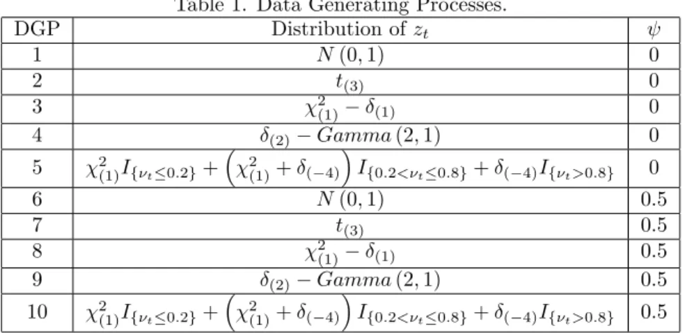
Table 1. Data Generating Processes.
DGP Distribution ofzt ψ
1 N(0,1) 0
2 t(3) 0
3 χ2
(1)−δ(1) 0
4 δ(2)−Gamma(2,1) 0
5 χ2(1)I{νt≤0.2}+
χ2(1)+δ(−4)
I{0.2<νt≤0.8}+δ(−4)I{νt>0.8} 0
6 N(0,1) 0.5
7 t(3) 0.5
8 χ2(1)−δ(1) 0.5
9 δ(2)−Gamma(2,1) 0.5
10 χ2(1)I{νt≤0.2}+
χ2(1)+δ(−4)
I{0.2<νt≤0.8}+δ(−4)I{νt>0.8} 0.5
where δ(x0) is the Dirac’s Delta density, which distributionFδ(x0)(x) which is
given by
Fδ(x0)(x) =
1,
0,
ifx≥x0
ifx < x0 , (26)
I{·}is an indicator function that values 1 if the condition inside the braces is true and 0 otherwise, andνtis an independent and identically distributed standard
uniform distribution,νt∼U[0,1].
finite expectation and variance), so zt presents leptokurtosis.The distribution
of zt in DGP3 is no longer symmetric. The distribution of zt in DGP4 and DGP5 are nonstandard (with mass points) and they are considered to verify
the robustness of V aR methodologies against distributional misspecification. GARCH effect is introduced inDGP6 toDGP10.
3.1
Results
For each replication (with 1000 daily forecasts), the ideal number of violations of aV aR(1%) is 10, but there are replications with more violations and there are replications with less violations. Hence, we shall analyze the distribution of the number of violations. Since there are 1000 replications, such a distribution of violations will have 1000 points (each point represents the number of violations that occurred in each trajectory). Recall that there are fourV aRmethodologies labelled as V aR i, i = 1,2,3,4. Hence, V aR 1, V aR 2, V aR 3, and V aR
4 correspond to the RiskMetrics, GARCH(1,1), APARCH(1,1), and ARCH(1) QuantileV aR methodologies, respectively. We assess the performance of each
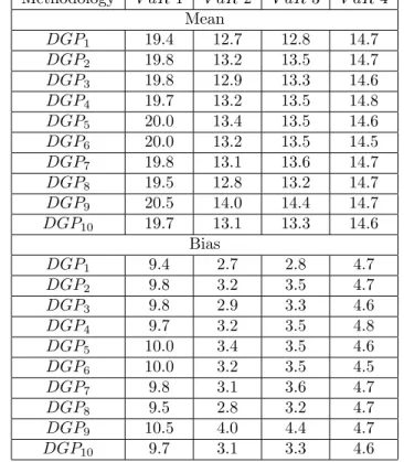
V aR methodology under the ten aforementioned DGPs. Tables 2, 3 and 4 present location and scale parameter estimates of the various distributions of violations.
Table 2. Distributions of violations: estimated mean and bias. Methodology V aR 1 V aR 2 V aR3 V aR4
Mean
DGP1 19.4 12.7 12.8 14.7
DGP2 19.8 13.2 13.5 14.7
DGP3 19.8 12.9 13.3 14.6
DGP4 19.7 13.2 13.5 14.8
DGP5 20.0 13.4 13.5 14.6
DGP6 20.0 13.2 13.5 14.5
DGP7 19.8 13.1 13.6 14.7
DGP8 19.5 12.8 13.2 14.7
DGP9 20.5 14.0 14.4 14.7
DGP10 19.7 13.1 13.3 14.6
Bias
DGP1 9.4 2.7 2.8 4.7
DGP2 9.8 3.2 3.5 4.7
DGP3 9.8 2.9 3.3 4.6
DGP4 9.7 3.2 3.5 4.8
DGP5 10.0 3.4 3.5 4.6
DGP6 10.0 3.2 3.5 4.5
DGP7 9.8 3.1 3.6 4.7
DGP8 9.5 2.8 3.2 4.7
DGP9 10.5 4.0 4.4 4.7
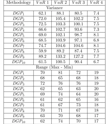
On one hand, we notice in Table 2 that all four methodologies present pos-itive estimated biases. The RiskMetrics methodology is the most biased and the Gaussian GARCH(1,1) has the least bias. The robust ARCH(1) Quantile method exhibits a very stable estimated bias across different innovation distri-butions. On the other hand, Table 3 shows that the variance is much higher (one order of magnitude higher) in the first three methodologies than in the ARCH(1) Quantile.
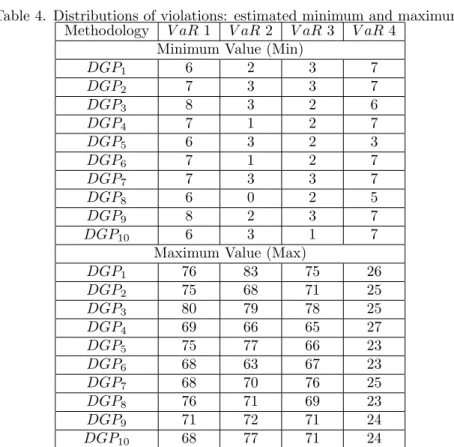
We compute in Table 3 the range of the distribution of the number of vi-olations, i.e., the difference between the maximum and the minimum number of violations. We notice that the fourth methodology has the lowest range. Indeed, as shown in Table 4, its maximum value never exceeds 27 violations, which can be considered a good performance in a V aR(1%). The non-robust methodologies have maximum number of violations at least three times as large as the ARCH(1) Quantile method. This excess dispersion invalidates the first threeV aRmethodologies, since they jeopardize the bank or institution that use them to computeV aR measures. It is not acceptable for a measure of risk to be too risky, in the sense that its probability of having trajectories with too many violations is too high. A bank may go belly-up if this trajectory is the true (realized) one.
Table 3. Distributions of violations: estimated variance and range. Methodology V aR 1 V aR 2 V aR3 V aR4
Variance
DGP1 62.1 88.1 80.5 7.4
DGP2 72.0 105.4 102.2 7.5
DGP3 72.5 103.3 100.1 7.5
DGP4 66.6 102.7 93.6 7.3
DGP5 69.0 102.1 98.7 8.1
DGP6 68.5 103.9 97.1 6.8
DGP7 74.7 104.6 104.6 8.1
DGP8 59.9 89.2 87.4 7.5
DGP9 89.2 133.2 127.2 7.7
DGP10 61.5 100.5 90.4 6.7
Range (Max - Min)
DGP1 70 81 72 19
DGP2 68 65 68 18
DGP3 72 76 76 19
DGP4 62 65 63 20
DGP5 69 74 64 20
DGP6 61 62 65 16
DGP7 61 67 73 18
DGP8 70 71 67 18
DGP9 63 70 68 17
On the other hand, the Gaussian GARCH(1,1) and the Skewed Student-t APARCH(1,1) present some trajectories with very few violations. In fact, the former has trajectories with no violations at all.
Table 4. Distributions of violations: estimated minimum and maximum. Methodology V aR 1 V aR 2 V aR3 V aR4
Minimum Value (Min)
DGP1 6 2 3 7
DGP2 7 3 3 7
DGP3 8 3 2 6
DGP4 7 1 2 7
DGP5 6 3 2 3
DGP6 7 1 2 7
DGP7 7 3 3 7
DGP8 6 0 2 5
DGP9 8 2 3 7
DGP10 6 3 1 7
Maximum Value (Max)
DGP1 76 83 75 26
DGP2 75 68 71 25
DGP3 80 79 78 25
DGP4 69 66 65 27
DGP5 75 77 66 23
DGP6 68 63 67 23
DGP7 68 70 76 25
DGP8 76 71 69 23
DGP9 71 72 71 24
DGP10 68 77 71 24
The ARCH(1) QuantileV aRexhibits the second greatest bias, but displays the lowest variance and range. To assess the trade-off between bias and variance, we adopt the Mean Squared Error (MSE), abiding by the formula (see Engle and Manganelli, 2001)
M SEXˆ:= 1
1000
1000X
i=1
(Xi−10)2, (27)
whereXiis the number of violation in thei-th replication, 1000 is the total
num-ber of replications and 10 is the ideal numnum-ber of violations, for aV aR(1%), at
each replication. It can be shown that theM SEXˆ=V arXˆ+BiasXˆ 2
,
whereBiasXˆ= ¯X−10 and ¯X = 10001 P1000i=1 Xi. The bias and the MSE are
show in Table 5.
Table 5. Distributions of violations: estimated Mean Squared Error. Methodology V aR 1 V aR 2 V aR3 V aR4
Mean Squared Error
DGP1 150.7 95.3 88.1 29.6
DGP2 168.8 115.4 114.6 29.5
DGP3 168.0 110.9 110.9 29.0
DGP4 160.9 112.7 106.1 30.3
DGP5 169.3 113.5 111.0 29.2
DGP6 167.9 113.7 109.0 27.0
DGP7 170.3 114.1 117.3 29.8
DGP8 151.0 97.1 97.6 29.2
DGP9 199.8 149.0 146.7 29.8
DGP10 155.0 109.8 101.3 28.0
We show in Table 6 estimates of skewness and excess kurtosis of the distri-butions of number of violations. We observe that the non-robustV aR method-ologies yield distributions of violations that are skewed to the right and possess excess kurtosis. Again, the robust ARCH(1) Quantile method gives rise to an well-behaved distribution of violations, with almost none skewness nor excess kurtosis.
Table 6. Distributions of violations: estimated skewness and excess kurtosis. Methodology V aR 1 V aR 2 V aR3 V aR4
Skewness
DGP1 2.8 3.2 3.3 0.3
DGP2 2.6 2.8 3.0 0.3
DGP3 2.7 3.0 3.1 0.3
DGP4 2.6 2.8 2.8 0.3
DGP5 2.6 2.8 2.7 0.1
DGP6 2.6 2.8 2.8 0.2
DGP7 2.7 2.9 2.9 0.2
DGP8 2.6 2.9 2.9 0.2
DGP9 2.4 2.6 2.6 0.2
DGP10 2.6 2.9 2.9 0.1
Excess Kurtosis
DGP1 10.1 11.6 11.9 0.2
DGP2 8.2 7.8 9.2 0.1
DGP3 8.5 8.9 10.4 0.2
DGP4 7.8 7.5 7.7 0.6
DGP5 8.3 7.8 7.2 0.1
DGP6 8.0 7.5 7.8 0.0
DGP7 8.5 8.2 8.8 0.1
DGP8 8.8 8.7 8.9 0.0
DGP9 6.1 6.2 6.4 0.0
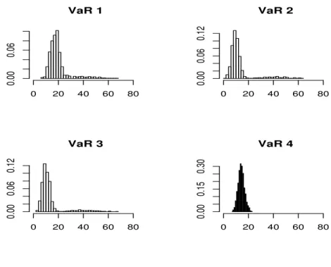
For completeness, we present the histograms of the number of violations for the four methodologies under the five DGPs with GARCH effect in Figures 1 to 5. It is clear that the non-robust methods present some trajectories with too many violations. Moreover, the estimated distribution of the number of violations is more concentrated in the fourth methodology, under all DGPs.
In sum, our Monte Carlo experiment suggests that the robust method dom-inates the other methods, since the former yields a distribution of number of violations that present very low MSE, almost none skewness and excess kurto-sis. More importantly, these nice properties are preserved over a wide range of innovation distributions, with or without GARCH effect. This result is expected because the robust method does not depend on distributional assumption.
Figure 1. Histograms of the number of violations under DGP 6.
VaR 1
0 20 40 60 80
0.00
0.06
VaR 2
0 20 40 60 80
0.00
0.06
0.12
VaR 3
0 20 40 60 80
0.00
0.06
0.12
VaR 4
0 20 40 60 80
0.00
0.15
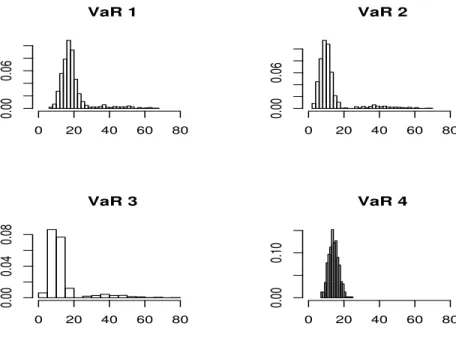
Figure 2. Histograms of the number of violations under DGP 7.
VaR 1
0 20 40 60 80
0.00
0.06
VaR 2
0 20 40 60 80
0.00
0.06
VaR 3
0 20 40 60 80
0.00
0.04
0.08
VaR 4
0 20 40 60 80
0.00
0.10
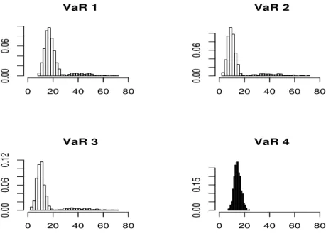
Figure 3. Histograms of the number of violations under DGP 8.
VaR 1
0 20 40 60 80
0.00
0.06
VaR 2
0 20 40 60 80
0.00
0.04
0.08
VaR 3
0 20 40 60 80
0.00
0.06
0.12
VaR 4
0 20 40 60 80
0.00
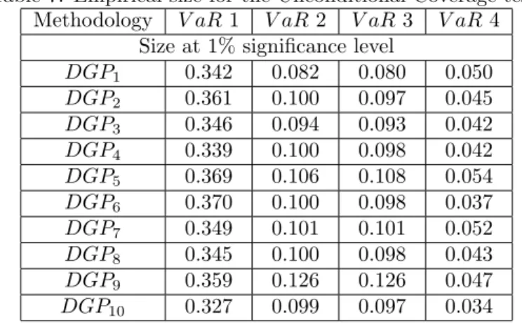
Figure 4. Histograms of the number of violations under DGP 9.
VaR 1
0 20 40 60 80
0.00
0.06
VaR 2
0 20 40 60 80
0.00
0.06
VaR 3
0 20 40 60 80
0.00
0.06
0.12
VaR 4
0 20 40 60 80
0.00
0.15
Figure 5. Histograms of the number of violations under DGP 10.
VaR 1
0 20 40 60 80
0.00
0.06
VaR 2
0 20 40 60 80
0.00
0.04
0.08
VaR 3
0 20 40 60 80
0.00
0.06
0.12
VaR 4
0 20 40 60 80
0.00
0.15
3.2
Backtest
The Unconditional Coverage backtest was proposed by Kupiec (1995). Under the null hypothesis thatP[rt<−V aRt(τ)|It−1] =τ,∀t, i.e., that the
proba-bility of occurrence of a violation is indeedτ, the number of violations, X, in a given time span, T, follows a binomial distribution: X ∼ Binomial(T, τ). Define ˆτ:= X
T. Then, the likelihood ratio test statistic 12is
LRuc= 2 ln
ˆ
τX(1−τˆ)T−X
τX(1−τ)T−X
!
. (28)
Under the null hypothesis thatτ= ˆτ,LRuc∼χ2(1).
Table 7 shows the probability of rejection, at 1% level of significance, of the null hypothesis of correct unconditional coverage,i.e., the hypothesis that the probability of the occurrence of a violation is indeed 1%. All the four method-ologies present an oversized test. However, the RiskMetric model is rejected in one third of the trajectories, approximately, while the ARCH Quantile VaR is rejected in 4% or 5% of the replications.
Table 7. Empirical size for the Unconditional Coverage test. Methodology V aR 1 V aR 2 V aR3 V aR4
Size at 1% significance level
DGP1 0.342 0.082 0.080 0.050
DGP2 0.361 0.100 0.097 0.045
DGP3 0.346 0.094 0.093 0.042
DGP4 0.339 0.100 0.098 0.042
DGP5 0.369 0.106 0.108 0.054
DGP6 0.370 0.100 0.098 0.037
DGP7 0.349 0.101 0.101 0.052
DGP8 0.345 0.100 0.098 0.043
DGP9 0.359 0.126 0.126 0.047
DGP10 0.327 0.099 0.097 0.034
4
An Empirical Illustration
4.1
The Data
We perform an empirical exercise using daily returns, in US dollars, of the Brazilian S˜ao Paulo Stock Exchange Index (IBOVESPA) from 08/07/1996 to 24/03/2000, summing up 920 observations. We choose this sample because we want to check the performance of each V aR methodology during periods of market turmoil. Indeed, the above sample period covers the Korean Crisis in 1997, the Russian crisis in 1999, and the blast of the technology-stock market bubble in 2000. Figure 6 displays the behavior of the IBOVESPA return over the above sample period.
12
Figure 6. IBOVESPA return time series.
IBOVESPA
time
Daily Return
0
200
400
600
800
−0.15
−0.05
0.05
0.15
It is well known that GARCH volatility models tend to predict implausible high V aR during periods of market turmoil. This happens because GARCH models treat both large positive and large negative return shocks as indicators of high volatility, which only large negative return shocks indicate higher Value-at-Risk. In other words, volatility andV aRare not the same thing, and this is not taken into account by the non-robust GARCH volatility models13. In contrast,
the robust ARCH Quantile, while predicting higher volatility in the ARCH component, assigns a much larger weight to a big negative return shock than to a big positive return shock and, thus, we expect that the resulting estimated
V aRs are closer to reality during periods of market turmoil (see similar argument in Wu and Xiao, 2002).
13
We next examine the distribution of the Ibovespa return. It was argued in this paper that, unlike the non-robust methods, the ARCH Quantile method has no need to specify the distribution of the innovation process,zt. The
impor-tance of this robustness aspect is revealed by the Quantile-Quantile plots (QQ plot). Recall that the QQ plot graphs the quantiles of the observed variable (IBOVESPA return) against the quantiles of a specified distribution. Hence, if the returns are distributed according to that specified distribution, then the points in the QQ-plots should lie alongside a straight line. The next two Fig-ures show the QQ plots against all the five innovation distributions used in our Monte Carlo experiment.
Figure 7. Q-Q Plot of the IBOVESPA return versus the Normal distribution.
● ●
● ●●●●●●●
●●●●●●● ●●●●●●
●
●●●●●●●●●●●●●●●●●●●●●●●●●●●●●●●●●●●●●●●●●●●●●●●●●●●●●●●●●●●●●●●●●●●●●●●●●●●●●●●●●●●●●●●●●●●●●●●●●●●●●●●●●●●●●●●●●●●●●●●●●●●●●●●●●●●●●●●●●●●●●●●●●●●●●●●●●●●●●●●●●●●●●●●●●●●●●●●●●●●●●●●●●●●●●●●●●●●●●●●●●●●●●●●●●●●●●●●●●●●●●●●●●●●●●●●●●●●●●●●●●●●●●●●●●●●●●●●●●●●●●●●●●●●●●●●●●●●●●●●●●●●●●●●●●●●●●●●●●●●●●●●●●●●●●●●●●●●●●●●●●●●●●●●●●●●●●●●●●●●●●●●●●●●●●●●●●●●●●●●●●●●●●●●●●●●●●●●●●●●●●●●●●●●●●●●●●●●●●●●●●●●●●●●●●●●●●●●●●●●●●●●●●●●●●●●●●●●●●●●●●●●●●●●●●●●●●●●●●●●●●●●●●●●●●●●●●●●●●●●●●●●●●●●●●●●●●●●●●●●●●●●●●●●●●●●●●●●●●●●●●●●●●●●●●●●●●●●●●●●●●●●●●●●●●●●●●●●●●●●●●●●●●●●●●●●●●●●●●●●●●●●●●●●●●●●●●●●●●●●●●●●●●●●●●●●●●●●●●●●●●●●●●●●●●●●●●●●●●●●●●●●●●●●●●●●●●●●●●●●●●●●●●●●●●●●●●●●●●●●●●●●●●●●●●●●●●●●●●●●●●●●●●●●●●●●●●●●●●●●●●●●●●●●●●●●●●●●●●●●●●●●●●●●●●●●●●●●●●●●●●●●●●●●●●●●●●●●●●●●●●●●●●●●●●●●●●●●●●●●●●●●●●●●●●●●●●●●●●●●●●●●●●●●●●●●●●●●●●●●●●●●●●●●●●●●●●●●●●●●●●●●●●●●●●●●●●●●●●●●●●● ●●●●●●●●
●●● ●
● ●
−4
−2
0
2
4
−0.15
−0.05
0.05
0.15
Q−Q Plot: Standard Gaussian
Theoretical Quantiles
Sample Quantiles
a Gaussian distribution. Figure 8 exhibits the QQ plots against the 4 remaining distributions. It seems that the student-t distribution with 3 degrees of freedom approximates the data distribution reasonably well, but there still be extreme positive and negative observations that lie off the straight line suggesting that the student-t distribution with 3 degrees of freedom does not fit the tail of the data distribution pretty well, what is particularly bad for risk measures. Figures 8 also shows that the data distribution departures from the other 3 distributions considered in our Monte Carlo experiment, but they fit the data distribution even worse than the previous two distributions.
Thus, given this uncertainty about the specification of the innovation distri-bution, how could we go about computing Value-at-Risk correctly? A natural answer to it is to use a method robust against distribution misspecification, such as the method based on the ARCH Quantile model.
Figure 8. Q-Q Plots of the IBOVESPA return versus the other distributions.
● ●●
● ● ●●●●●●●●●●●●●●●●●●●●●●●●●●●●●●●●●●●●●●●●●●●●●●●●●●●●●●●●●●●●●●●●●●●●●●●●●●●●●●●●●●●●●●●●●●●●●●●●●●●●●●●●●●●●●●●●●●●●●●●●●●●●●●●●●●●●●●●●●●●●●●●●●●●●●●●●●●●●●●●●●●●●●●●●●●●●●●●●●●●●●●●●●●●●●●●●●●●●●●●●●●●●●●●●●●●●●●●●●●●●●●●●●●●●●●●●●●●●●●●●●●●●●●●●●●●●●●●●●●●●●●●●●●●●●●●●●●●●●●●●●●●●●●●●●●●●●●●●●●●●●●●●●●●●●●●●●●●●●●●●●●●●●●●●●●●●●●●●●●●●●●●●●●●●●●●●●●●●●●●●●●●●●●●●●●●●●●●●●●●●●●●●●●●●●●●●●●●●●●●●●●●●●●●●●●●●●●●●●●●●●●●●●●●●●●●●●●●●●●●●●●●●●●●●●●●●●●●●●●●●●●●●●●●●●●●●●●●●●●●●●●●●●●●●●●●●●●●●●●●●●●●●●●●●●●●●●●●●●●●●●●●●●●●●●●●●●●●●●●●●●●●●●●●●●●●●●●●●●●●●●●●●●●●●●●●●●●●●●●●●●●●●●●●●●●●●●●●●●●●●●●●●●●●●●●●●●●●●●●●●●●●●●●●●●●●●●●●●●●●●●●●●●●●●●●●●●●●●●●●●●●●●●●●●●●●●●●●●●●●●●●●●●●●●●●●●●●●●●●●●●●●●●●●●●●●●●●●●●●●●●●●●●●●●●●●●●●●●●●●●●●●●●●●●●●●●●●●●●●●●●●●●●●●●●●●●●●●●●●●●●●●●●●●●●●●●●●●●●●●●●●●●●●●●●●●●●●●●●●●●●●●●●●●●●●●●●●●●●●●●●●●●●●●●●●●●●●●●●●●●●●●●●●●●●●●●●●●●●●●●●●●●●●●●●●●●●●●●●●●●●●●●●●●●●●●●●
● ●
−300 −100 0 100 200
−0.15
0.05
Q−Q Plot: t((3))
Theoretical Quantiles
Sample Quantiles ●●
● ● ● ● ● ● ● ● ● ● ● ● ● ● ● ● ● ● ● ● ● ● ● ● ● ● ● ● ● ● ● ● ● ● ● ● ● ● ● ● ● ● ● ● ● ● ● ● ● ● ● ● ● ● ● ● ● ● ● ● ● ● ● ● ● ● ● ● ● ● ● ● ● ● ● ● ● ● ● ● ● ● ● ● ● ● ● ● ● ● ● ● ● ● ● ● ● ● ● ● ● ● ● ● ● ● ● ● ● ● ● ● ● ● ● ● ● ● ● ● ● ● ● ● ● ● ● ● ● ● ● ● ● ● ● ● ● ● ● ● ● ● ● ● ● ● ● ● ● ● ● ● ● ● ● ● ● ● ● ● ● ● ● ● ● ● ● ● ● ● ● ● ● ● ● ● ● ● ● ● ● ● ● ● ● ● ● ● ● ● ● ● ●●●●●●●●●●●●●●●●●●●●●●●●●●●●●●●●●●●●●●●●●●●●●●●●●●●●●●●●●●●●●●●●●●●●●●●●●●●●●●●●●●●●●●●●●●●●●●●●●●●●●●●●●●●●●●●●●●●●●●●●●●●●●●●●●●●●●●●●●●●●●●●●●●●●●●●●●●●●●●●●●●●●●●●●●●●●●●●●●●●●●●●●●●●●●●●●●●●●●●●●●●●●●●●●●●●●●●●●●●●●●●●●●●●●●●●●●●●●●●●●●●●●●●●●●●●●●●●●●●●●●●●●●●●●●●●●●●●●●●●●●●●●●●●●●●●●●●●●●●●●●●●●●●●●●●●●●●●●●●●●●●●●●●●●●●●●●●●●●●●●●●●●●●●●●●●●●●●●●●●●●●●●●●●●●●●●●●●●●●●●●●●●●●●●●●●●●●●●●●●●●●●●●●●●●●●●●●●●●●●●●●●●●●●●●●●●●●●●●●●●●●●●●●●●●●●●●●●●●●●●●●●●●●●●●●●●●●●●●●●●●●●●●●●●●●●●●●●●●●●●●●●●●●●●●●●●●●●●●●●●●●●●●●●●●●●●●●●●●●●●●●●●●●●●●●●●●●●●●●●●●●●●●●●●●●●●●●●●●●●●●●●●●●●●●●●●●●●●●●●●●●●●●●●●●●●●●●●●●●●●●●●●●●●●●●●●●●●●●●●●●●●●●●●●●●●●●●●●●●●●●●●●●●●●●●●●●●●●●●●●●●●●●●●●●●●●●●●●●●●●●●●●●●●●●●●●●●●●●●●●●●●● ● ●
0 5 10 15 20 25 30
−0.15
0.05
Q−Q Plot: χχ((1)) 2 −− δδ
((1))
Theoretical Quantiles
Sample Quantiles
● ●●
●●●●●●●●●●●●●●●●●●●●●●●●●●●●●●●●●●●●●●●●●●●●●●●●●●●●●●●●●●●●●●●●●●●●●●●●●●●●●●●●●●●●●●●●●●●●●●●●●●●●●●●●●●●●●●●●●●●●●●●●●●●●●●●●●●●●●●●●●●●●●●●●●●●●●●●●●●●●●●●●●●●●●●●●●●●●●●●●●●●●●●●●●●●●●●●●●●●●●●●●●●●●●●●●●●●●●●●●●●●●●●●●●●●●●●●●●●●●●●●●●●●●●●●●●●●●●●●●●●●●●●●●●●●●●●●●●●●●●●●●●●●●●●●●●●●●●●●●●●●●●●●●●●●●●●●●●●●●●●●●●●●●●●●●●●●●●●●●●●●●●●●●●●●●●●●●●●●●●●●●●●●●●●●●●●●●●●●●●●●●●●●●●●●●●●●●●●●●●●●●●●●●●●●●●●●●●●●●●●●●●●●●●●●●●●●●●●●●●●●●●●●●●●●●●●●●●●●●●●●●●●●●●●●●●●●●●●●●●●●●●●●●●●●●●●●●●●●●●●●●●●●●●●●●●●●●●●●●●●●●●●●●●●●●●●●●●●●●●●●●●●●●●●●●●●●●●●●●●●●●●●●●●●●●●●●●●●●●●●●●●●●●●●●●●●●●●●●●●●●●●●●●●●●●●●●●●●●●●●●●●●●●●●●●●●●●●●●●●●●●●●●●●●●●●●●●●●●●●●●●●●●●●●●●●●●●●●●●●●●●●●●●●●●●●●●●●●●●●●●●●●●●●●●●●●●●●●●●●●●●●●●●●●●●●●●●●●●●●●●●●●●●●●●●●●●●●●●●●●●●●●●●●●●●●●●●●●●●●●●●●●●●●●●●●●●●●●●●●●●●●●●●●●●●●●●●●●●●●●●●●●●●●●●●●●●●●●●●●●●●●●●●●●●●●●●●●●●●●●●●●●●●●●●●●●●●●●●●●●●●●●●●●●●●●●●●●●●●●●●●●●●●●●●●●●●●●●● ●●
−20 −15 −10 −5 0
−0.15
0.05
Q−Q Plot: δδ((2))−Gamma(2,1)
Theoretical Quantiles
Sample Quantiles ●●
● ● ● ● ● ● ● ● ● ● ● ● ● ● ● ● ● ● ● ● ● ● ● ● ● ● ● ● ● ● ● ● ● ● ● ● ● ● ● ● ● ● ● ● ● ● ● ● ● ● ● ● ● ● ● ● ● ● ● ● ● ● ● ● ● ● ● ● ● ● ● ● ● ● ● ● ● ● ● ● ● ● ● ● ● ● ● ● ● ● ● ● ● ● ● ● ● ● ● ● ● ● ● ● ● ● ● ● ● ● ● ● ● ● ● ● ● ● ● ● ● ● ● ● ● ● ● ● ● ● ● ● ● ● ● ● ● ● ● ● ● ● ● ● ● ● ● ● ● ● ● ● ● ● ● ● ● ● ● ● ● ● ● ● ● ● ● ● ● ● ● ● ● ● ● ● ● ● ● ● ● ● ● ● ● ● ● ● ● ● ● ● ● ● ● ● ● ● ● ● ● ● ● ● ● ● ● ● ● ● ● ● ● ● ● ● ● ● ● ● ● ● ● ● ● ● ● ● ● ● ● ● ● ● ● ● ● ● ● ● ● ● ● ● ● ● ● ● ● ● ● ● ● ● ● ● ● ● ● ● ● ● ● ● ● ● ● ● ● ● ● ● ● ● ● ● ● ● ● ● ● ● ● ● ● ● ● ● ● ● ● ● ● ● ● ● ● ● ● ● ● ● ●●●●●●●●●●●●●●●●●●●●●●●●●●●●●●●●●●●●●●●●●●●●●●●●●●●●●●●●●●●●●●●●●●●●●●●●●●●●●●●●●●●●●●●●●●●●●●●●●●●●●●●●●●●●●●●●●●●●●●●●●●●●●●●●●●●●●●●●●●●●●●●●●●●●●●●●●●●●●●●●●●●●●●●●●●●●●●●●●●●●●●●●●●●●●●●●●●●●●●●●●●●●●●●●●●●●●●●●●●●●●●●●●●●●●●●●●●●●●●●●●●●●●●●●●●●●●●●●●●●●●●●●●●●●●●●●●●●●●●●●●●●●●●●●●●●●●●●●●●●●●●●●●●●●●●●●●●●●●●●●●●●●●●●●●●●●●●●●●●●●●●●●●●●●●●●●●●●●●●●●●●●●●●●●●●●●●●●●●●●●●●●●●●●●●●●●●●●●●●●●●●●●●●●●●●●●●●●●●●●●●●●●●●●●●●●●●●●●●●●●●●●●●●●●●●●●●●●●●●●●●●●●●●●●●●●●●●●●●●●●●●●●●●●●●●●●●●●●●●●●●●●●●●●●●●●●●●●●●●●●●●●●●●●●●●●●●●●●●●●●●●●●●●●●●●●●●●●●●●●●●●●●●●●●●●●●●●●●●●●●●●●●●●●●●●●●●●●●●●●●●●●●●●●●●●●●●● ● ●
−5 0 5 10 15 20 25 30
−0.15
0.05
Q−Q Plot: Contaminated Distribution
Theoretical Quantiles
Sample Quantiles
4.2
The Estimated VaRs
the results of our empirical illustration, it is important to mention that the comparison of differentV aR methodologies depends on the specification of µt
(the conditional mean) and the specifications of the conditional volatility. In the empirical example that follows, we considerµt=βo+β1yt−114. As for the
number of lags appearing in the definition ofεtin equation (9), we follow Wu
and Xiao (2002) and use a Wald test to determine the optimal lag choice15. As
for the order of the GARCH and APARCH models, we follow Enders (2003, pp 136) and use adjusted information criteria.
Table 8 shows the results of the Unconditional Coverage Test.
Table 8. Unconditional Coverage Test.
Methodology V aR 1 V aR2 V aR3 V aR 4 Number of Violations 14 12 13 11
Test StatisticLRuc 6.115232 3.429641 4.693915 2.335267
P-Value 0.013402 0.064036 0.030270 0.126473
Note that the number of violations in the RiskMetrics methodology is the greatest, while the ARCH(1) Quantile presents the greatest p-value in the Un-conditional Coverage test, that is to say, we do not reject, even at a 10% signif-icance level, the null hypothesis that the conditional probability of occurrence of a violation in this 1% Value-at-Risk estimated time series is indeed 1%. The GARCH(1,1) does not present a bad result, since we do not reject, at least at 5% significance level, the null hypothesis of correct unconditional coverage.
5
Conclusion
We perform a Monte Carlo experimet to compare four different Value-at-Risk
methodologies, RiskMetrics, Gaussian GARCH(1,1), Generalized Student-t APARCH(1,1), and ARCH(1) Quantile, under ten different data generating processes. The
ARCH(1) Quantile methodology does not assume any distribution for the re-turns, and this robustness is shown to avoid trajectories with too many viola-tions. The number of violations tends to be higher in the non-robust method-ologies.
We also perform an empirical exercise applying the four Value-at-Risk method-ologies to daily return of the IBOVESPA (measured in dollar values) in a period of market turmoil (1996-2000), when happens the Korean crisis, the Russian cri-sis and the blast of the technology-stock market bubble. We show again that the ARCH(1) Quantile methodology dominates the non-robust methodologies, in the sense that it presents the least number of violations.
14
First-order serial correlation in returns is not necessarily at odds with the efficient market hypothesis. See Campbell et al. (1997) for a detailed discussion.
15
A
Appendix: Computational Details
We use R and Ox to conduct this experiment. The former is an open source computer-programming language. Hence, it (and its source codes) can be freely downloaded from the Internet16. This availability keeps R always updated with the most recent techniques in Statistics, Econometrics and Computer Science. Ox can also be downloaded from internet for research purpose17.
The time series are generated in R because its default18 Random
Num-ber Generator (RNG) is the Mersenne-Twister (see Matsumoto and Nishimura, 1998), an impressive RNG with period 219937−1 and equidistribution in 623
consecutive dimensions (over the whole period).
This Monte Carlo experiment is extremely computational intensive. For each observation in theV aRforecast, there are three likelihood maximizations RiskMetrics, Gaussian GARCH(1,1) and Skewed Studentt APARCH(1,1) -with 250 observations (the window length) each. The third maximization oc-curs in a 7-dimensional hyperplane within a 8-dimensional space (5 parameters for the APARCH(1,1) specification and 2 parameters for the Skewed Student-t distribution). The R is supposed to take several months to conclude all the Monte Carlo, even in our server with 4 Intel Pentium IV Xeon at 2.8 GHz, a 4 GB RAM and a 100 GB SCSI Hard Disk running Linux Debian as Operating System. R is not so fast since it is an interpreted language: the interpreter executes the code line by line, so the user can enter a single line and see the results, which makes it more interactive and user-friendly. Ox is one order of magnitude faster than R since it is a compiled language: the compiler analyses the code as a whole, really optimizing it before executing it, which makes it much faster in large computations.
However, the ARCH(1) QuantileV aR must be estimated in R because the
quantreg package for R, version 3.82, May 15, 2005, developed mostly by Roger Koenker himself, is very complete and operational19. Thus, we proceed as
fol-lows: R generates the time series, then it calls Ox to estimate the first three
V aR methodologies20. Next, Ox returns these V aR forecasts to R, that
es-timates the ARCH(1) QuantileV aR, computes the descriptive statistics, and saves the results in the Hard Disk. R then generates another time series and the next replication begins. Using this hybrid solution (Ox and R), all the Monte Carlo experiment takes a couple of month. Every written code, for both R and Ox, used in this paper are available on www.fgv.br/alluno/bneri.
16
www.r-project.org 17
www.doornik.com 18
Alternatively, the user can select one of the eight RNGs available, or to supply another one.
19
Ox has also a code called rq to, at least, estimate quantile regression, but it is quite
incomplete. It was written by a Roger Koenker’s student, Daniel Morillo, but it has been abandoned in its version 1.0, August 1999.
20
References
[1] Basle Committee on Banking Supervision, 1996. Amendment to the Capital Accord to Incorporate Market Risks.
[2] Beaudry, P. and G. Koop, 1993. Do Recessions Permanently Change Out-put? Journal of Monetary Economics 31, 149-163.
[3] Box, G.E.P. and M.E. Muller, 1958. A Note on the Generation of Normal Random Deviates. Annals of Mathematical Statistics 29, 610-611.
[4] Boudoukh, J., M. Richardson, and R.F. Whitelaw, 1998. The Best of Both Worlds. Risk, 11, 64-67.
[5] Brazilian Central Bank, (March) 2001. Resolution N02.829.
[6] Brock, William, Josef Lakonishok and Blake LeBaron, December 1992. Simple Technical Trading Rules and the Stochastic Properties of Stock Returns. The Journal of Finance Vol. XLVII, N0 5.
[7] Campbell, John Y., Andrew W. Lo and A. Craig MacKinlay, 1997. The Econometrics of Finantial Markets. Princeton University Press.
[8] Chernozhukov, Victor and Umantsev, Len, 2001. Conditional Value-at-Risk: Aspects of Modelling and Estimation. Empirical Economics 26 (1), 271-292.
[9] Ding, Zhuanxin, Clive W. J. Granger and Robert F. Engle, 1993. A Long Memory Property of Stock Market Returns and a New Model. Journal of Empirical Finance 1, 83-106.
[10] Doornik, J.A., 2002. Object-Oriented Matrix Programming Using Ox. Tim-berlake Consultants Press and Oxford, 3rd ed., London.
[11] Enders, W., 2003. Aplied Econometric Time Series, 2nd edition. Wiley Series in Probability and Statistics.
[12] Engle, Robert F. and Simone Manganelli, 2001. Value-at-Risk Models in Finance. Working Paper 75, Working Paper Series, European Central Bank.
[13] Engle, Robert F. and Simone Manganelli, 1999. CAViaR: Conditional Au-toregressive Value at Risk by Regression Quantiles. University of California, San Diego, Working Paper.
[14] Engle, Robert F., 1982. Autoregressive Conditional Heteroskedasticity With Estimates of the Variance of U.K. Inflation. Econometrica 50, 987-1008.
[16] Giot, Pierre, 2003. The information content of implied volatility in agricul-tural commodity markets. Journal of Futures Markets 23, 441-454.
[17] Giot, Pierre and S´ebastien Laurent, 2003. Value-at-Risk for long and short positions. Journal of Applied Econometrics 18, 641-664.
[18] Giot, Pierre and S´ebastien Laurent, 2004. Modelling daily Value-at-Risk using realized volatility and ARCH type models. Journal of Empirical Fi-nance 11, 379-398.
[19] J. P. Morgan, December 17, 1996. RiskMetrics. J. P. Technical Document, Fourth Edition.
[20] Koenker, Roger, 2005. Quantile Regression. Econometric Society Mono-graphs.
[21] Koenker, Roger and G. Basset, 1978. Regression Quantiles. Econometrica 46, 33-50.
[22] Koenker, Roger and Q. Zhao,1996. Conditional Quantile Estimation and Inference for ARCH Models. Econometric Theory 12, 793-813.
[23] Kupiec, P., 1995. Techniques for Verifying the Accuracy of Risk Measure-ment Models. Journal of Derivatives 3, 73-84.
[24] Lambert, Philippe and S´ebastien Laurent, 2001. Modelling Financial Time Series Using GARCH-Type Models and a Skewed Student Density. Mimeo. Universit´e de Li`ege.
[25] Laurent, Sebastien and J.P. Peters, 2005. G@RCH 4.0, Estimating and Forecasting ARCH Models. Timberlake Consultants Press and Oxford, London.
[26] L’Ecuyer, Pierre, 1999. Tables of Maximally-Equidistributed Combined LFSR Generators. Mathematics of Computation 68, 261-269.
[27] Lopez, Jose A., 1999a. Regulatory Evaluation of Value-at-Risk Models. Journal of Risk 1, 37-64.
[28] Lopez, Jose A., 1999b. Methods for Evaluating Value-at-Risk Estimates. Federal Reserve Bank of San Francisco, Economic Review 2, 3-17.
[29] Marsaglia, George, 1997. A Random Number Generator for C. Discussion Paper, Posting on usenet newsgroup sci.stat.math.
[30] Marsaglia, George and A. Zaman, 1994. Some Portable Very-Long-Period Random Number Generators. Computers in Physics 8, 117-121.
[32] Nam, Kiseok, Kenneth M. Washer and Quantin C. Chu, 2005. Asymmetric Return Dynamics and Technical Trading Strategies. Journal of Banking & Finance 29, 391-418.
[33] Park S. and K. Muller, 1988. Random Number Generators: Good Ones Are Hard to Find. Communications of the ACM 31, 1192-1201.
´
Ultimos Ensaios Econˆomicos da EPGE
[604] Pedro Cavalcanti Gomes Ferreira e Leandro Gonc¸alves do Nascimento.Welfare and Growth Effects of Alternative Fiscal Rules for Infrastructure Investment in Brazil. Ensaios Econˆomicos da EPGE 604, EPGE–FGV, Nov 2005.
[605] Jo˜ao Victor Issler, Afonso Arinos de Mello Franco, e Osmani Teixeira de Carva-lho Guill´en. The Welfare Cost of Macroeconomic Uncertainty in the Post–War Period. Ensaios Econˆomicos da EPGE 605, EPGE–FGV, Dez 2005.
[606] Marcelo Cˆortes Neri, Luisa Carvalhaes, e Alessandra Pieroni. Inclus˜ao Digital e Redistribuic¸˜ao Privada. Ensaios Econˆomicos da EPGE 606, EPGE–FGV, Dez 2005.
[607] Marcelo Cˆortes Neri e Rodrigo Leandro de Moura. La institucionalidad del salario m´ınimo en Brasil. Ensaios Econˆomicos da EPGE 607, EPGE–FGV, Dez 2005.
[608] Marcelo Cˆortes Neri e Andr´e Luiz Medrado. Experimentando Microcr´edito: Uma An´alise do Impacto do CrediAMIGO sobre Acesso a Cr´edito. Ensaios Econˆomicos da EPGE 608, EPGE–FGV, Dez 2005.
[609] Samuel de Abreu Pessˆoa. Perspectivas de Crescimento no Longo Prazo para o Brasil: Quest˜oes em Aberto. Ensaios Econˆomicos da EPGE 609, EPGE–FGV, Jan 2006.
[610] Renato Galv˜ao Flˆores Junior e Masakazu Watanuki. Integration Options for Mercosul – An Investigation Using the AMIDA Model. Ensaios Econˆomicos da EPGE 610, EPGE–FGV, Jan 2006.
[611] Rubens Penha Cysne. Income Inequality in a Job–Search Model With Hetero-geneous Discount Factors (Revised Version, Forthcoming 2006, Revista Econo-mia). Ensaios Econˆomicos da EPGE 611, EPGE–FGV, Jan 2006.
[612] Rubens Penha Cysne. An Intra–Household Approach to the Welfare Costs of Inflation (Revised Version, Forthcoming 2006, Estudos Econˆomicos). Ensaios Econˆomicos da EPGE 612, EPGE–FGV, Jan 2006.
[613] Pedro Cavalcanti Gomes Ferreira e Carlos Hamilton Vasconcelos Ara´ujo. On the Economic and Fiscal Effects of Infrastructure Investment in Brazil. Ensaios Econˆomicos da EPGE 613, EPGE–FGV, Mar 2006.
[615] Aloisio Pessoa de Ara´ujo e Bruno Funchal. How much debtors’ punishment?. Ensaios Econˆomicos da EPGE 615, EPGE–FGV, Mai 2006.
[616] Paulo Klinger Monteiro. First–Price Auction Symmetric Equilibria with a Ge-neral Distribution. Ensaios Econˆomicos da EPGE 616, EPGE–FGV, Mai 2006.
[617] Renato Galv˜ao Flˆores Junior e Masakazu Watanuki.Is China a Northern Partner to Mercosul?. Ensaios Econˆomicos da EPGE 617, EPGE–FGV, Jun 2006.
[618] Renato Galv˜ao Flˆores Junior, Maria Paula Fontoura, e Rog´erio Guerra Santos.
Foreign direct investment spillovers in Portugal: additional lessons from a coun-try study. Ensaios Econˆomicos da EPGE 618, EPGE–FGV, Jun 2006.
[619] Ricardo de Oliveira Cavalcanti e Neil Wallace. New models of old(?) payment questions. Ensaios Econˆomicos da EPGE 619, EPGE–FGV, Set 2006.
[620] Pedro Cavalcanti Gomes Ferreira, Samuel de Abreu Pessˆoa, e Fernando A. Ve-loso. The Evolution of TFP in Latin America. Ensaios Econˆomicos da EPGE 620, EPGE–FGV, Set 2006.
[621] Paulo Klinger Monteiro e Frank H. Page Jr. Resultados uniformemente seguros e equil´ıbrio de Nash em jogos compactos. Ensaios Econˆomicos da EPGE 621, EPGE–FGV, Set 2006.
[622] Renato Galv˜ao Flˆores Junior. DOIS ENSAIOS SOBRE DIVERSIDADE CUL-TURAL E O COM ´ERCIO DE SERVIC¸ OS. Ensaios Econˆomicos da EPGE 622, EPGE–FGV, Set 2006.
[623] Paulo Klinger Monteiro, Frank H. Page Jr., e Benar Fux Svaiter.Exclus˜ao e mul-tidimensionalidade de tipos em leil˜oes ´otimos. Ensaios Econˆomicos da EPGE 623, EPGE–FGV, Set 2006.
[624] Jo˜ao Victor Issler, Afonso Arinos de Mello Franco, e Osmani Teixeira de Carva-lho Guill´en. The Welfare Cost of Macroeconomic Uncertainty in the Post–War Period. Ensaios Econˆomicos da EPGE 624, EPGE–FGV, Set 2006.
[625] Rodrigo Leandro de Moura e Marcelo Cˆortes Neri. Impactos da Nova Lei de Pisos Salariais Estaduais. Ensaios Econˆomicos da EPGE 625, EPGE–FGV, Out 2006.
[626] Renato Galv˜ao Flˆores Junior. The Diversity of Diversity: further methodolo-gical considerations on the use of the concept in cultural economics. Ensaios Econˆomicos da EPGE 626, EPGE–FGV, Out 2006.
[627] Maur´ıcio Canˆedo Pinheiro, Samuel Pessˆoa, e Luiz Guilherme Schymura. O Brasil Precisa de Pol´ıtica Industrial? De que Tipo?. Ensaios Econˆomicos da EPGE 627, EPGE–FGV, Out 2006.