❊♥s❛✐♦s ❊❝♦♥ô♠✐❝♦s
❊s❝♦❧❛ ❞❡
Pós✲●r❛❞✉❛çã♦
❡♠ ❊❝♦♥♦♠✐❛
❞❛ ❋✉♥❞❛çã♦
●❡t✉❧✐♦ ❱❛r❣❛s
◆◦ ✻✾✼ ■❙❙◆ ✵✶✵✹✲✽✾✶✵
❚❤❡ ❋♦r✇❛r❞✲ ❛♥❞ t❤❡ ❊q✉✐t②✲Pr❡♠✐✉♠ P✉③✲
③❧❡s✿ ❚✇♦ ❙②♠♣t♦♠s ♦❢ t❤❡ ❙❛♠❡ ■❧❧♥❡ss❄
❈❛r❧♦s ❊✉❣ê♥✐♦ ❞❛ ❈♦st❛✱ ❏♦ã♦ ❱✐❝t♦r ■ss❧❡r✱ P❛✉❧♦ ❋✳ ▼❛t♦s
❖s ❛rt✐❣♦s ♣✉❜❧✐❝❛❞♦s sã♦ ❞❡ ✐♥t❡✐r❛ r❡s♣♦♥s❛❜✐❧✐❞❛❞❡ ❞❡ s❡✉s ❛✉t♦r❡s✳ ❆s
♦♣✐♥✐õ❡s ♥❡❧❡s ❡♠✐t✐❞❛s ♥ã♦ ❡①♣r✐♠❡♠✱ ♥❡❝❡ss❛r✐❛♠❡♥t❡✱ ♦ ♣♦♥t♦ ❞❡ ✈✐st❛ ❞❛
❋✉♥❞❛çã♦ ●❡t✉❧✐♦ ❱❛r❣❛s✳
❊❙❈❖▲❆ ❉❊ PÓ❙✲●❘❆❉❯❆➬➹❖ ❊▼ ❊❈❖◆❖▼■❆ ❉✐r❡t♦r ●❡r❛❧✿ ❘❡♥❛t♦ ❋r❛❣❡❧❧✐ ❈❛r❞♦s♦
❉✐r❡t♦r ❞❡ ❊♥s✐♥♦✿ ▲✉✐s ❍❡♥r✐q✉❡ ❇❡rt♦❧✐♥♦ ❇r❛✐❞♦ ❉✐r❡t♦r ❞❡ P❡sq✉✐s❛✿ ❏♦ã♦ ❱✐❝t♦r ■ss❧❡r
❉✐r❡t♦r ❞❡ P✉❜❧✐❝❛çõ❡s ❈✐❡♥tí✜❝❛s✿ ❘✐❝❛r❞♦ ❞❡ ❖❧✐✈❡✐r❛ ❈❛✈❛❧❝❛♥t✐
❊✉❣ê♥✐♦ ❞❛ ❈♦st❛✱ ❈❛r❧♦s
❚❤❡ ❋♦r✇❛r❞✲ ❛♥❞ t❤❡ ❊q✉✐t②✲Pr❡♠✐✉♠ P✉③③❧❡s✿ ❚✇♦ ❙②♠♣t♦♠s ♦❢ t❤❡ ❙❛♠❡ ■❧❧♥❡ss❄✴ ❈❛r❧♦s ❊✉❣ê♥✐♦ ❞❛ ❈♦st❛✱
❏♦ã♦ ❱✐❝t♦r ■ss❧❡r✱ P❛✉❧♦ ❋✳ ▼❛t♦s ✕ ❘✐♦ ❞❡ ❏❛♥❡✐r♦ ✿ ❋●❱✱❊P●❊✱ ✷✵✶✵
✭❊♥s❛✐♦s ❊❝♦♥ô♠✐❝♦s❀ ✻✾✼✮
■♥❝❧✉✐ ❜✐❜❧✐♦❣r❛❢✐❛✳
The Forward- and the Equity-Premium
Puzzles: Two Symptoms of the Same Illness?
∗Carlos E. da Costa
Funda¸c˜ao Getulio Vargas
Jo˜ao V. Issler
Funda¸c˜ao Getulio Vargas
Paulo F. Matos
CAEN, Universidade Federal do Cear´a
July 15, 2009
Abstract
We build a pricing kernel using only US domestic assets data and check whether it accounts for foreign markets stylized facts that escape consumption based models. By interpreting our stochastic discount factor as the projection of a pricing kernel from a fully specified model in the space of returns, our results in-dicate that a model that accounts for the behavior of domestic assets goes a long way toward accounting for the behavior of foreign assets. We address predictabil-ity issues associated with the forward premium puzzle by: i)using instruments that are known to forecast excess returns in the moments restrictions associated with Euler equations, and; ii) by pricing Lustig and Verdelhan(2007)’s foreign currency portfolios. Our results indicate that the relevant state variables that ex-plain foreign-currency market asset prices are also the driving forces behind U.S. domestic assets behavior. Keywords: Equity Premium Puzzle, Forward Premium Puzzle, Return-Based Pricing Kernel. J.E.L. codes: G12; G15
1
Introduction
The Forward Premium Puzzle—henceforth, FPP—is how one calls the systematic departure from the intuitive proposition that, conditional on available information, the expected return to speculation in the forward foreign exchange market should be zero.
∗
First draft: July 2005. This paper has greatly benefited from comments and suggestions by
Caio Almeida, Marco Bonomo, Luis Braido, Ricardo Brito, Marcelo Fernandes, Jaime Filho, M´arcio
Garcia, Luiz Lima, Celina Ozawa, Rafael Santos, Andr´e Silva, seminar participants at EPGE, PUC-Rio, CAEN-UFC the XXVII SBE Meeting, “Econometrics in Rio”, the 2006 Meeting of the Brazilian
Finance Society, the 61th ESEM and the 1st Luso-Brazilian Finance Meeting. Matos acknowledges
One of the most acknowledged puzzles in international finance, the FPP was, in its infancy, investigated byMark(1985) within the framework of the consumption capital asset pricing model—CCAPM. Using a non-linear GMM approach, Mark estimated extremely high values for the representative agents’ risk aversion parameter, evidenc-ing the canonical consumption model’s inability to account for its over-identifyevidenc-ing restrictions. His results are similar to the ones found byHansen and Singleton(1982) and Hansen and Singleton (1984) with respect to the equity premium, an idea car-ried forward byMehra and Prescott (1985) who went on to propose what they have labelled the Equity Premium Puzzle—henceforth, EPP.
It may, at first, seem surprising that such similar results were never properly linked, and we may only conjecture why the literature on the FPP and the EPP drifted apart after the work of Mark.
First of all, proving that the two puzzles are related requires the existence of a consumption model which generates a pricing kernel that properly prices assets thus overcoming the shortcomings of previous models. Moreover, the existence of an early specificity for the FPP with no parallel in the case of the EPP—the predictability of returns based on interest rate differentials1—may have led many early researchers to believe that even if the CCAPM was capable of accounting for the equity premium it would not solve the FPP.
Indeed, representative of this latter point is the following quote fromEngel(1996) very comprehensive survey: “[...] it is tempting to draw parallels between the em-pirical failure of models of the foreign exchange premium, and the closed-economy asset pricing models. [...] However, the forward discount puzzle is not so simple as the equity premium puzzle. International economists face not only the problem that a high degree of risk aversion is needed to account for the estimated values of rpret
[rational expectations risk premium]. There is also the question of why the forward discount is such a good predictor ofst−1−ft[the difference between the (log of) next
period’s spot exchange rate and the (log of) forward rate associated with the same period]. There is no evidence that the proposed solutions to the puzzles in domestic financial assets can shed light on this problem.”
The purpose of this paper is to offer evidence to the contrary; that the solution
1We do not claim that returns on equity are not predictable. In fact, it is now established that
to the puzzle in domestic assets is likely to solve the problem in foreign-asset pricing. Our take on the FPP is that it is not only an international-economics issue, but an asset-pricing problem with important repercussions to monetary economics.2 Due to
the broad range of the two puzzles (FPP and EPP), and to the likely existence of a common explanation, we believe that the efficient approach for the profession is to join efforts in solving them. Our results invite researchers to refrain from diverting resources on the search of foreign-market specific shocks and concentrate on improving the performance of domestic asset-pricing models.
As of this moment, the question of what approach to adopt is still open. Recent work by Lustig and Verdelhan (2007), for example, tries to account for the forward premium behavior using a consumption based model. They build eight different for-eign assets portfolios using information on differential interest rates and compute pricing errors implied by a representative agent’s Euler Equation from a linear con-sumption model which they calibrate by borrowing structural parameters fromYogo (2006). Burnside(2007), however, disputes their empirical procedure, whileBurnside et al.(2007) argue, instead, that market microstructure issues underlie the behavior of international forward premia.
Our exercise cannot tell whether a consumption model does the job, nor does it allow one to tell whether microstructure issues are present in foreign exchange markets. It does, however, offer some support to the view that microstructure issues specific to foreign markets are not first order in generating the FPP, and that a single explanation (whether consumption based or not) should apply to domestic and foreign markets. We do this by getting as close as possible to finding an answer for the following question: had we written a model that successfully accounted for the behavior of domestic assets, would this model solve the forward premium puzzle?
Of course, a complete answer to this question cannot be given without actually writing down such model. What we do here is to devise a pricing-kernel estimate using only U.S. domestic assets, and show that such pricing kernel generates a risk premium able to accommodate the FPP. This suggests that the relevant state variables that drive foreign-currency market puzzles are already driving the behavior of U.S. domestic assets.
The return based kernel is the unique projection of a stochastic discount factor— henceforth, SDF—on the space of returns, i.e., the SDF mimicking portfolio. One
2
way to rationalize this SDF mimicking portfolio is to realize that it is the projection of a proper economic model (yet to be written) on the space of payoffs. Thus, the pricing properties of this projection are no worse than those of the proper model—a key insight ofHansen and Jagannathan(1991). An advantage of concentrating on the projection is that we can approximate it arbitrarily well in-sample using statistical methods and asset returns alone. Therefore, using such projection not only circum-vents the inexistence of a proper consumption model but is also guaranteed not to under-perform such ideal model.
In order to estimate the SDF mimicking portfolio on this paper, we employ the un-conditional linear multifactor model, which is perhaps the dominant model in discrete-time empirical work in finance.
Our main tests are based on Euler equations. We exploit the theoretical lack of correlation between discounted risk premia and variables in the conditioning set, or between discounted returns and their respective theoretical means, employing both discounted scaled excess-returns and discounted scaled returns in testing. We test the hypothesis that pricing errors are statistically zero and also scaled pricing errors using standard t-statistic, Wald, and over-identifying restriction tests in a generalized method-of-moments framework.
Our main results are clear cut: return-based pricing kernels built using U.S. assets alone, which account for domestic stylized facts, seem to account for the behavior of foreign assets as well. Hence, our SDF prices correctly the expected return to specu-lation in forward foreign-exchange markets for the widest group possible of developed countries with a long enough span of future exchange-rate data (Canada, Germany, Japan, Switzerland and the United Kingdom). It is important to stress the out-of-sample character of this exercise, avoiding a critique of in-out-of-sample over-fitting often used in this literature; see, e.g., Cochrane (2001). We also explicitly consider the eight dynamic foreign currency portfolios ofLustig and Verdelhan(2007).
defining features of the FPP. We also show that our U.S. based kernel is successful in pricing all but one ofLustig and Verdelhan(2007) portfolios.
These findings have also important implications for microstructure explanations for the behavior of the forward premium. First, because we have found a linear functional that prices foreign assets, our results rule out microstructure explanations that generate violations of the law of one price. Second, when we use only U.S. domestic assets in building our pricing kernel, and manage to explain the behavior of foreign assets we pose a serious challenge to any microstructure explanation that relies on specificities of foreign markets, e.g., Burnside et al.(2007).
The remainder of the paper is organized as follows. Section 2 gives an account of the literature that tries to explain the FPP and is related to our current effort. Section 3 discusses the techniques used to estimate the SDF and the pricing tests implemented in this paper. Section 4 presents the empirical results obtained in this paper. Concluding remarks are offered in Section 5.
2
Critical Appraisal of Current Debate on FPP
2.1 The puzzles and the CCAPM
Fama(1984) recalls that rational expectations alone does not restrict the behavior of forward rates, since it is always possible to include a risk-premium term that reconciles the time series behavior of the associated data. The relevant question is, thus, whether a theoretically sound economic model can offer a definition of risk capable of correctly pricing the forward premium.3
The natural candidate for a theoretically sound model for pricing risk is the CCAPM of Lucas (1978) and Breeden (1979). Assuming that the economy has an infinitely lived representative consumer, whose preferences are representable by a von Neumann-Morgenstern utility function u(·), the first order conditions for his(ers) optimal portfolio choice yields
1 =βEt
u′
(Ct+1)
u′(C
t)
Rit+1
∀i, (1)
3
and, consequently,
0 =Et
u′
(Ct+1)
u′
(Ct)
Rit+1−Rjt+1 ∀i, j, (2)
where β ∈(0,1) is the discount factor in the representative agent’s utility function,
Ri
t+1 andRjt+1 are, respectively, the real gross return on assets iand j at time t+ 1
and,Ct is aggregate consumption at time t. Under the CCAPM, βu′
(Ct+1)/u′(Ct), is a stochastic discount factor, i.e., a ran-dom variable that discount returns in such a way that their prices are simply the assets discounted expected payoffs. We shall use Mt+1 to denote SDF’s, be them
associated with the CCAPM or not.
Let the standing representative agent be a U.S. investor who can freely trade domestic and foreign assets.4 Next, define the covered,RC, and the uncovered return,
RU, on foreign government bonds trade as
RCt+1 = tFt+1(1 +i
∗
t+1)Pt
StPt+1
and RUt+1 = St+1(1 +i
∗
t+1)Pt
StPt+1
, (3)
where tFt+1 and St are the forward and spot prices of foreign currency in units of domestic currency, Pt is the dollar price level and i∗t+1, the nominal net return on a
foreign asset in terms of the foreign investor’s currency. Then, substitute RC forRi and RU forRj in (2) to get
0 =Et
u′
(Ct+1)
u′(C
t)
Pt(1 +i∗t+1)[tFt+1−St+1]
StPt+1
. (4)
Assuming u(C) = C1−α
(1−α)−1
, Mark (1985) applied Hansen (1982)’s Gener-alized Method of Moments (GMM) to (4). He estimated a coefficient of relative risk aversion, αb, above 40. He then tested the over-identifying restrictions to assess the validity of the model, rejecting them when the forward premium and its lags were used as instruments.5
4Here, we are implicitly assuming the absence of short-sale constraints or other frictions in the
economy. Our assumption is in contrast with that ofBurnside et al.(2007) for whom bid-ask spreads’ impact on the profitability of currency speculation plays the main role in generating the FPP.
5
Similar results were reported later by Modjtahedi (1991). Using a different, larger data set,
It is well known that similar results obtain when one considers the excess return of equity over risk-free short term bonds. In this case,Rti+1 = (1 +itSP+1)Pt/Pt+1 and
Rtj+1 = (1 +ib
t+1)Pt/Pt+1, in (2), where iSPt+1 is nominal return on S&P500 and ibt+1
nominal return on the U.S. Treasury Bill. This is the EPP in a nutshell.
Returns and Excess Returns When we substituteRC forRi and RU forRj,in
(1) we get
1 =Et
βu
′
(Ct+1)
u′(C
t)
tFt+1(1 +i∗t+1)Pt
StPt+1
and 1 =Et
βu
′
(Ct+1)
u′(C
t)
St+1(1 +i∗t+1)Pt
StPt+1
.
(5) In the canonical model, e.g., Hansen and Singleton (1982), Hansen and Singleton (1983) andHansen and Singleton(1984), the parameter of risk aversion is the inverse of the inter-temporal elasticity of substitution. Even if one is willing to accept high risk aversion, one must also be prepared to accept implausibly high and volatile interest rates.
Accordingly, if one wants to identify the structural parameterβ, in an econometric sense, one cannot resort to direct estimation of excess returns (e.g., 4), but rather to joint estimation of the two Euler equations for returns (e.g., 5), or to any linear rotation of them. It is, therefore, important to make a distinction between studies that test the over-identifying restrictions jointly implied by returns and those that test the ones implied by excess returns alone. For the latter no-rejection may be consistent withany value forβ, including inadmissible ones.6
In our view, a successful consumption-based model must account for asset prices everywhere (domestically and abroad), as well as price returns, excess returns, and many new facts recently found in the extensive empirical research that has been in a great deal sparked by the theoretical developments of the late seventies—see, for example, Cochrane(2006).
2.2 Our strategy and main issues
Even though important progress has been made in building more successful consump-tion models, there is no consensus as of this moment on whetherany model derived from the primitives of the economy accounts for either puzzle. The current state of the art, thus, precludes a direct answer to the question in the title of this paper.
6
Hence, we take an indirect approach.
We extract a pricing kernel from U.S. return data alone and show that it prices both the domestic and the foreign-exchange returns and excess returns.
Following Harrison and Kreps (1979), Hansen and Richard (1987), and Hansen and Jagannathan(1991), we write the system of asset-pricing equations,
1 =EtMt+1Rti+1
, ∀i= 1,2,· · ·, N. (6)
Given free portfolio formation, the law of one price guarantees, through Riesz repre-sentation theorem, the existence of a SDF,Mt+1 satisfying (6). Since (6) applies to
all assets,
0 =EthMt+1
Rit+1−Rjt+1i, ∀i, j. (7)
We combine statistical methods with the Asset Pricing Equation (6) to devise pricing-kernel estimates as projections of SDF’s on the space of returns, i.e., the SDF mimicking portfolio, which is unique even under incomplete markets. We denote the latter byM∗
t+1.
More specifically, our exercise consists in exploring a large cross-section of U.S. time-series stock returns to construct return-based pricing kernel estimates satisfying the Pricing Equation (6) for that group of assets. Then, we take these SDF estimates and use them to price assets not used in constructing them. Therefore, we perform a genuine out-of-sample forecasting exercise using SDF mimicking portfolio estimates, avoiding the in-sample over-fitting critique discussed inCochrane(2001), for example. We cannot overstress the importance of out-of-sample forecasting for our purposes. Our main point in this paper is to show that the forward- and the equity-premium puzzle are intertwined. Under the law of one price, a SDF that prices all assets exists, necessarily. Thus, an in-sample exercise would only provide evidence that the forward-premium puzzle is not simply a consequence of violations of the law of one price. We aim at showing more: a SDF can be constructed using only domestic assets, i.e., using the same source of information that guides research regarding the equity premium puzzle, and still price foreign assets. It is our view that this SDF is to capture the growth of the marginal utility of consumption in a model yet to be written.
fully specifying a model for the pricing kernel by treating the return on a benchmark portfolio as a latent variable.7 Also,Korajczyk and Viallet(1992) apply the arbitrage pricing theory—APT—to a large set of assets from many countries, and test whether including the factors as the prices of risk reduces the predictive power of the forward premium. They do not, however, perform out-of-sample exercises and do not try to relate the two puzzles.
Backus et al. (1995) ask whether a pricing kernel can be found that satisfies, at the same time, log-linearized versions of
0 =Et
M∗
t+1
Pt(1 +i∗t+1)[tFt+1−St+1]
StPt+1
(8)
and
Rft = 1 Et(M∗
t+1)
, (9)
where Rtf is the risk-free rate of return. The nature of the question we answer is similar, albeit enlarging its scope by considering all the main domestic assets and focusing on much richer instrument sets.8
Microstructure and the FPP Burnside et al. (2007) investigate the role played
by microstructure issues on generating the FPP. They argue that currency markets are thin and characterized by important transaction costs. They show that bid-ask spreads are not negligible and that price pressures are also important in understanding the persistence of apparently unexplored opportunities in those markets.
Large bid-ask spreads generate violations of the law of one price, which are incom-patible with the existence of a linear pricing functional. Price pressure, introduces a wedge between average and marginal Sharpe ratios. This allows for the presence of observed opportunities that cannot be accounted for by risk but that cannot be exploited without affecting prices. While our approach allows us to rule out violations of the law of one price,9 we cannot rule out microstructure explanations that do not
7Their results met with partial success: all these papers reject the unbiasedness hypothesis but are
in conflict with each other with regards to the rejection of restrictions imposed by the latent-variable model. However, contrary to what we do here, this line of research does not try to relate the EPP and the FPP.
8
Anticipating our results, we should emphasize that we do not reject (9) for any of the instruments, as well, which means that our SDF satisfies both conditions presented byBackus et al.(1995).
9
generate such violations. However, the fact that we construct our pricing kernel using domestic assets poses a challenge toBurnside et al. (2007)’s explanation.
To make our point as stark as possible, assume that there are two different markets, labelled market 1 and 2, respectively. Market 1 is assumed to be a frictionless thick markets, while market 2 is subject to price pressure. Without redundant assets, the law of one price cannot be violated, at least in the usual sense: we cannot use such argument to rule out the possibility of finding a pricing kernel that prices both assets. Assume the existence of a representative agent who invests in both assets and which investment problem we may write, in the case of a two period setting, as
max A1,A2
u(W −p1A1−p2(A2)A2) +βEu
A1˜δ1+A2δ˜2
,
where ˜δi,i= 1,2, are the payoffs of assets in markets 1 and 2. The price in market 1, is p1, while function p2(·) represents the way the agent perceives how prices on the
market with frictions are affected by his(er) positions. This function captures the fact that the agent realizes that he(she) cannot take large positions on assets in market 2 without affecting their prices. To simplify notation we assume that there is only one asset in this market.
Our procedure to extract a pricing kernel from domestic assets, which we as-sociate with market 1, is based on the first-order condition for this market: p1 = Ehβu′
(Ct+1)/u′(Ct) ˜δ1 i
. Just using return data from market 1, we would extract the pricing kernelMt+1=βu′(Ct+1)/u′(Ct), which prices correctly assets in market 1. However, for market 2, the first-order condition impliesEhβu′
(Ct+1)/u′(Ct) ˜δ2 i
=
p2(A2) +p′2(A2)A2. Therefore, Mt+1 = βu′(Ct+1)/u′(Ct) does not price correctly the asset in market 2, sincep2(A2) +p′2(A2)A26=p2(A2), unless p′2(A2) = 0.
Log-linear models Most studies10 report the FPP through the finding of cα1
sig-nificantly smaller than zero when running the regression,
st+1−st=α0+α1(tft+1−st) +ut+1, (10)
where st is the log of the exchange rate at time t, tft+1 is the log of time t forward
exchange rate contract and ut+1 is the regression error.11
10
See the comprehensive surveys byHodrick(1987) andEngel(1996), and the references therein.
11
Notwithstanding the possible effect of Jensen inequality terms, testing the un-covered interest rate parity (UIP) is equivalent to testing the null that α1 = 1 and
α0 = 0, along with the uncorrelatedness of residuals from the estimated regression.
Not only is the null rejected in almost all studies, but the magnitude of the discrep-ancy is very large: according toFroot(1990), the average value ofαc1is−0.88 for over
75 published estimates across various exchange rates and time periods. A negativeα1
implies an expected domestic currency appreciation when domestic nominal interest rates exceed foreign interest rates, contrary to what is needed for the UIP to hold.
Getting to (10) from first principles, however, requires stringent assumptions on the underlying asset pricing model. As we shall see, some of these additional assump-tions may be behind the unexpected findings. In other words, by log-linearizing
1 =EtMt+1Rit+1
∀i= 1,2,· · · , N., (11)
it is possible to justify regression (10), but not without unduly strong assumptions on the behavior of discounted returns.
Following Araujo and Issler (2008), consider a second-order Taylor expansion of the exponential function around x, with incrementh,
ex+h=ex+hex+h
2ex+λ(h)h
2 , withλ(h) :R→(0,1) . (12)
Usually,λ(·) depends on bothx andh, but not for the exponential function. Indeed, dividing (12) byex, we get
eh = 1 +h+h
2eλ(h)h
2 , (13)
which shows thatλ(·) depends only onh.12 To connect (13) with the Pricing Equation
12
The closed-form solution forλ(·) is:
λ(h) =
1
h×ln
2×(eh −1−h) h2
, h6= 0
1/3, h= 0,
(11), we assumeMt+1Rit+1 >0 and leth= ln(Mt+1Rit+1) to obtain13
Mt+1Rit+1 = 1 + ln(Mt+1Rit+1) +zi,t+1, (14)
where the higher-order term of the expansion is
zi,t+1 ≡
1 2 ×
ln(Mt+1Rit+1) 2
eλ(ln(Mt+1Rit+1)) ln(Mt+1Rit+1).
It is important to stress that (14) is not an approximation but an exact relation-ship. Also,zi,t+1≥0.
Using past information to take the conditional expectation of both sides of (14), which we denote by Et(·), imposing the Pricing Equation, and rearranging terms, gives:
EtMt+1Rti+1 = 1 +Et
ln(Mt+1Rit+1) +Et(zi,t+1) , or, (15)
Et(zi,t+1) = −Etln(Mt+1Rit+1) . (16)
Equation (16) shows that the behavior of the conditional expectation of the higher-order term depends only on that of Etln(Mt+1Rit+1) . Therefore, in general, it
depends on lagged values of ln(Mt+1Rit+1) and on powers of these lagged values.
This will turn out to a major problem when estimating (10). To see it, denote by εi,t+1 = ln(Mt+1Rit+1)−Et
ln(Mt+1Rit+1) the innovation of ln(Mt+1Rti+1). Let
Rt+1 ≡ R1t+1, R2t+1, ..., RNt+1 ′
and εt+1 ≡ (ε1,t+1, ε2,t+1, ..., εN,t+1) ′
stack respec-tively the returnsRit+1 and the forecast errors εi,t+1. From the definition of εt+1 we
have:
ln(Mt+1Rt+1) =Et{ln(Mt+1Rt+1)}+εt+1. (17)
Denoting rt+1 = ln (Rt+1), with elements rit+1, and mt+1 = ln (Mt+1) in (17), and
using (16) we get
mt+1 =−rit+1−Et(zi,t+1) +εi,t+1, ∀i. (18)
Define the covered and uncovered return on trade in foreign assets as in (3). Then,
13This isnotan innocuous assumption. By assuming no arbitrage (stronger than law of one price)
we guarantee the existence of a positiveM.Uniqueness ofM, however, requires complete markets:
using a forward version of (18) on both returns, and combining results, one gets
st+1−st= (tft+1−st)−[Et(zU,t+1)−Et(zC,t+1)] +εU,t+1−εC,t+1, (19)
where the index i in Et(zi,t+1) and εi,t+1 in (18) is replaced by either C or U, in
the case of covered and the uncovered return on trading foreign government bonds, respectively.
Under α1 = 1 and α0 = 0 in (10), taking into account (19), allows concluding
that:
ut+1=−[Et(zU,t+1)−Et(zC,t+1)] +εU,t+1−εC,t+1.
Hence, by construction, the error term ut+1 is serially correlated because it is a
function of current and lagged values of observables.14 However, in most empirical studies, lagged observables are used as instruments to estimate (10) and test the null thatα1 = 1, and α0 = 0. In that context, estimates ofα1 are biased and inconsistent
and hypothesis tests are invalid. This may explain the finding that the average value ofαc1 is−0.88 for over 75 published estimates across various exchange rates and time
periods, and the fact that the null α1 = 1, α0= 0 is overwhelmingly rejected in these
studies.
Although, many authors criticize the empirical use of the log-linear approximation of the Pricing Equation (11) leading to (10), as far as we know, this is the first time the criticism above is applied to the use of (10).
Aligned with these theoretical considerations we should mention a recent work by da Costa et al.(2008). They propose and test a bivariate GARCH-in-mean approach, using pricing kernels built along the lines of the ones used herein. According to their main results, although the omitted term is able to ‘explain’, in the sense of the null not being rejected in Euler Equation tests—this is particularly true in their in-sample tests— the inclusion of a risk premium term in the conventional regression changes neither the significance nor the magnitude of the forward premium forecasting power. Their results suggest that the lognormality assumption of conditional returns may be
14
Of course, one can get directly to (10) whenα1= 1 andα0= 0 using (11) under log-Normality
and Homoskedasticity ofMtRi,t. One can also do it from (11) if [Et(zU,t+1)−Et(zC,t+1)] is constant.
However, the conditions are very stringent in both cases: there is overwhelming evidence that returns are not log-Normal and homoskedastic, and to think that [Et(zU,t+1)−Et(zC,t+1)] is constant can
only be justified as an algebraic simplification for expositional purposes.
Even under log-Normality, if returns are heteroskedastic, [Et(zU,t+1)−Et(zC,t+1)] will be replaced
too off the mark for one to rely on the usual regression and its extensions.15
Predictability and the FPP Another defining characteristic of the FPP is the
predictability of returns on currency speculation. Because cα1 < 0 and significant,
given that the auto-correlation of risk premium is very persistent, interest-rate differ-entials predict excess returns. Although predictability in equity markets has by now been extensively documented, it was not viewed as a defining feature of the EPP, back then.
We take predictability very seriously in our tests. Because we refrain from us-ing log-linearizations, we incorporate predictability in time series and cross-section, respectively, by using forwards, price-dividend ratios, and other variables known to forecast returns as instruments, and by using differential interest rates to build port-folios of foreign assets, following the approach of Lustig and Verdelhan(2007).
3
Econometric Tests
Assume that we are able to approximate well enough a time series for the pricing kernel, M∗
t+1. First, we briefly discuss how to construct this time series for M ∗
t+1
using only asset-return information. Then, we show how to use this approximation to implement direct pricing tests for the forward and the equity-premium, in an Euler equation framework, as well as, to tackle some “puzzling aspects” in the U.S. stock and foreign currency markets.
3.1 Return-Based Pricing Kernels
The basic idea behind estimating return-based pricing kernels with asymptotic tech-niques is that asset prices (or returns) convey information about the intertemporal marginal rate of substitution in consumption. If the Asset Pricing Equation holds, all returns must have a common factor that can be removed by subtracting any two returns. A common factor is the SDF mimicking portfolioM∗
t+1. Because every asset
return contains “a piece” of M∗
t+1, if we combine a large enough number of returns,
the average idiosyncratic component of returns will vanish in limit. Then, if we choose our weights properly, we may end up with the common component of returns, i.e., the SDF mimicking portfolio.
15
Although the existence of a strictly positive SDF can be proved under no arbitrage, uniqueness of the SDF is harder to obtain, since under incomplete markets there is, in general, a continuum of SDF’s pricing all traded securities. However, eachMt+1 can
be written asMt+1 =Mt∗+1+νt+1 for someνt+1obeying Etνt+1Rti+1
= 0.∀i. Since the economic environment we deal with must be that of incomplete markets, it only makes sense to devise econometric techniques to estimate the unique SDF mimicking portfolio—M∗
t+1.
There are some techniques that could be employed to estimate a M∗
t+1: the
consumption-based and the preference-free ones. Here, we use principal-component and factor analyses, in a method that can be traced back to the work ofRoss(1976), developed further byChamberlain and Rothschild(1983), andConnor and Korajczyk (1986), Connor and Korajczyk (1993). A recent additional reference is Bai (2005). This method is asymptotic: either N → ∞ or N, T → ∞, relying on weak law-of-large-numbers to provide consistent estimators of the SDF mimicking portfolio—the unique systematic portion of asset returns.
For sake of completeness, we present a more complete description of our method in Section A of the Appendix.
3.2 Main exercises
We employ an Euler-equation framework, something that was missing in the forward-premium literature afterMark (1985). Since the two puzzles are present in logs and in levels, by working directly with the Pricing Equation we avoid imposing stringent auxiliary restrictions in hypothesis testing, while keeping the possibility of testing the conditional moments through the use of lagged instruments along the lines of Hansen and Singleton (1982), Hansen and Singleton (1984) and Mark (1985). We hope to have convinced our readers that the log-linearization of the Euler equation is an unnecessary and dangerous detour.16
Euler equations (6) and (7) must hold for all assets and portfolios. If we had observations on M∗
, then return data could be used to test directly whether they held. Of course, M∗
is a latent variable, and the best we can do is to try and find a consistent estimator for M∗
. Using return data, and a large enough sample, so that
M∗
and their estimators are “close enough,” we could still directly test the validity
16
of these Euler equations. Note that not only are the estimators of M∗
functions of return data but only return data are used to investigate whether the Asset Pricing Equation holds.
In this section we explain our pricing tests. Our main tests are out-of-sample exercises in which M∗
is estimated with domestic assets alone and then used to price foreign assets. Here, we verify if the relevant state variables that drive foreign-currency market puzzles are already driving the behavior of U.S. domestic assets. We do, however, conduct in-sample exercises, just as a homework.
The first exercise, discussed in the beginning of section 4.3 consists in using this SDF to price domestic asset returns: S&P500, 90-day T-bill and Fama-French port-folios. Its purpose is to investigate if the EPP or other anomalies in the behavior of domestic assets are present using our pricing-kernel estimate. Being assured that our pricing kernel does a good job in pricing in-sample the relevant domestic assets, we proceed to our main exercise. We test the pricing properties of the same kernel for foreign assets: now, an out of sample exercise.
Our procedure is quite similar in spirit to the one performed in da Costa et al. (2008), in the sense that finding a theoretical pricing kernel satisfying (6) for as-sets in the equity and foreign currency markets, we provide a linear functional that prices these assets. Such finding rules out microstructure explanations that gener-ates violations of the law of one price, which underlie some market microstructure explanations.
In general, our pricing tests rely on two variants of the Pricing Equation:
1 = EtMt+1Rit+1
, ∀i= 1,2,· · ·, N, or, (20)
0 = EthMt+1
Rit+1−Rjt+1i, ∀i, j. (21)
Consider zt to be a vector of instrumental variables, which are all observed up to time t, therefore measurable with respect to Et(·). Employing scaled returns and
scaled excess-returns—defined asRi
Forward Premium Puzzle For the FPP, multiply
0 =Et
M∗
t+1
Pt(1 +i∗t+1)[tFt+1−St+1]
StPt+1
, (22)
and
1 =Et
M∗
t+1
St+1(1 +i∗t+1)Pt
StPt+1
, (23)
by zt and apply the Law-of-Iterated Expectations to get
0 =E
M∗ t+1
Pt(1+i∗t+1)[tFt+1−St+1]
StPt+1
M∗
t+1
St+1(1+i∗t+1)Pt
StPt+1 −1 ⊗zt
. (24)
The system of orthogonality restrictions (24) can be used to assess the pricing behavior of estimates ofM∗
with respect to the components of the forward premium for each currency or for any linear rotation of them. Equations in the system can be tested separately or jointly. In testing, we employ a generalized method-of-moments (GMM) perspective, using (24) as a natural moment restriction to be obeyed. Con-sider parameters µ1 and µ2 in:
0 =E M∗ t+1
Pt(1+i∗t+1)[tFt+1−St+1]
StPt+1 −µ1
M∗
t+1
St+1(1+i∗t+1)Pt
StPt+1 −(1−µ2) ⊗zt
. (25)
Parameters µ1 and µ2 should be interpreted as pricing errors in (22) and (23)
respectively. We assume that there are enough elements in the vector zt forµ1 and
µ2 for the system to be over-indentified. In order for (24) to hold, we must have
µ1 = 0 and µ2 = 0, and the over-identifying restriction T×J test in Hansen (1982)
should not reject them. The latter can be viewed as testing whether or not scaled pricing errors are statistically zero.
Forward and Equity Premium Puzzles jointly If our statistical proxies really
represent a “true pricing kernel,” they should be able to price assets in both domestic and foreign markets jointly. Consequently, we include a joint test of the return-based pricing kernels, rather than estimating Euler equations separately for equity and foreign currency returns, whenever feasible.
markets, multiplying by zt and applying the Law-of-Iterated Expectations, not only for (22) and (23), but also for the following system of conditional moment restrictions
0 = Et
"
M∗
t+1
(iSPt+1−ibt+1)Pt
Pt+1 #
(26)
and
1 = Et
"
M∗
t+1
(1 +iSP t+1)Pt
Pt+1 #
, (27)
where iSP
t+1 and ibt+1 are respectively the returns on the S&P500 and on a U.S.
gov-ernment short-term bond. We are then able to perform a second econometric testing procedure given by
0 =E
M∗ t+1
Pt(1+i∗t+1)[tFt+1−St+1]
StPt+1 −µ1
M∗
t+1
St+1(1+i∗t+1)Pt
StPt+1 −(1−µ2)
M∗
t+1 (iSP
t+1−ibt+1)Pt
Pt+1 −µ3
M∗
t+1 (1+iSP
t+1)Pt
Pt+1 −(1−µ4)
⊗zt (28)
to examine whether both EPP and FPP hold jointly. In this case, all pricing errors must be zero, i.e., we must have µ1 = 0, µ2 = 0, µ3 = 0 and µ4 = 0, and the
over-identifying restrictionT×J test inHansen(1982) should not reject them, i.e., scaled pricing errors must also be zero.
Lustig and Verdelhan (2007) portfolios A more direct approach for dealing with predictability in foreign government bond markets is to use dynamic portfolios built using variables with good forecasting properties regarding the returns of these bonds. We follow Lustig and Verdelhan (2007), in building eight different zero-cost foreign-currency portfolios, by selling 90 day T-bills and using the proceeds to buy government bonds of various countries. Portfolios are ranked according to interest rate differential with respect to the T-bill—that is, excess returns here in units of foreign currency over units of U.S. currency, hence measurable with respect tot.
More specifically, at the end of each period t, we allocate countries to eight port-folios on the basis of the nominal interest rate differential,i∗
of periodt. In this paper, each of these foreign currency portfolios is rebalanced every quarter. We rank these portfolios from low to high interest rate differential, portfolio 1 being the portfolio with the lowest interest rate currencies and portfolio 8 being the one with the highest interest rate currencies. Finally, forj = 1, ...,8,we compute
Rtj,e+1 as the U.S.$ real excess return on foreign currency portfolio j over T-bill. Applying the conditioning information procedure, we have the following econo-metric test to price these dynamic portfolios:
0 =E M∗
t+1R 1,e t+1−µ1
M∗
t+1R 2,e t+1−µ2
.
.
.
M∗
t+1R8t+1,e −µ8
⊗zt . (29)
Once again, we test whetherµj = 0, forj= 1, ...,8, and check the appropriateness of the over-identifying restrictions using Hansen’sT×J test, i.e., whether all pricing errors and scaled pricing errors are zero.
3.3 The U.S. domestic financial market: an in-sample exercise
Equity Premium Puzzle To implement an in-sample test for the domestic market,
we follow the standard procedure above, but considering only the conditional moment restrictions (26) and (27), obtaining:
0 =E M∗ t+1 (iSP
t+1−ibt+1)Pt
Pt+1 −µ1
M∗
t+1 (1+iSP
t+1)Pt
Pt+1 −(1−µ2) ⊗zt
(30)
to test whether or not the EPP holds: we test whether pricing errors are zero, i.e.,
µ1 = 0 andµ2 = 0, and check the appropriateness of the over-identifying restrictions
using Hansen’s T×J test, i.e., whether scaled pricing errors are zero.
Predictability (in the cross-section) for the domestic financial market
some “puzzling aspects” as the “size” and the “value” effects—e.g. Fama and French (1996) and Cochrane (2006)—, i.e., the fact that small stocks and stocks with low market values—relative to book values—tend to have higher average returns than other stocks. We also perform in-sample tests to check whether these pricing anoma-lies occur in our data set by pricing the six Fama and French (1993) benchmark portfolios, dynamic portfolios extracted from the Fama-French library.
These Fama-French portfolios sort stocks according to size and book-to-market, because both size and book-to-market predict returns. At the end of each quartert, NYSE, AMEX and Nasdaq stocks are allocated to two groups (small, S, or big, B) based on whether their market equity (M E) is below or above the median M E for NYSE stocks. Once more, these stocks are allocated in an independent sort to three book-to-market equity (BE/M E) groups (low,L, medium,M, or high,H) based on the breakpoints for the bottom 30 percent, middle 40 percent and top 30 percent of the values of BE/M E for NYSE stocks. Then, six size-BE/M E portfolios (labelled
B/H, B/L, B/M, S/H, S/LandS/M) are defined as the intersections of the twoM E
and the three BE/M E groups.
According to Fama and French (1993), one can obtain a time series for the three factors based on these six portfolios. The HM L (High Minus Low) factor is the average return on the two value portfolios minus the average return on the two growth ones. The SM B (Small Minus Big) factor is the average return on the three small portfolios minus the average return on the three big ones. The third factorRmRf is the excess return on the market.
We apply the same conditioning information procedure to get the following econo-metric test to price these dynamic portfolios:
0 =E M∗
t+1R B/H t+1 −µ1
M∗
t+1R B/L t+1 −µ2
M∗
t+1R B/M t+1 −µ3
M∗
t+1R S/H t+1 −µ4
M∗
t+1R S/L t+1 −µ5
M∗
t+1R S/M t+1 −µ6
Again, we test whether µj = 0, for j = 1,2, ...,6, and check the appropriateness of the over-identifying restrictions using Hansen’s T×J test.
3.4 GMM estimation setup
As argued above, since our tests are based on Euler-equation restrictions it is natu-ral to estimate the pricing errors µi by GMM. As in any Finance study employing GMM estimation, one must choose first how to weight the different moments used for identification of the parameters of interest (µi in our setup). Hansen (1982) shows how to get asymptotic efficient GMM estimates by choosing as weights the inverse of the asymptotic variance-covariance matrix of sample moments. There is a direct analogy between this choice and the choice of OLS vs. GLS estimation in the con-text of linear regression models: OLS weights all errors equally – the identity matrix is used as weight – while GLS weights different errors based upon the inverse of the variance-covariance matrix of the errors. In the latter choice, there is a natural trade-off between attaining full efficiency and correctly specifying the structure of the variance-covariance matrix. As is well known, both OLS and GLS are consistent under correct specification of the variance-covariance matrix. However, in trying to achieve full-efficiency, one can render GLS estimates inconsistent if the structure cho-sen is incorrectly specified. Thus, OLS is a robust estimate in the cho-sense that it does not rely on a correct choice for the weighting matrix. For that reason, most applied econometric studies use OLS in estimation and properly estimate its standard errors using the methods advanced by White (1980) and later generalized by Newey and West (1987). Here, because we want to rely on robust estimates, we will use the identity matrix in weighting orthogonality conditions and will correct the estimate of their asymptotic variance-covariance matrix for the presence of serial correlation and heteroskedasticity of unknown form using the techniques in Newey and West.
There is an additional reason why it may be hard to achieve an optimal weighting scheme in GMM estimation in this paper, favoring the use of the identity matrix in weighting moment restrictions. Suppose that we use N pricing equations with k
moments. Even if estimation is feasible, the estimate of this variance-covariance may be far away from its asymptotic probability limit, which is a problem for asymptotic tests. A simple example suffices here. In this paper,T = 112, whilek= 2, 3, or 4, and
N = 2, 4, or 8. It is obvious that, in the more extreme cases, the use of asymptotic tests is jeopardized.17
3.5 Instruments
The question of which variables are good predictors for returns is still open. But the choice of a representative set of forecasting instruments highlights the relevance of the conditional tests we choose. Here, we use mainly specific financial variables as instru-ments, carefully choosing them based on their forecasting potential. For the EPP, we employ the dividend-price ratio and the investment-capital ratio, followingCampbell and Shiller(1988),Fama and French(1988) andCochrane(1991), who show evidence that these variables are good predictors of stock-market returns. Regarding the FPP, we use the current value of the respective forward premium, (tFt+1−St)/St, since its forecasting ability is a defining feature of this puzzle and this series is measurable with respect to the information set used by the representative consumer.
Regarding predictability in the cross-sectional dimension for domestic and foreign currency-markets, we follow the original papers using as instruments, respectively, the Fama-French factors, RM RFt, SM Bt and HM Lt and ∆fRt—the cross-sectional average interest rate difference on portfolios 1 through 8, normalized to be positive. All these series are measurable with respect to the information set used by the rep-resentative consumer.
In addition to these variables, as a robustness check, we also used as instruments lagged values of returns for the assets being tested. Taking into account the fact that expected returns and business cycles are correlated, e.g.,Fama and French(1989), we also use as instruments macroeconomic variables with documented forecasting ability regarding financial returns, such as real consumption and GDP instantaneous growth rates and the consumption-GDP ratio.
17
4
Empirical Results
4.1 Data and Summary Statistics
In principle, whenever econometric or statistical tests are performed, it is preferable to employ a large data set either in the time-series (T) or in the cross-sectional dimension (N). In choosing return data, we had to deal with the trade-off between N and T. In order to get a largerN, one must accept a reduction in T: disaggregated returns are only available for smaller time spans than aggregated returns.
In terms of sample size, our main limitation for the time-series span used here is regarding FPP tests. Foreign-exchange only floated post–Bretton Woods Agreements: the Chicago Mercantile Exchange, the pioneer of the financial-futures market, only launched currency futures in 1972. In addition to that, only futures data for a few developed countries are available since then. In order to have a common sample for the largest set of countries possible, we considered here U.S. foreign-exchange data for Canada, Germany, Japan, Switzerland and the U.K., covering the period from 1977:1 to 2004:4, on a quarterly frequency, comprising 112 observations.
Returns on covered and uncovered trading with foreign government bonds were transformed into U.S.$ real returns using the consumer price index in the U.S. The forward-rate series were extracted from the Chicago Mercantile of Exchange database, while the spot-rate series were extracted from the Bank of England and the IFS databases. To study the EPP we used the U.S.$ real returns on the S&P500 and on 90-day T-bill. The latter were extracted in nominal terms from the CRSP and the IFS database, respectively. Real returns were obtained using the U.S. CPI as deflator. In order to account for other domestic and international markets stylized facts that escape consumption based models, we also used U.S.$ real returns on theFama and French (1993) benchmark portfolios formed on size and book-to-market, extracted from the French data library, as well as Lustig and Verdelhan (2007) eight foreign currency portfolios, here constructed using quarterly series of spot exchange rates and short-term foreign government bonds available in IFS database.18
FollowingLustig and Verdelhan (2007)’s procedure, we use as the foreign interest rate, the interest rate on a 3-month government security (e.g. a U.S. T-bill) or an equivalent instrument, taking into account that as data became available, new countries are added (or subtracted) to these portfolios.
A second ingredient for testing these two puzzles is to estimate return-based
ing kernels.
The first database used to estimate SDF’s is comprised of U.S.$ real returns on all U.S. stocks traded along the period in question, in a totality of 464 stocks, according to CRSP database. This is used to construct what we labelled the domestic SDF. It is completely U.S. based and available at a very disaggregated level. Domestic SDF’s are later used to test the Pricing Equation for foreign assets—a direct response to Cochrane (2001)’ critique—making our pricing tests out-of-sample in the cross-sectional dimension (assets). The second database used here to estimate SDF’s is comprised of US$ real returns on one hundred size-BE/M E portfolios.
In the first case, we extract from these 464 stocks factors which are useful to derive a linear model to the SDF, while in the second one, the factors are computed from Fama-French portfolios, also extracted from the French data library.
The two data sets described above were employed to estimate the multi-factor versions of the SDF’s: the first one characterizing essentially the stock market, labelled
^
M∗ST
t , and the second one capturing the size-book effects, labelled M
∗F F
t .
All macroeconomic variables used in econometric tests were extracted from FED’s FRED database. We also employed additional forecasting financial variables that are specific to each test performed, and are listed in the appropriate tables of results.
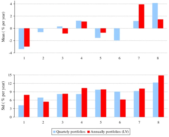
Table 1 presents a summary statistic for real returns and excess returns on the assets to be priced over the period 1977:1 to 2004:4. The average real return on the covered trading of foreign government bonds ranges from 1.77% to 2.60% a year, except for the Swiss bonds with 7.88%, while that of uncovered trading ranges from 2.72% to 5.14%. The real return on the S&P500 is 9.23% at an annual rate, while that of the 90-day T-bill is 1.78%, with a resulting excess return (equity premium) of 7.35%. As expected, real stock returns are much more volatile than the U.S. Treasury Bill return—annualized standard deviations of 16.64% and 1.61% respectively. Some of the foreign-currency portfolios in the Lustig and Verdelhan (2007) database have a negative real excess return but, in general, their volatilities seem to be modest, corroborating these same statistics for original annually re-balanced portfolios, as one can observe in Figure 2. In contrast, means and standard deviations of the Fama and French portfolios are quite high, reaching more than 17% and 29% respectively.
required to match the high equity Sharpe ratio of the U.S. Hence, the smoothness of aggregate consumption growth is the main reason behind the EPP. Since the higher the Sharpe ratio, the tighter the lower bound on the volatility of the pricing kernel, a natural question that arises is the following: may we regard this fact as evidence that a kernel that prices correctly the equity premium would also price correctly the forward premium? In this sense, our results can be useful to answer this question in an indirect way.
4.2 SDF Estimates
Before presenting the results for SDF estimates, we tested all returns used either in estimating SDF’s or in the testing procedures for the presence of a unit root in the auto-regressive polynomial.19 Because returns are prone to displaying heteroskedas-ticity, we used thePhillips and Perron(1988) unit-root test including an intercept in the test regression. For almost all cases we rejected the null of a unit root at the 5% level and rejected the null for all cases at the 10% level. We take this as evidence that all returns and the pricing kernels are well behaved.20
The first step in constructing M^∗ST
t , from the real returns on all traded U.S. stocks, is to choose the number of factors. Following Lehmann and Modest (1988), Connor and Korajczyk (1988), Tsay(2001) and most of the empirical literature, we took a pragmatic, informal, but useful view, examining the time plot of the eigenvalues ordered from the largest to the smallest. We are able to determine appropriately that five factors are needed to account for about a representative portion of the variation of our 464 stock returns, a choice (five factors) that is close to the one inConnor and Korajczyk (1993), who examined returns from stocks listed on the New York Stock Exchange and the American Stock Exchange. For the second SDF, with only three factors, more than 99% of the variation of the one hundred Fama-French portfolios is explained.
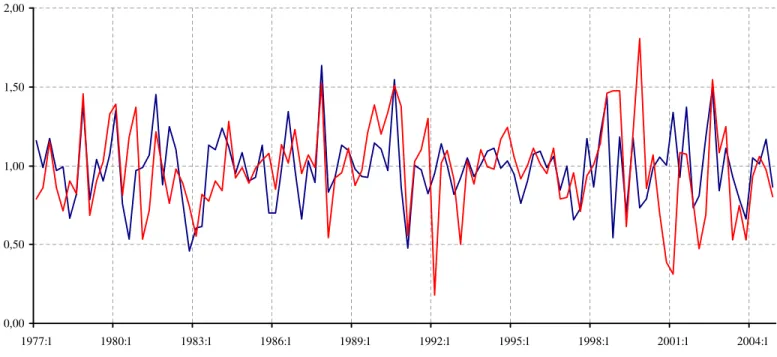
The estimates of M∗
t—M^
∗ST
t and M
∗F F
t —are plotted in Figure 1, which also include their summary statistics. Their means are slightly below unity. The pricing kernel extracted from the Fama-French portfolios is more volatile than the first one and the correlation coefficients between them is 0.357.
19
SeeHansen(1982) andOgaki(1992) for more details.
4.3 Pricing-Test Results
Tables 2 and 3 present results on the behavior of our return-based pricing kernels,
M∗ST
t and Mt∗F F—formed using only domestic U.S. returns—in pricing returns re-lated to the EPP and other domestic returns discussed in the literature. These are in-sample tests. Table 2 tests the system of orthogonality restrictions (30), accounting for the equity premium,RSPt+1−Rtb+1,and for the return on S&P500,RSPt+1. We use a constant as instrument as well as (D/P)t and (I/C)t. Table 3 presents pricing tests on the Fama-French benchmark portfolios using as instruments a constant and the Fama-French factors.
These in-sample tests show no evidence that pricing errors are relevant: at the 5% significance level, pricing errors are all statistically zero (individually or jointly) and the T×J statistics do not reject the null that weighted pricing errors are zero. Notice that pricing errors and the respective standard errors are multiplied by 100.
Tables 4, 5 and 6 present our main results, i.e., the results of out-of-sample pricing tests, whereM^∗ST
t and Mt∗F F are respectively used to price foreign assets related to the FPP and other foreign returns on dynamic portfolios discussed in the literature. Table 4 presents the results of tests for the system of orthogonality restrictions (25). There are two Euler equations: one with the excess return on uncovered over covered trade with foreign government bonds RU
t+1−RCt+1
, and one with the un-covered return, RUt+1. The instrument set includes a constant and the variable that generates the FPP in regression (10), (tFtj+1−Stj)/Stj, making the result of these tests very informative with regards to the FPP. At the 5% significance level, all individual pricing errors are statistically zero for all foreign currencies studied here. Wald-test results show no sign of joint significance for currency-pricing errors, with identical results for all the over-identifying restriction tests for currencies. Moreover, the size of the pricing errors is relatively modest, lower than unity with a mean value of 0,5%,
when trying to price returns and excess returns simultaneously.
In Table 5 we present joint tests of the FPP and of the EPP for Canada, Germany, Japan, Switzerland and the U.K. These pricing restrictions stack the Euler equations that characterize the EPP tested in Table 2 and those tested in Table 4, i.e., the system (28). The instrument set is the union of the sets previously considered: a constant, (tFtj+1 −S
j t)/S
j
levels, whereas joint Wald tests reject that all pricing errors are zero for Canada and Japan at these same levels. A way to reconcile this last set of results is to imagine that pricing errors are indeed correlated, perhaps strongly. If this is case, it is possible for individual tests not to reject the null while joint tests produce the opposite result.21
Table 6 presents pricing tests for the dynamicLustig and Verdelhan(2007) foreign currency portfolios, whenM∗F F
t is used in testing (29). The pricing error of portfolio 1 is significantly different from zero at the 5% level in out-of-sample tests. Portfolio 1 is the portfolio built with the lowest interest rate currencies relative to the U.S. T-bill. Due to rejection of Portfolio 1 in these pricing tests, joint Wald-tests also reject the group of portfolios 1 - 8. Further investigation on pricing errors confirms that mispricing comes indeed from Portfolio 1 alone. Once we remove it from the Lustig and Verdelhan set of portfolios, there is no evidence of mispricing at the 5% level. Despite that, Hansen(1982) T×J statistic is insignificant, which can be interpreted to mean that weighted pricing-errors on all portfolios are statistically zero.
The results in Tables 4, 5 and 6 show strong evidence that M^∗ST
t and M
∗F F
t are
able to account for most of the puzzling aspects in asset pricing, as the EPP and the FPP. Also, there is strong evidence that they price correctly all the dynamic Fama-French portfolios and all the Lustig and Verdelhan portfolios—with the exception of Portfolio1.
Here, we should stress that M^∗ST
t and M
∗F F
t were constructed using domestic asset returns alone. Therefore, these exercises are out-of-sample. Moreover, our results do not come from increased variance. Indeed, when using the multi-factor SDF estimate, the discounted return, i.e., scaled by M∗
, displayed lower variance than the undiscounted return. The high p-values found in this paper come from lower pricing errors, not higher variance.22
Table 7 displays the performance ofM^∗ST
t in predicting returns and excess returns on uncovered and covered trading of British, Canadian, German, Japanese and Swiss bonds. Table 8 presents the same result forM∗F F
t in predictingLustig and Verdelhan (2007)’s foreign currency portfolios.
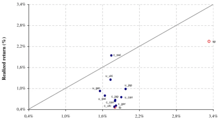
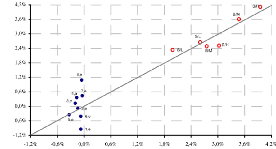
In Figures 3 and 4 we show predicted versus realized average return (to be precise,
21
Hansen (1982)’sJ-test does not reject the null beacuse it evaluates the quadratic form at the optimal level, using the identity matrix as a weighting factor. This, of course, does not take into account the cross-correlation of the pricing errors.
22
net return) and excess return for each pricing kernel. Pricing errors are measured by the distance to the 45-degree line (dotted line). The pricing kernels do a reasonable job in predicting excess returns on trading with foreign government bonds and on dynamic foreign currency portfolios. The main exceptions are the excess return on Swiss bonds and the two extreme portfolios of Lustig and Verdelhan, for which pricing errors are large.
As expected, in-sample forecasts are in general better than out of sample forecasts. Evidence toward this fact is found in Table 7, where we display the forecasting gains of using Mg∗
t: a global pricing kernel constructed by da Costa et al. (2008) from aggregate returns on stocks and government bonds for G7 countries and on Lustig and Verdelhan(2007)’s eight foreign dynamic currency portfolios. The gain in using such pricing kernel vis a visM^∗ST
t is about 20%. Based on results reported in Table 8, the out-of-sample forecast are quite reasonable, more so if we consider the high values for the excess returns on portfolios in question.
Finally, according to Hansen and Jagannathan (1997), ”[...] pricing errors may occur either because the model is viewed formally as an approximation, [...] or because the empirical counterpart to the theoretical stochastic discount factor is error ridden”. In this sense, we are able to show that M^∗ST
t , a SDF constructed to account only for domestic puzzles, not only does a good job in accounting for foreign market results, based on χ2 statistics, but, in fact, performs better than Mgt∗, according to the pricing error measure developed by these authors. The measures are 0.41 and 0.36, respectively.
Discussion Notwithstanding the rejection for one of the Lusting and Verdelhan
portfolios in pricing tests, and two joint rejections on Wald tests, the favorable out-of-sample tests results obtained in Tables 4 through 6 are in sharp contrast with those formerly obtained in log-linear tests of the FPP and the results obtained using consumption-based kernels. As argued above, this may suggest the inappropriateness of log linearizing the Euler equation or of the use of consumption-based pricing kernels. As in any empirical exercise, it is important to verify whether results are robust to changes in the environment used in testing. Here, we changed the conditioning set used through Tables 2 to 6 as well as the assets directly being tested in pricing. In both instances the basic results remain unchanged and are available upon request.
found when the ratiotFt+1/Stis used as an instrument and the theoretical restrictions tested were not rejected. This suggests that tFt+1/St has no predictive power for
M∗
t+1
Pt(1 +i∗t+1)
Pt+1
tFt+1−St+1
St
,
despite having predictive power for
Pt(1 +i∗t+1)
Pt+1
tFt+1−St+1
St
.
Hence, although the excess returns on uncovered over covered trading with for-eign bonds are predictable, “risk adjusted” excess returns are not. Another piece of evidence on this regard is the relative success in pricing Lustig and Verdelhan’s port-folios. We have shown that discounted excess return ofLustig and Verdelhan(2007)’s dynamic currency portfolios are zero, with the exception of one portfolio: the one with the lowest returns.
Another important aspect of our analysis is based on our theoretical discussion of log-linear approximations of the Euler equation. We point out to the inappropriate-ness of the log-linear approximations previously employed in testing theory. Hence, our empirical tests are robust to important sources of misspecification incurred by the previous literature: inappropriate log-linear approximation of the Euler equation for returns and inappropriate models for consumption-based kernels.
5
Conclusion
Previous research has cast doubt on whether a single asset pricing model was capable of correctly pricing the equity and the forward premium, which lead to the emergence of two separate literatures. We defy this position and propose a fresh look into the relationship between the Equity and the Forward Premium Puzzles.
the space of returns.
By working with a U.S. based version of SDF estimates, we were able to show that the factors contained in domestic (U.S.) market returns yield neither evidence of the EPP nor evidence of the FPP for most cases, corroborating the notion that these two puzzles are neither a consequence of any specificities of the domestic or the foreign markets, nor a consequence of a violation of the law of one price. Instead, they are but two instances of the poor performance of consumption-based pricing kernels in pricing assets in general.
Our starting point is the Asset Pricing Equation, coupled with the use of consistent estimators of the SDF mimicking portfolio. We first show that, our estimated return-based kernels constructed using domestic (U.S.) returns alone price correctly the equity premium, the 90-day T-bill and the Fama-French portfolios. When discounted by our pricing kernels, excess returns are shown to be orthogonal to past information that is usually known to forecast undiscounted excess returns. Based on these results, we go one step further and ask whether the EPP and the FPP are but two symptoms of the same illness—the inability of standard (and augmented) consumption-based pricing kernels to price asset returns or excess-returns. In our tests, we found that theex-ante forward premium is not a predictor of discounted excess returns, despite their being so for undiscounted excess returns.
These results invite the profession to concentrate the efforts on writing successful consumption models instead of wasting resources on trying to find specific details of foreign markets that would drive the systematic departure of the UIP characterizing the FPP. Given the tendency in the profession of generating new research agendas whenever a new empirical regularity that cannot be accounted for by our models is discovered, it is important to always ask whether these are distinct phenomena or if they are but two manifestations of a single problem.
We believe to have offered evidence that the answer to the question posed in the title of this paper is in the affirmative. A different and interesting issue is related to the provocative use of the term “risk adjusted” in the previous paragraphs. Should the forward premium be regarded as a reward for risk taking? If we take the covariance with M∗
t+1 as the relevant measure of risk, then our answer is yes. This position is
al. (2006) for whom the behavior of the SDF is equal to that of the intertemporal marginal rate of substitution for a model of preferences and/or market structure yet to be written. In this sense, we have provided grounds to believe that the striking similarity in the results found in trying to apply the CCAPM for the two markets is not accidental.
References
Araujo, Fabio and Jo˜ao V. Issler, “A Stochastic Discount Factor Approach to
Asset Pricing using Panel Data,” 2008. mimeo. Funda¸c˜ao Getulio Vargas. 11
Backus, David K., Silverio Foresi, and Chris I. Telmer, “Interpreting the
forward premium anomaly,” Canadian Journal of Economics, 1995, pp. 108–119. 9
Bai, Jushan, “Panel data models with interactive fixed effects,” 2005. Working
Paper: New York University. 15
Brandt, Michael W., John H. Cochrane, and Pedro Santa-Clara,
“Interna-tional risk sharing is better than you think, or exchange rates are too smooth,”
Journal of Monetary Economics, 2006, 53, 671–698. 30
Breeden, Douglas, “An intertemporal asset pricing model with stochastic
con-sumption and investment opportunities,”Journal of Financial Economics, 1979,7, 265–296. 5
Burnside, Craig, “The Cross-Section of Foreign Currency Risk Premia and
Con-sumption Growth Risk: A Comment,” Working paper 13129, NBER 2007. 3
, Martin Eichenbaum, Isaac Kleshchelski, and Sergio Rebelo, “The returns
to currency speculation,” Working paper 12489, NBER 2007. 3,5,6,9,10
Campbell, John Y. and Robert J. Shiller, “The dividend-price ratio and the
expectations of future dividends and discount factors,”Review of Financial Studies, 1988, 1, 195–228. 22
Chamberlain, Gary and Michael Rothschild, “Arbitrage, factor structure, and