Essays on the relationship between the equity and the forward premium puzzles

Escola de Pós-Graduação em Economia -- EPGE

Fundação Getulio Vargas

Essays on the relationship between the Equity and

the Forward Premium Puzzles

Tese submetida à Escola de Pós-Graduação em Economia da Fundação Getúlio

Vargas como requisito de obtenção do título de Doutor em Economia.

Aluno: Paulo Rogério Faustino Matos

Professor Orientador: Carlos Eugênio Ellery Lustosa da Costa

Escola de Pós-Graduação em Economia -- EPGE

Fundação Getulio Vargas

Essays on the Relationship between the Equity and

the Forward Premium Puzzles

Tese submetida à Escola de Pós-Graduação em Economia da Fundação Getúlio

Vargas como requisito de obtenção do título de Doutor em Economia.

Aluno: Paulo Rogério Faustino Matos

Banca Examinadora:

Carlos Eugênio Ellery Lustosa da Costa (Orientador, EPGE)

Caio Ibsen de Almeida (EPGE)

Marco Antônio Bonomo (EPGE)

Marcelo Fernandes (Queen Mary University of London)

Ricardo Dias de Oliveira Brito (Ibmec-SP)

Contents

Acknowledgements iv

List of Tables v

List of Figures vi

Introduction 1

Chapter 1 - The Forward- and the Equity-Premium Puzzles: Two Symptoms of the

Same Illness? 4

Chapter 2 - On the relative performance of consumption models in foreign and domestic

markets.* 50

Chapter 3 - Modeling foreign currency risk premiums with time-varying covariances

86

Acknowledgements

Agradeço,

A Deus pela iluminação e proteção,

À minha família pelo apoio incondicional e confiança,

À minha noiva e futura esposa, Cristiana, pelo amor e compreensão ao longo deste

período em que a privei de meu convívio,

Ao meu orientador, Carlos Eugênio, um incansável parceiro cuja contribuição foi

fundamental para a minha formação e para o desenvolvimento desta tese e

List of Tables

Chapter 1

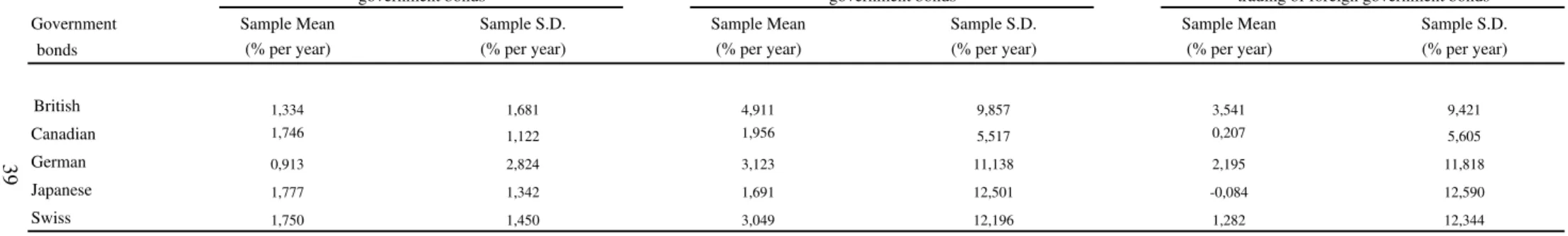
Table 1 – Data summary statistics 39

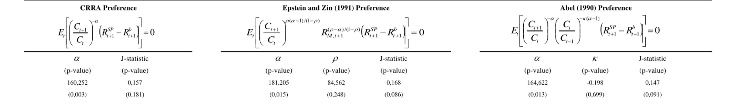
Table 2 – Testing overidentifying restrictions of consumption models 40

Table 3 – Equity-Premium Puzzle tests (single-equation) 42

Table 4 – Forward-Premium Puzzle tests (single-equation) 43

Table 5 – Forward-Premium Puzzle tests (single-equation) 44

Table 6 – Equity-Premium Puzzle tests (system) 45

Table 7 – Fama-French portfolios pricing testes (system) 45

Chapter 2

Table 1 – Data summary statistics 77

Table 2 – Testing CRRA preference 78

Table 3 – Testing Abel (1990)

catching up with the Joneses

preference 79

Table 4 – Testing Epstein and Zin (1989, 1991) preference 80

Table 5 – Testing a modified Campbell and Cochrane (1999)

habit formation

preference 81

Chapter 3

Table 1 – Data summary statistics 110

List of Figures

Chapter 1

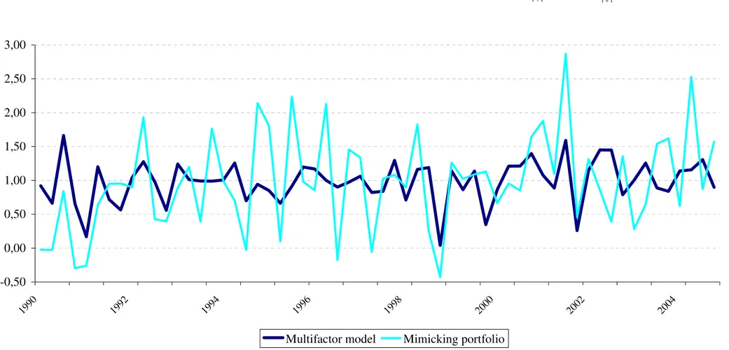
Figure 1 – Pricing kernels with US domestic financial market (1990:I – 2004:III) 41

Chapter 2

Figure 1 – Realized vs. fitted excess returns (taking into account the instrument

set IS1) 82

Figure 2 – Realized vs. fitted excess returns (taking into account the instrument

set IS2) 83

Chapter 3

INTRODUCTION

The Consumption Capital Asset Pricing Model— CCAPM— presented to the

profes-sion by the seminal works of Lucas (1978) and Breeden (1979) speci…es from an

equilib-rium relation the Stochastic Discount Factor— SDF— as the intertemporal marginal rate

of substitution for the representative agent, incorporating de…nitely the …nancial theory

to the theoretical framework developed by the economists of choice under uncertainty.

In its canonical version, the CCAPM de…nes the consumption growth as the SDF.

Although this speci…cation has been extensively used in …nance literature due to its

convenience, it really does not work well in practice, there being many evidences of its

incapability to account for stylized facts. The equity premium— EPP— and the forward

premium puzzles— FPP— are two of the most famous and reported empirical failures

of this consumption-based approach.

The EPP, commonly associated with the works of Hansen and Singleton (1983) and

Mehra and Prescott (1985), is how one calls the incapacity of consumption based asset

pricing models, with reasonable parameters for the representative agent’s preferences, to

explain the excess return of stock market with respect to the risk free bond in the United

States. The departure point of the puzzle is an attempt to …t the Euler equation of a

representative agent for the American economy, which has proven to be an elusive task.

The FPP, on the other hand, relates to the di¤erence between the forward rate and

the expected future value of the spot exchange rate in a world with rational expectations

and risk neutrality. Once more, this risk premium model fails when it is not able to

generate the conditional bias of the forward rates as predictors of future spot exchange

rates that characterizes the FPP.

Relaxing the risk neutrality hypothesis, The relevant question is whether a

theoret-ically sound economic model is able to provide a de…nition of risk capable of correctly

pricing the forward premium. In other words, although the two puzzles are similar with

regards to the incapacity of traditional models to account for the risk premiums involved

in these di¤erent markets, there is a non-shared characteristic: the predictability of

re-turns based on interest rate di¤erentials. It is possible that it was this speci…city that

lead researchers to adopt distinct agendas for investigating these puzzles. Engel (1996),

exchange rate changes has no counterpart in the literature on equity returns, general

equilibrium models are not likely to replicate this …nding, there being no grounds to

believe that the proposed solutions to puzzles in domestic …nancial markets can shed

light on the FPP.

More recently, some works intending to better understand the behavior of foreign

currency risk premiums have considered the possible relation between these puzzles, but

none of them has provided empirical evidences toward this direction.

In this sense, our research agenda consists in showing this strong relation between

these puzzles based on evidences that both empirical failures are related to the

incapac-ity of the canonical CCAPM to provide a high volatile intertemporal marginal rate of

substitution with reasonable values for the preferences parameters.

The …rst chapter (with João Victor Issler) has as a departure point that given free

portfolio formation and the law of one price is equivalent to the existence of a SDF

through Riesz representation theorem, which relies on less restrictive assumptions than

those ones used in the CCAPM. Using two di¤erent purely statistical methodologies we

extract time series for the SDF which are able to correctly price the excess market return

and also the excess returns that characterizes the FPP. Our results not only suggest that

both puzzles are interwined, but also that American domestic are "representative" in

the sense of characterizing a pricing kernel capable to price the foreign currency risk

premium.

Because we do not spell out a full speci…ed model it is hard to justify our calling the

covariance of returns with the SDF as a risk measure. In the second chapter, we take

the discussion of the previous chapter one step further by evaluating the performance of

di¤erent models in pricing excess returns for each market. Once again, our goal is not

to …nd a model that solves all the problems. Rather, our concern is to verify if the same

failures and successes attained by the CCAPM in its various forms in pricing the excess

returns of equity over short term risk-free bonds will be manifest in the case of forward

exchange markets. Our main …nding is that the same (however often unreasonable)

values for the parameters are estimated for all models in both markets.

In most cases, the rejections or otherwise of overidentifying restrictions occurs for the

two markets, suggesting that success and failure stories for the equity premium repeat

et al. (2006) that indicate a strong similarity between the behavior of excess returns in

the two markets when modeled as risk premiums, providing empirical grounds to believe

that the proposed preference-based solutions to puzzles in domestic …nancial markets

can certainly shed light on the Forward Premium Puzzle.

However, even though one can write a successful risk premium model, which has been

a surmountable task, there is a robust and uncomfortable empirical …nding typical of

the FPP that remains to be accommodated: domestic currency is expected to appreciate

when domestic nominal interest rates exceed foreign interest rates.

In this sense, the third chapter (with Fabrício Linhares) revisits these

counterintu-itive empirical …ndings working directly and only with the log-linearized Asset Pricing

Equation. We are able to derive an equation that describes the currency depreciation

movements based on a quite general framework and that has the conventional regression

used in most empirical studies related to FPP as a particular case, therefore, being useful

to identify the potential bias in the conventional regression due to a problem of omitted

variable. We adopt a novel three-stage approach, wishing to analyse if this bias would

be responsible for the disappointing …ndings reported in the literature. This chapter is

still in process and the results are partially well succeed. In some tests we are not able

to reject the null hypothesis that risk explains the FPP, while in other tests we reject

CHAPTER 1

The Forward- and the Equity-Premium Puzzles: Two Symptoms of the Same Illness?1

Abstract

In this paper we revisit the relationship between the equity and the forward premium

puzzles. We construct return-based stochastic discount factors using only American

do-mestic assets and check whether they price correctly the foreign currency risk premia.

We avoid log-linearizations by using moments restrictions associated with euler

equa-tions. Our pricing kernel accounts for both domestic and international markets stylized

facts that escape consumption based models. In particular, we fail to reject the null

hypothesis that the foreign currency risk premium has zero price when the instrument

is the own current value of the forward premium.

JEL Code: G12; G15. Keywords: Equity Premium Puzzle, Forward Premium Puzzle,

Return-based Pricing Kernel.

1. Introduction

The Forward Premium Puzzle – henceforth, FPP – is how one calls the systematic

departure from the intuitive proposition that the expected return to speculation in the

forward foreign exchange market should be zero, conditional on available information.

One of the most acknowledged puzzles in international …nance, the FPP was, in its

infancy, investigated by Mark (1985) within the framework of the consumption capital

asset pricing model – CCAPM. Perhaps, following Hansen and Singleton’s (1982, 1984)

earlier method, Mark used a non-linear GMM approach, which revealed the model’s

inability, in its canonical version, to account for its implicit over-identifying restrictions.

The results found by Mark are similar to the ones found by Hansen and Singleton with

respect to the equity premium, an idea carried forward by Mehra and Prescott (1985) who

went on to propose what they have labelled the Equity Premium Puzzle – henceforth,

EPP.

At …rst sight, it may seem surprising that such similar results were never properly

apart after the work of Mark. We list two alternative explanations. First, the failure of

the CCAPM was a great disappointment for the profession, since it meant the absence of

a fully speci…ed economic model that could price assets. Such unheartening …nding may

have lead to a momentary halt in research linking the equity- and the forward-premium

puzzles2_{. Second, the existence of a speci…city of the FPP with no parallel in the case of}

the EPP – the predictability of returns based on interest rate di¤erentials3 – may have

led many to believe that even if the CCAPM was capable of accounting for the equity

premium it would not solve the FPP; see Engel (1996).

Thinking deeper about these two puzzles, we are forced to conclude that proving

that they are related is currently an impossible task, since it requires the existence of a

consumption model generating a pricing kernel that properly prices assets, showing the

shortcomings of previous models. Because we do not have such a proper model today, we

cannot relate the EPP and the FPP within a CCAPM framework. This may explain why

relating these two puzzles was not tried before and why two distinct research agendas

involving them appeared over time.

As is well known, research regarding the FPP is mostly done within the scope of

international economics, like in Fama and Farber (1979), Hodrick (1981) and Lucas

(1982). It emphasizes international a¢ne term structure models and/or a microstructure

approach. Research involving the EPP has focused on adding state variables to standard

consumption-based pricing kernels to change its behavior; see Epstein and Zin (1989),

Constantinides and Du¢e (1996) and Campbell and Cochrane (1999).

In this paper we revisit the FPP and the EPP and ask whether they deserve two

distinct agendas, or whether they are but two symptoms of the same illness: the

in-capacity of existing consumption-based models to generate the implied behavior of a

pricing kernel that correctly prices asset returns.

Given the limitations on proving that the FPP and the EPP are related, we use an

indirect approach. If these two puzzles are solely a symptom of the inappropriateness

of existing consumption-based pricing kernels, then they will not be manifest when

ap-propriate pricing kernels are used. Suppose we …nd a single pricing kernel that is not

a function of consumption and is compatible with all regularities in domestic …nancial

markets not accounted for by current consumption-based kernels. At the same time,

have good reason to believe that we should not disperse our research e¤ort on two

com-pletely di¤erent agendas, but rather concentrate on a single one focused on rethinking

consumption-based pricing kernels4 _{– the common suspect for the two puzzles.}

A crucial issue of our approach is to …nd what anappropriate pricing kernel is in this context. Hansen and Jagganathan (1991) have lead the profession towards return-based

kernels instead of consumption-based kernels; see also Connor and Korajczyk (1986),

Chamberlain and Rothschild (1983), and Bai (2005). The idea is to combine statistical

methods with economic theory – the Asset Pricing Equation – to devise pricing-kernel

estimates as the unique projection of a stochastic discount factor – henceforth, SDF – on

the space of returns: the SDF mimicking portfolio. The latter can be estimated without

any assumptions on a functional form for preferences, despite having a strong footing on

theory as a consequence of the use of the Asset Pricing Equation.

One way to rationalize the SDF mimicking portfolio is to realize that it is the

projec-tion of a proper consumpprojec-tion model (yet to be written) on the space of payo¤s. Thus, the

pricing properties of this projection are no worse than those of the proper model – a key

insight of Hansen and Jagganathan. An advantage of concentrating on the projection is

that we can approximate it arbitrarily well in-sample using statistical methods and asset

returns alone. Therefore, using such projection not only circumvents the inexistence of a

proper consumption model but is also guaranteed not to underperform such ideal model.

Bearing in mind our stated goal, we extract a time series for the pricing kernel that

does not depend on preferences or on consumption data. Two techniques are considered

in this paper to estimate the SDF mimicking portfolio: i) Hansen and Jagganathan’s

mimicking portfolio, which is the projection of any stochastic discount factor on the

space of returns and ii) the unconditional linear multifactor model, which is perhaps the

dominant model in discrete-time empirical work in Finance.

As noted by Cochrane (2001), SDF estimates are just functions of data. Pricing

correctly a speci…c group of assets can be achieved by building non-parsimonious SDF

estimates, i.e., SDF estimates that price arbitrarily well that group of assets in-sample

but not necessarily assets outside that group.5 _{In order to avoid this critique, we}

con-struct SDF mimicking portfolio estimates using domestic (U.S.) returns alone – on the

200 most traded stocks in the NYSE, extracted from the CRSP database.

Then, the behavior of its projection on the space of domestic-asset returns would have to

coincide with that of an SDF mimicking portfolio built from these same assets. We then

use this domestic SDF projection to price the forward premium. Tests are implemented

for four countries within the G7 group, besides Switzerland, for which there exists a

relatively long-span data for spot and future foreign exchange markets. Here, our tests

show their out-of-sample character, avoiding Cochrane’s critique.

Our tests make intensive use of the Asset Pricing Equation. They are all based on

euler equations, exploiting theoretical lack of correlation between discounted risk premia

and variables in the conditioning set, or between discounted returns and their respective

theoretical means, i.e., we employdiscounted scaled excess-returns and discounted scaled returns in testing. We investigate whether discounted risk premia have mean zero or

whether discounted returns have a mean of unity.

Our results are clear cut: return-based pricing kernels using U.S. assets alone account

for domestic stylized facts, pricing correctly the equity premium for the U.S. economy –

which shows no signs of the EPP – and also pricing most of the Fama-French benchmark

factor returns. At the same time, these same pricing-kernel estimates show no signs

of the FPP in pricing the expected return to speculation in forward foreign-exchange

markets for the widest group possible of developed countries with a long enough span of

future exchange-rate data (Canada, Germany, Japan, Switzerland and the U.K.). This

evidence raises the question of whether the FPP and the EPP are two symptoms of the

same illness.

We summarize our empirical results as follows. First, the null of zero discounted

excess returns on equities is not rejected even when potentially interesting forecasting

variables are used as instruments. Second, for most countries, the moment restrictions

associated with the euler equations (Asset Pricing Equations) are not rejected for excess

returns and returns on operations with foreign assets for any of the instruments used.

This includes the own current value of the forward premium, which shows no signs of

predictability of the expected return to speculation, contradicting one of the de…ning

features of the FPP. Only in the case of British bonds the results are, in some sense,

con‡icting. In some occasions, we reject the null hypothesis that the foreign currency

risk premium has zero price.

research agendas on the EPP and the FPP. Although we cannot claim that a consumption

model that did account for the behavior of the equity premium would also price correctly

the forward premium, we can claim that its projection on the space of domestic returns

would.6 In our view, this is as far as one can go today in showing that these two puzzles

are related.

As argued above, we search not for a consumption model of the SDF, but simply

for a procedure that identi…es the SDF mimicking portfolio circumventing the fact that

we still lack a good model for pricing risk or risk premia. Employing SDF mimicking

portfolio estimates allows to test directly the pricing of risk or risk premia by using the

theoretical restrictions associated with the Asset Pricing Equation. In our context, there

is neither the need to specify a full model for preferences (consumption SDF) nor the

need to perform a log-linearization of the Asset Pricing Equation in pricing tests. In

that sense, we are able to isolate possible causes for rejection of theory (EPP and FPP)

not isolated by the previous literature.

The remainder of the paper is organized as follows. Section 2 gives an account of the

literature that tries to explain the FPP and is related to our current e¤ort. Section 3

discusses the techniques used to estimate the SDF and the pricing tests are implemented

in this paper. Section 4 presents the empirical results obtained in this paper. Concluding

remarks are o¤ered in Section 5.

2. A Critical Literature Review

Most studies7 _{report the existence of the FPP through the …nding that b}

1 is

signi…-cantly smaller than zero when running the regression,

st+1 st= 0+ 1(tft+1 st) +ut+1, (1)

where st is the log of the exchange rate at time t, tft+1 is the log of time t forward

exchange rate contract and ut+1 is the regression error.8 Notwithstanding the possible

e¤ect of Jensen inequality terms, testing the uncovered interest rate parity (UIP) is

equivalent to testing the null 1 = 1 and 0 = 0, along with the uncorrelatedness of

residuals from the estimated regression.

Although the null is rejected in almost all studies, it should be noted that 1 not

irrationality and, per se, does not imply the existence of a ‘puzzle’ since the uncovered parity needs only to hold exactly in a world of risk-neutral agents, or if the return

on currency speculation is not risky. The probable reason why these …ndings came to

be called a puzzle was the magnitude of the discrepancy from the null: according to

Froot (1990), the average value of ^1 is 0:88 for over 75 published estimates across

various exchange rates and time periods. This implies an expected domestic currency

appreciation when domestic nominal interest rates exceed foreign interest rates, contrary

to what is needed for the UIP to hold.

Log-linear regressions such as (1) have a long tradition in economics. As is well

known, getting to (1) from …rst principles requires stringent assumptions, something

that is usually overlooked when hypothesis testing is later performed using it. Next, we

shall make explicit how strong the assumptions that underlie the null tested in (1) are.

Our departing point is the Pricing Equation,

1 =E_{t[Mt+1Ri;t+1] 8i= 1;2; ; N: (2)}

whereRi;t+1 is the return of assetiandMt+1 is the pricing kernel or stochastic discount

factor, SDF (e.g. Hansen and Jagganathan (1991)), a random variable that discount

payo¤s in such a way that their price is simply the discounted expected value.

Given free portfolio formation, the law of one price – the fact that two assets with the

same payo¤ in all states of nature must have the same price – is su¢cient to guarantee,

through Riesz representation theorem, the existence of a SDF,Mt+1. Log linearizing (2)

makes it is possible to justify regression (1), but not without unduly strong assumptions

on the behavior of discounted returns.

Gomes and Issler (2007) criticize the empirical use of the log-linear approximation of

the Pricing Equation (2) leading to (1). First, is the usual criticism that any hypothesis

test using results of a log-linear regression is a joint test which includes the validity of

the log-linearization being performed, i.e., includes an auxiliary hypothesis in testing.

Therefore, rejection can happen if the null is true but the log-linearization is

inappropri-ate. Second, they show that it is very hard to …nd appropriate instruments in estimating

log-linear regressions such as (1), since, by construction, lagged variables are correlated

with the error term.

exponential function aroundx, with incrementh,

ex+h=ex+hex+h

2_ex+ (h)h

2 ; with (h) :R!(0;1). (3) For a generic function, ( )depends on bothxandh, but not for the exponential function. Indeed, dividing (3) byex_{, we get}

eh = 1 +h+h 2_e (h)h

2 ; (4)

showing that ( ) depends only on h.9 _{To connect (4) with the Pricing Equation (2),}

we assume MtRi;t >0 and let h= ln(MtRi;t)to obtain10

MtRi;t = 1 + ln(MtRi;t) +zi;t; (5)

where the higher-order term of the expansion is

zi;t 1

2 [ln(MtRi;t)]

2_e (ln(MtRi;t)) ln(MtRi;t)_.

It is important to stress that (5) is not an approximation but an exact relationship.

Also, zi;t 0. Taking the conditional expectation of both sides of (5), using past

information, denoted byE_{t 1( ), imposing the Pricing Equation, and rearranging terms,} gives:

E_{t 1fMtRi;tg = 1 +}E_{t 1fln(MtRi;t)g+}E_{t 1(zi;t), or, (6)}

E_{t 1(zi;t) =} E_{t 1fln(MtRi;t)g: (7)}

Equation (7) shows that behavior of the conditional expectation of the higher-order

term depends only on that of E_{t 1fln(MtRi;t)g. Therefore, in general, it depends on} lagged values of ln(MtRi;t) and on powers of these lagged values. This will turn out

to a major problem when estimating (1). To see it, denote by "i;t = ln(MtRi;t)

E_{t 1fln(MtRi;t)g the innovation ofln(MtRi;t):Let} R_{t (R1;t; R2;t; :::; RN;t)}0 _and "_t ("1;t; "2;t; :::; "N;t)0 stack respectively the returnsRi;t and the forecast errors "i;t. From

the de…nition of "_t we have:

ln(MtRt) =Et 1fln(MtRt)g+"_t: (8)

Denoting r_{t= ln (}R_{t), with elementsri;t, and mt= ln (Mt) in (8), and using (7) we get}

Starting from (69), the covered, RC, and the uncovered return, RU, on foreign gov-ernment bonds trade are, respectively,

RC_t+1 = tFt+1(1 +it+1)Pt

StPt+1

and RU_t+1 = St+1(1 +it+1)Pt

StPt+1

, (10)

where tFt+1 and St are the forward and spot prices of foreign currency in terms of

domestic currency,Pt is the dollar price level andit+1 represents nominal net return on

a foreign asset in terms of the foreign investor’s preferences.

Using a forward version of (69) on both assets, and combining results, yields:

st+1 st= (tft+1 st) [Et(zU;t+1) Et(zC;t+1)] +"U;t+1 "C;t+1; (11)

where the indexiinE_{t(zi;t+1)and "i;t+1 in (69) is substituted by eitherC orU,} respec-tively for the covered and the uncovered return on trading foreign government bonds.

Under 1= 1 and 0= 0 in (1), taking into account (11), allows concluding that:

ut+1= [Et(zU;t+1) Et(zC;t+1)] +"U;t+1 "C;t+1.

Hence, by construction, the error term ut+1 is serially correlated because it is a

function of current and lagged values of observables.11 However, in most empirical

studies, lagged observables are used as instruments to estimate (1) and test the null

that 1 = 1, and 0 = 0. In that context, estimates of 1 are biased and inconsistent,

which may explain the …nding that the average value of_c1 is 0:88for over75published

estimates across various exchange rates and time periods. As far as we know, this is the

…rst instance where FPP results are criticized in this fashion.

Because our goal is to relate the two puzzles, it is important to rephrase the FPP

in the same language as the EPP. Recalling that rational expectations alone does not

restrict the behavior of forward rates, since it is always possible to include a risk-premium

term that would reconcile the time series behavior of the involved data, e.g., Fama (1984),

the rejection of the null that 1 = 0, in favor of 1 <0, only represents a true puzzle if

reasonable risk measures cannot explain the empirical regularities of the data.

Here is where an asset-pricing approach may help, which is our starting point. The

relevant question is whether a theoretically sound economic model is able to provide

a de…nition of risk capable of correctly pricing the forward premium.12 _{The natural}

candidate for a theoretically sound model for pricing risk is the CCAPM of Lucas (1978)

Assuming that the economy has an in…nitely lived representative consumer, whose

preferences are representable by a von Neumann-Morgenstern utility function u( ), the …rst order conditions for his(ers) optimal portfolio choice yields

1 = E_t u

0

(Ct+1) u0_(C

t)

Ri;t+1 8i; (12)

and, consequently,

0 =E_t u

0

(Ct+1) u0_(C

t)

(Ri;t+1 Rj;t+1) 8i; j; (13)

where 2 (0;1) is the discount factor in the representative agent’s utility function,

Ri;t+1 and Rj;t+1 are, respectively, the real gross return on assets iand j at time t+ 1

and,Ctis aggregate consumption at timet:In other words, under the CCAPM,Mt+1 = u0

(Ct+1)=u0(Ct):

Let the standing representative agent be a U.S. investor who can freely trade domestic

and foreign assets.13 De…ne the covered and the uncovered return on trading foreign

government bonds as in (10) and substituteRC forRi and RU forRj in (12) to get

0 =E_t u

0

(Ct+1) u0_(C

t)

Pt(1 +it+1)[tFt+1 St+1] StPt+1

. (14)

Assuming that preferences exhibit constant relative risk aversion, Mark (1985)

esti-mated the parameter inu(C) =C1 (1 ) 1, applying Hansen’s (1982) Generalized Method of Moments (GMM) to (14), reporting an estimated coe¢cient of relative risk

aversion, _b, above 40. He then tested the over-identifying restrictions to assess the va-lidity of the model, rejecting them when the forward premium and its lags are used as

instruments. Similar results were reported later by Modjtahedi (1991). Using a

di¤er-ent, larger data set, Hodrick (1989) reported estimated values of_b above60, but did not reject the over-identifying restrictions, while Engel (1996) reported some estimated b’s in excess of 100. A more recent attempt to use euler equations to account for the FPP is Lustig and Verdelhan (2006 a), where risk aversion in excess of 100is needed to price the forward premium on portfolios of foreign currency.

Are we to be surprised with these …ndings? If we recall that the EPP is identi…ed

with the failure of consumption-based kernels to explain the excess return of equity over

risk-free short term bonds –Ri;t+1 = (1 +iSPt+1)Pt=Pt+1 and Rj;t+1 = (1 +ibt+1)Pt=Pt+1,

expect these same consumption-based models not to generate the FPP? Indeed, we

should expect the opposite.

The inexistence of a widely accepted model to account for risk is partly to blame

for the separation of the research agendas involving the two puzzles. There is, however,

an additional reason. Another characteristic of the FPP may have played a role in

the separation of these two research agendas: the predictability of returns on currency

speculation. Because _c1 < 0 and signi…cant, given that the auto-correlation of risk

premium is very persistent, interest-rate di¤erentials predict excess returns. Although

predictability in equity markets has by now been extensively documented, it was not

viewed as a de…ning feature of the EPP, back then. It was, however, a de…ning feature

of the FPP, which has lead Engel (1996, p. 155), for example, to write: “International

economists face not only the problem that a high degree of risk aversion is needed to

account for estimated values of [the risk premium demanded by a rational agent]. There

is also the question of why the forward premium is such a good predictor ofst+1 tft+1:

There is no evidence that the proposed solutions to the puzzles in domestic …nancial

markets can shed light on this problem.”

Predictability is now acknowledged to be present in domestic markets as well, in the

context of the equity premium. Dividend-to-price ratio, and other variables are capable

of predicting returns, which means that, once again, we should be suspicious that the

same underlying forces may account for asset behavior in both markets.

Before describing our strategy it is important to draw attention to the fact that

pricing excess returns is crucial, but should not be the sole goal of asset-pricing theory.

Returns, and not only excess returns need to be priced, and accomplishing both is a

much harder task. To make the point as stark as possible, let us get back to (12). When

we substitute RC _forR

i and RU forRj;we get

1 =E_t u

0

(Ct+1) u0_(C

t)

tFt+1(1 +it+1)Pt StPt+1

and 1 =E_t u

0

(Ct+1) u0_(C

t)

St+1(1 +it+1)Pt StPt+1

.

(15)

It turns out that in the canonical model, e.g., Hansen and Singleton (1982, 1983, 1984),

the parameter of risk aversion is the inverse of the intertemporal elasticity of substitution,

meaning that if one wants to accept a high risk aversion, one generates implausibly high

Accordingly, if one wants to identify the structural parameter , in an econometric

sense, one cannot resort to direct estimation of excess returns (e.g., 14), but rather to

joint estimation of the two euler equations for returns (e.g., 15), or to any linear rotation

of them. It is, therefore, important to make a distinction between studies that test

the over-identifying restrictions jointly implied by returns and those that test the ones

implied by excess returns. For the latter no-rejection may be consistent with any value for , including inadmissible ones.15

In our view, a successful consumption-based model must account for asset prices

everywhere (domestically and abroad), as well as price returns, excess returns, and many

new facts recently evidenced in the extensive empirical research that has been in a great

deal sparked by the theoretical developments of the late seventies - see, for example,

Cochrane (2006).

3. Our Strategy

The stated purpose of this paper is to relate the EPP and the FPP. The fact that, as of

this moment, no satisfactory consumption-based model derived from the primitives of the

economy can account for asset behavior in either market is a hint that it is generating

the two puzzles. We argue here in favor of an indirect approach. We do not need a

proper consumption model for the pricing kernel to link the two puzzles. All we need

is a strategy to extract a proper pricing kernel from return data, showing that it prices

both the domestic and the foreign-exchange returns and excess returns. This isolates

current consumption-based kernels as the most likely culprits for mispricing these two

markets. Of course, a …nal proof that these puzzles are linked in this fashion can only be

obtained when we …nally have a proper consumption-based model to price assets. That

will explain why current models fail, something we cannot do here.

Following Harrison and Kreps (1979) Hansen and Richard (1987), and Hansen and

Jagganathan (1991), we write the system of asset-pricing equations,

1 =E_{t[Mt+1Ri;t+1]; 8i= 1;2; ; N, (16)}

leading to

We combine statistical methods with these Asset Pricing Equations to devise

pricing-kernel estimates as projections of SDF’s on the space of returns, i.e., the SDF mimicking

portfolio, which is unique even under incomplete markets. We denote the latter by

M_t+1. These pricing kernels do not depend on any assumptions about a functional form for preferences, but solely on returns. In this sense, these methods are preference free,

despite the fact that they have a strong footing on theory as a consequence of the use of

the Asset Pricing Equation.

Our exercise consists in exploring a large cross-section of U.S. time-series stock returns

to construct return-based pricing kernel estimates satisfying the Pricing Equation (16) for

that group of assets. Then, we take these SDF estimates and use them to price assets not

used in constructing them. Therefore, we perform a genuine out-of-sample forecasting

exercise using SDF mimicking portfolio estimates, avoiding in-sample over-…tting.

We cannot overstress the importance of out-of-sample forecasting for our purposes.

Our main point in this paper is to show that the forward- and the equity-premium

puzzle are intertwined. Under the law of one price, an SDF exists that prices all assets,

necessarily. Thus, an in-sample exercise would only provide evidence that the

forward-premium puzzle is not simply a consequence of violations of the law of one price. We aim

at showing more: a SDF can be constructed using only domestic assets, i.e., using the

same source of information that guides research regarding the equity premium puzzle,

and still price foreign assets. It is our view that this SDF is to capture the growth of the

marginal utility of consumption in a model yet to be written.16

The main rationale for our methodological choice is the fact that, however successful,

a consumption-based model will not perform better in pricing tests than its related

mimicking portfolio. This is the main trust of Hansen and Jagganathan (1991). The

mimicking portfolio, thus, represents an upper bound on the pricing capability of any

model. Given our purposes an alternative approach would be to try and relate the

EPP and the FPP using a volatile consumption kernel constructed with high aversion

values. The trouble with this approach is that the work by Hansen and Singleton (1982,

1983, 1984) generated a consensus that the over-identifying restrictions of traditional

consumption models are often rejected when used to price not only excess returns but

also returns, i.e., when both the discount factor and the risk-aversion coe¢cient are

present in our data set as well.

Before moving on to the description of our methodology it is worth mentioning that,

in dispensing with consumption data, our paper parallels those of Hansen and Hodrick

(1983), Hodrick and Srivastava (1984), Cumby (1988), Huang (1989), and Lewis (1990),

all of which implemented latent variable models that avoid the need for specifying a

model for the pricing kernel by treating the return on a benchmark portfolio as a latent

variable. 17 _{Also related is Korajczyk and Viallet (1992). Applying the arbitrage pricing}

theory – APT – to a large set of assets from many countries, they test whether including

the factors as the prices of risk reduces the predictive power of the forward premium.

They do not perform any out-of-sample exercises and do not try to relate the two puzzles.

Finally, Backus et al. (1995) ask whether a pricing kernel can be found that satis…es,

at the same time, log-linearized versions of

0 = E_{t Mt+1}Pt(1 +it+1)[tFt+1 St+1]

StPt+1

and, (18)

Rf_t+1 = 1 E_t(M

t+1)

; (19)

whereRf_t+1is the risk-free rate of return. The nature of the question we implicitly answer is similar to the one posed by Backus et al. (1995), albeit adding a pricing test of the

excess return on equity over risk free short term bonds in the U.S.18

3.1. Econometric Tests

Assume that we are able to approximate well enough a time series for the pricing

kernel, M_t+1. Next, we show how to use this approximation to implement direct pricing tests for the forward and the equity-premium, in an euler equation framework. In Section

we discuss how to construct this time series forM_t+1 using asset-return information.

3.1.1. Pricing Test

In the context of the SDF mimicking portfolio, euler equations (16) and (17) must

directly test the validity of these euler equations using return data alone: the estimators

ofM_t are a function of return data and returns are also used to verify the Asset Pricing Equation. In this case, we do not have to perform log-linear approximations of these

euler equations, nor do we have to impose the stringent restrictions that returns are

log-Normal and Homoskedastic to test theory. Because we want our tests to beout-of-sample

the returns used to construct the estimates of M_t will not be the ones used directly in the euler equations when testing theory.

Consider zt to be a vector of instrumental variables, which are all observed up to

timet, therefore measurable with respect to E_{t( ). Employingscaled returns and scaled}

excess-returns – de…ned as Ri;t+1 zt and (Ri;t+1 Rj;t+1) zt, respectively – we are

able to test the conditional moment restrictions associated with the euler equations

and consequently to derive the implications from the presence of information. This is

particularly important for the FPP, since, when the CCAPM is employed, the

over-identifying restriction associated with having the own current forward premium as an

instrument is usually rejected: a manifestation of its predictive power.

Multiply

0 = E_{t M}

t+1

Pt(1 +it+1)[tFt+1 St+1] StPt+1

, and, (20)

1 = E_{t Mt+1}St+1(1 +it+1)Pt

StPt+1

(21)

by ztand apply the Law-of-Iterated Expectations to get, respectively,

0 = E _Mt+1Pt(1 +it+1)[tFt+1 St+1]

StPt+1

zt , and, (22)

0 = E _M

t+1

St+1(1 +it+1)Pt StPt+1

1 zt (23)

Equations (22) and (23) form a system of orthogonality restrictions that can be used

to assess the pricing behavior of estimates ofM_t+1 with respect to the components of the forward premium or any linear rotation of them. Equations in the system can be tested

separately or jointly. In testing, we employ a generalized method-of-moment (GMM)

parameters ₁ and ₂ in:

0 = E _M

t+1

Pt(1 +it+1)[tFt+1 St+1]

StPt+1 1

zt , and, (24)

0 = E _M

t+1

St+1(1 +it+1)Pt StPt+1

(1 ₂) zt (25)

We assume that there are enough elements in the vector zt for 1 and 2 to be over

identi…ed. In order for (22) and (23) to hold, we must have ₁= 0 and ₂ = 0, and the over-identifying restriction T J test in Hansen (1982) should not reject them. This

constitutes the econometric testing procedure implemented in this paper to examine

whether the FPP holds when return-based pricing kernels are used.

A similar procedure can be implemented for the domestic market equations, in order

to investigate domestic stylized facts that escape consumption based models. To analyze

the EPP, the system of conditional moment restrictions is given by:

0 = E

("

M_t+1(i SP

t+1 ibt+1)Pt

Pt+1 1

#

zt

)

, and (26)

0 = E

("

M_t+1(1 +i SP t+1)Pt Pt+1

(1 ₂)

#

zt

)

; (27)

where iSP_t+1 and ib_t+1 are respectively the returns on the S&P500 and on a U.S. govern-ment short-term bond, and we also test whether ₁ = 0 and ₂ = 0, and check the appropriateness of the over-identifying restrictions using Hansen’sT J test19.

Beyond the high equity Sharp ratio or the reported power of the dividend-price ratio

to forecast stock-market returns, the pattern of cross-sectional returns of assets exhibit

some “puzzling aspects” as the “size” and the “value” e¤ects – e.g. Fama and French

(1996) and Cochrane (2006) –, i.e., the fact that small stocks and of stocks with low

market values relative to book values tend to have higher average returns than other

stocks.

We follow Fama and French (1993) in using our pricing kernels to try and account for

their stock-market factors; zero-cost portfolios which are able to summarize these e¤ects,

moment restrictions is given by:

0 = E _M

t+1(Rm Rf)t+1 1 zt , (28)

0 = E _M

t+1HM Lt+1 2 zt and (29)

0 = E _M

t+1SM Bt+1 3 zt ; (30)

where Rm Rf, the excess return on the market, is the value-weighted return on all

NYSE, AMEX, and NASDAQ stocks minus the one-month Treasury bill rate, HM L

(High Minus Low) is the average return on two value portfolios minus the average return

on two growth portfolios andSM B(Small Minus Big) is the average return on three small

portfolios minus the average return on three big portfolios.20 We, again, test ₁ = 0;

2 = 0 and 3 = 0, and check the appropriateness of the over-identifying restrictions

using Hansen’s T J test.

It worth recalling that we employ an euler-equation framework, something that was

missing in the forward-premium literature after Mark (1985). Since the two puzzles

are manifest in logs and in levels, by working directly with the Pricing Equation we

avoid imposing stringent auxiliary restrictions in hypothesis testing, while keeping the

possibility of testing the conditional moments through the use of lagged instruments

along the lines of Hansen and Singleton (1982 and 1984) and Mark. We hope to have

convinced our readers that the log-linearization of the euler equation is an unnecessary

and dangerous detour. Any criticism arising from the use of the log-linear approximation

is avoided here.

An important feature of our testing procedure is its out-of-sample character. To

preserve the temporal structure of the euler equations, we perform out-of-sample tests

in the cross-sectional dimension, i.e., the returns used in estimating M_t+1 exclude the return of the assets appearing directly in our main tests. Therefore, there is no reason

for the Asset Pricing Equation to hold for the assets not used in estimating M_t+1.

3.1.2. Instruments

There seems to be a consensus in the return forecasting literature about the rejection

of the time-invariant excess returns hypothesis. However, the question of which variables

a representative set of forecasting instruments plays certainly an important role and

highlights the relevance of the conditional tests.

Taking into account the fact that expected returns and business cycles are correlated,

as documented in Fama and French (1989), for both domestic and international markets,

we use the following macroeconomic variables: real consumption instantaneous growth

rates, real GDP instantaneous growth rates, and the consumption-GDP ratio. However,

since in our exercise, the forecasting variables, the pricing kernels, and the excess returns,

are all based on market prices, we also include speci…c …nancial variables as instruments,

carefully choosing them based on their forecasting potential.

Regarding the FPP, besides using as instruments the past values for the covered and

uncovered returns on trading of the respective foreign government bond, we also use the

current value of the forward premium, since the well documented predictability power

of this variable is a de…ning feature of this puzzle.

For the Fama and French (1993) portfolios and the EPP, we use lagged values of

the returns on relevant assets as instruments, since one should not omit the possibility

that returns could be predictable from past returns for any …nancial market. Finally, for

the EPP we still use the dividend-price ratio, following Campbell and Shiller (1988) and

Fama and French (1988), who show evidences of the good performance of this variable

as a predictor of stock-market returns.

3.2. Return-Based Pricing Kernels and the SDF Mimicking Portfolio

The basic idea behind estimating return-based pricing kernels with asymptotic

tech-niques is that asset prices (or returns) convey information about the intertemporal

mar-ginal rate of substitution in consumption. If the Asset Pricing Equation holds, all returns

must have a common factor that can be removed by subtracting any two returns. A

com-mon factor is the SDF mimicking portfolioM_t+1. Because every asset return contains “a piece” ofM_t+1, if we combine a large enough number of returns, the average idiosyncratic component of returns will vanish in limit. Then, if we choose our weights properly, we

may end up with the common component of returns, i.e., the SDF mimicking portfolio.

Although the existence of a strictly positive SDF can be proved under no arbitrage,

uniqueness of the SDF is harder to obtain, since under incomplete markets there is, in

written as Mt+1 =Mt+1+ t+1 for some t+1 obeying Et[ t+1Ri;t+1] = 0 8i. Since the

economic environment we deal with is that of incomplete markets, it only makes sense to

devise econometric techniques to estimate the unique SDF mimicking portfolio – M_t+1. There are two basic techniques employed here to estimate M_t+1. The …rst one uses principal-component and factor analyses. It can be traced back to the work of Ross

(1976), developed further by Chamberlain and Rothschild (1983), and Connor and

Ko-rajczyk (1986, 1993). A recent additional reference is Bai (2005). This method is

as-ymptotic: eitherN ! 1orN; T ! 1, relying on weak law-of-large-numbers to provide consistent estimators of the SDF mimicking portfolio – the unique systematic portion of

asset returns. An alternative to this asymptotic method is to use a method-of-moment

approach, constructing algebraically the unique projection of any SDF on the space of

returns. This can be achieved through the following linear combination of traded returns:

M_t+1 10 E₍R_t+1R0 t+1)

1_R t+1;

where1_andR_{t+1areN 1vectors of ones and of traded returns respectively. This}

tech-nique was proposed by Hansen and Jagganathan (1991) to estimate the SDF mimicking

portfolio using the Pricing Equation. For sake of completeness, we present a summary

account of these the …rst method in section , as well as a more complete description of

both of them in the Appendix.

3.2.1. Multifactor Models

Factor models summarize the systematic variation of the N elements of the vector

R_{t = (R1;t; R2;t; :::; RN;t)}0 _{using a reduced number of K factors, K < N. Consider a} K-factor model inRi;t:

Ri;t =ai+ K

X

k=1

i;kfk;t+ it; (31)

where fk;t are zero-mean pervasive factors and, as is usual in factor analysis and

plim

N!1

1

N N

X

i=1

i;t = 0:

Denote by _r = E₍R_tR0

t) E(Rt)E(R0t) the variance-covariance matrix of returns.

maximal variance subject to the normalization that has unit norm, i.e., 0

= 1. Subsequent principal components are identi…ed if they are all orthogonal to the previous

ones and are subject to the same normalization. The …rst K principal components of

R_{t are consistent estimates of thefk;t’s. Factor loadings can be estimated consistently}

by simple OLS regressions of the form (31).

It is straightforward to connect principal-component and factor analyses with the

Pricing Equation, delivering a consistent estimator for M_t. Given estimates ofai, i;k,

and fk;t in (31), one can write their respective expected-beta return expression:

E_{(Ri) = +}

K

X

k=1

i;k k; i= 1;2; :::; N

where k is interpreted as the price of thek-th risk factor. The fact that the zero-mean

factorsf f~ E_{( ~f) are such thatf}~_{are returns with unitary price allows us to measure} the coe¢cients directly by

=E_{( ~f)}

and consequently to estimate only via a cross-sectional regression21. Given these

coe¢cients, one can easily get an estimate of M_t;

g

M_t a+ K

X

k=1 bkfk;t

where (a; b) is related to( ; ) through

a 1 and b cov(f f0

) 1 ;

It is easy then to see the equivalence between the beta pricing model and the linear

model for the SDF. More, it is immediate that

E₍g_M

tRi;t) = 1; i= 1;2; :::; N:

The number of factors used in the empirical analysis is an important issue. We

expectK to be rather small. We followed Lehmann and Modest (1988) and Connor and

Korajczyk (1988), taking the pragmatic view whereby increasing K until the estimate

of M_t changed very little due to the last increment in the number of factors.

4.1. Data and Summary Statistics

In principle, whenever econometric or statistical tests are performed, it is preferable

to employ a large data set either in the time-series(T)or in the cross-sectional dimension (N). Regarding the FPP, the main limitation is the fact that the Chicago Mercantile Exchange, the pioneer of the …nancial-futures market, only launched currency futures in

1972. In addition to that, only futures data for a few developed countries are available

since then. In order to have a common sample for the largest set of countries possible,

we considered here U.S. foreign-exchange data for Canada, Germany, Japan, Switzerland

and the U.K., covering the period from 1990:1 to 2004:3, on a quarterly frequency. In

order to extend the time span of used here, keeping a common sample for all countries,

we would have to accept a drastic reduction in the number of countries, which we regard

as an inferior choice.

Spot and forward exchange-rate returns were transformed into U.S.$ real returns

using the consumer price index in the U.S. The forward-rate series were extracted from

the Chicago Mercantile of Exchange database, while the spot-rate series were extracted

from Bank of England database. To study the EPP we used the U.S.$ real returns on

the S&P500 and on 90-day T-Bill. Real returns were obtained using the consumer price

index in the U.S.

A second ingredient for testing these two puzzles is to estimate return-based pricing

kernels. Again, in choosing return data, we had to deal with the trade-o¤ between N

and T. In order to get a larger N, one must accept a reduction in T: disaggregated

returns are only available for smaller time spans than aggregated returns. The database

used here to estimate the SDF is comprised of U.S.$ real returns on two hundred U.S.

stocks – those with the 200 largest volumes according to CRSP database. Therefore,

it is completely U.S. based and available at a very disaggregated level. Our choice of

returns to estimate the SDF mimicking portfolio is a direct response to Cochrane’s (2001)

criticism of in-sample over-…tting: the return data used to construct SDF estimates is

not the same used to construct excess returns in foreign markets. Hence, our pricing

tests are out-of-sample in the cross-sectional dimension (assets).

All macroeconomic variables used in econometric tests were extracted from FED’s

speci…c to each test performed, and are listed in the appropriate tables of results. The

Fama-French benchmark factors series were extracted from the French data library. In

terms of the notation used in the tables below, we adopted the following: the estimate of

M_t using multi-factor models is labelledMg_t, while that using the projection in Hansen and Jagganathan (1991) is labelledM_t.

Table I presents a summary statistic of our database over the period 1990:1 to 2004:3.

The average real return on the covered trading of foreign government bonds range from

0:91%to1:78%a year, while that of uncovered trading range from1:69%to4:91%. The real return on the S&P500 is 8:78% at an annual rate, while that of the 90-day T-Bill is 1:42%, with a resulting excess return of 7:28%. As expected, real stock returns are much more volatile than the U.S. Treasury Bill return – annualized standard deviations

of 16:82%and 1:10% respectively. Over the same period, except for the Swiss case, the real return on covered trading of foreign bonds show means and standard deviations

quite similar to that of the U.S. Treasury Bill. Regarding the return on uncovered

trading, means range from1:69%to4:91%, while standard deviations range from5:52% to15:50%.

We computed the Sharpe ratio for the U.S. stock market to be0:44, while the Sharpe ratio of the uncovered trading of foreign bonds ranges from 0:01 to 0:38. According to Shiller (1982), Hansen and Jagganathan (1991), and Cochrane and Hansen (1992),

an extremely volatile SDF is required to match the high equity Sharpe ratio of the U.S.

Hence, the smoothness of aggregate consumption growth is the main reason behind the

EPP. Since the higher the Sharpe ratio, the tighter the lower bound on the volatility of

the pricing kernel, a natural question that arises is the following: may we regard this

fact as evidence that a kernel that prices correctly the equity premium would also price

correctly the forward premium? We will try to answer this question here in an indirect

way.

4.2. SDF Estimates

In constructingMg_t, from the real returns on the two hundred most traded (volume) U.S. stocks, we must …rst choose the number of factors, i.e., how many pervasive factors

are needed to explain reasonably well the variation of these 200 stock returns? Following

literature, we took a pragmatic view, increasing the number of factors untilMg_t changed very little with respect to choosing an additional factor. We concluded that 6 factors

are needed to account for the variation of our 200 stock returns: starting from 3 factors,

increasing this number up to 6, implies very di¤erent estimates ofM_t. However, starting from 6 factors, increasing this number up to 8, implies practically the same estimate of

M_t. Our choice (6 factors) is identical to that of Connor and Korajczyk (1993), who examined returns from stocks listed on the New York Stock Exchange and the American

Stock Exchange.

Looking at the …nal linear combination of returns that comprise Mg_t, we list the following most relevant stocks in its composition: Informix Corporation (13th largest

volume), AMR Corporation DEL (64th), Emulex Corporation (98th), Ericsson L M

Telephone Corporation (99th), Iomega Corporation (118th), LSI Corporation (124th),

Lam Resch Corporation (125th), Advanced Micro Services Inc. (154th) and 3-Com

Corporation (193th).

In constructingM_t, a practical numerical problem had to be faced, which is how to invert the second-moment matrixE R_t+1R0

t+1 – a square matrix of order200. Standard

inversion algorithms broke down and we had to resort to the Moore-Penrose generalized

inverse technique.

The estimates ofM_t –M_t andgM_t – are plotted in Figure 1, which also includes their summary statistics. Their means are slightly below unity, 0:962and 0:977 respectively. Moreover, the mimicking portfolio estimate is about twice more volatile than the

multi-factor model estimate. The correlation coe¢cient between M_t and gM_t is0:407.

4.3. Pricing-Test Results

Table II presents results of the over-identifying-restriction tests when

consumption-based kernels are employed and excess returns are represented by the equity premium

in the U.S. These results will be later compared to those using return-based kernels. We

considered three types of preference representations here: standard CRRA, following

Hansen and Singleton (1982, 1983, 1984), Kreps-Porteus, following Epstein and Zin

(1991), and External Habit, following Abel (1990). Tests are conducted separately for

the euler equation for excess returns and for the two euler equations for returns. In the

The top portion of Table II presents test results when excess returns (U.S. equity

versus U.S. government bonds) are considered, i.e., when is not identi…ed. In this case,

the over-identifying-restriction test does not reject the null at5%signi…cance regardless of the type of the utility function we considered. Since is not identi…ed, the euler

equation for excess returns is consistent with any arbitrary value of . Notice that

estimates of the constant relative-risk aversion coe¢cient are in excess of 160 for all preference speci…cations used, which is similar to the results obtained by Lustig and

Verdelhan (2006 a).22

The lower portion of Table II presents test results for a system of two euler equations

for U.S. equities and government bonds. Here, both the discount rate and the

risk-aversion coe¢cient are identi…ed. A completely di¤erent result with respect to Table

II emerges in this case: with very high con…dence, the over-identifying-restriction test

rejects the null regardless of the preference-speci…cation being considered; estimates of

are relatively small, but signi…cant; and estimates are close to unity and signi…cant as

well. Because of the overwhelming rejection of the over-identifying-restriction test, we

conclude that the EPP is a feature of our data set: we cannot reconcile data and theory

using standard econometric tests and at the same time obtain “reasonable” parameter

estimates. When testing did not reject the over-identifying-restrictions – results in Table

II – was not identi…ed, and estimates of were in excess of 160, which are far from what we may call reasonable.

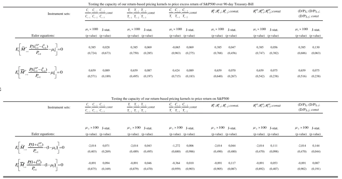
Table III presents single-equation equity-premium test results when return-based

pricing kernel estimates are used in place of consumption-based kernels. A variety of

macroeconomic and …nancial instruments, including up to their own two lags, are

em-ployed in testing. At the 5% signi…cance level, when gM_t is used, there is only one instance when theT J statistic rejects the null. This happens when the dividend-price

ratio Dt

Pt (up to its own two lags) is used as an instrument. When the mimicking portfolio is estimated using M_t, there is no rejection of the T J statistic at the 5%signi…cance level. Also, in all instances, estimates of ₁and ₂ obey ₁ = 0and ₂ = 0at the usual con…dence levels.

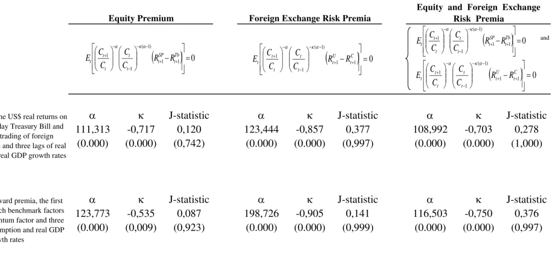
Table IV presents the …rst set of results regarding the forward-premium puzzle, in a

Table V presents tests, where gM_t and M_t are used to price the return on uncovered trading with foreign government bonds. In both tables, at the5%signi…cance level, there is not one single rejection either in mean tests for ₁and ₂ or for theT J statistic.

Table VI presents equity-premium tests for systems, whengM_t and M_t are used. No theoretical restriction is rejected here either by individual tests for ₁and ₂ or for the

T J statistic. Table VII presents system tests for the Fama-French portfolios. We do

not reject the null for the market excess return(Rm Rf)and for the small/big(SM B)

portfolio, but not for the high/low (HM L) one. It is worth stressing that, even then, the over-identifying-restriction test does not reject the null.

Finally, Table VIII presents system tests for the FPP when gM_t and M_t are used respectively. At 5% signi…cance, there is a single rejection (out of 10) of the over-identifying-restriction test for German bonds withM_t. Also, for British bonds, there is evidence that ₁ 6= 0, although the T J statistic does not reject the null.

4.4. Discussion

In this paper, we …rst questioned the standard testing procedure of the FPP, relying

on estimates _c0 and c1, obtained from running

st+1 st= 0+ 1(tft+1 st) +ut+1,

from a theoretical point of view. Our key point is that tft+1 st and ut+1 are

corre-lated, and that lagged observables are not valid instruments. Since these are exactly the

instrumental variables used in obtaining c0 and c1 , tests of the FPP relying on such

estimates are biased and inconsistent.

Next, we show evidence of the EPP in our data, if one takes the EPP to mean “the

failure of consumption-based kernels to explain the excess return of equity over

risk-free short term bonds with reasonable parameters values for risk aversion.” This is a

consequence of the results obtained in Table II, where system tests involving the returns

of these two assets overwhelmingly rejected the implied over-identifying restrictions, and

single-equation estimates of the risk-aversion coe¢cient were in excess of160, regardless of the preference speci…cation employed. A risk-aversion coe¢cient greater than 160 cannot be called “reasonable” under any circumstance, especially if it is obtained only

Recent work by Lustig and Verdelhan (2006a) estimates the coe¢cient of relative risk

aversion to …t an euler equation under more general preferences than those used in Mark

(1985) and Hodrick (1987) capable of pricing the returns on eight di¤erent portfolios

of foreign currencies. Because they do not try to price returns on these portfolios, one

cannot fully assess the adequacy of the pricing kernels they generate.

Next, we showed that, using return-based pricing kernels, in an euler-equation setup,

we are able to properly price returns and excess returns of assets that comprise the

equity premium and the forward premium puzzles; see results presented in Tables 3

through 8, where several econometric tests were performed, either in single equations or

in systems, and using two distinct estimates ofM_t –M_t andgM_t. These test results are very informative for at least two reasons. First, even if we do not have a consumption

model that delivers a proper pricing kernel, the mimicking portfolio is a valid kernel.

Second, our tests have an out-of-sample character in the cross-sectional dimension.

One important element of our testing procedure is that, when the ratio tFt+1=St

is used as an instrument, the theoretical restrictions tested were not rejected, leading

to the conclusion that tFt+1=St has no predictive power for Mt+1

Pt(1+it+1)

Pt+1

tFt+1 St+1

St . Hence, although the excess returns on uncovered over covered trading with foreign bonds

are predictable, “risk adjusted” excess returns are not. This raises the question that

predictability results using (1) may just be an artifact of the log-linear approximation of

the euler equation for excess returns. This is a very important result, since predictability

of st+1 st in (1) is a de…ning feature of the forward-premium puzzle.

Given that Mark (1985) found evidence of the FPP in proper econometric tests, also

found by Hansen and Singleton (1982, 1984) regarding the EPP23, and that we show

enough evidence that proper estimates of M_t do not misprice returns comprising the equity premium and the forward premium, we conclude that the EPP and the FPP

are “two symptoms of the same illness” – the poor (although steadily improving)

per-formance of current consumption-based pricing kernels to price asset returns or excess

returns. Our result takes the correlation with the pricing kernel as the appropriate

mea-sure of risk, and adds to the body of evidence that “explains” the forward premium as

a risk premium. The reason why we quote the term explains is because, we have not

tried to advance on the explanation of either puzzle, but simply to show that the two