Aspects of classical and quantum motion on a flux cone
E. S. Moreira, Jr.*Instituto de Fı´sica Teo´rica, Universidade Estadual Paulista, Rua Pamplona 145, 01405-900-Sa˜o Paulo, Sa˜o Paulo, Brazil ~Received 7 January 1998!
Motion of a nonrelativistic particle on a cone with a magnetic flux running through the cone axis~a ‘‘flux cone’’!is studied. It is expressed as the motion of a particle moving on the Euclidean plane under the action of a velocity-dependent force. The probability fluid~‘‘quantum flow’’!associated with a particular stationary state is studied close to the singularity, demonstrating nontrivial Aharonov-Bohm effects. For example, it is shown that, near the singularity, quantum flow departs from classical flow. In the context of the hydrodynami-cal approach to quantum mechanics, quantum potential due to the conihydrodynami-cal singularity is determined, and the way it affects quantum flow is analyzed. It is shown that the winding number of classical orbits plays a role in the description of the quantum flow. The connectivity of the configuration space is also discussed.
@S1050-2947~98!03508-2#
PACS number~s!: 03.65.Bz, 04.62.1v
I. INTRODUCTION
Usually, when the quantum description of a system is nontrivial, so is the classical one. However, this is not always the case. There is a number of examples whose intrinsic quantum effects do not have a classical analog. Notable among these is the Aharonov-Bohm ~AB! effect@1#. In this setup, the magnetic field vanishes everywhere except inside a thin flux tube. As there is no Lorentz force, classically par-ticles are free, and are not affected by the background. How-ever, in the quantum scattering problem the background leads to a nontrivial scattering, which is confirmed by experi-ment@2#.
The AB effect is a consequence of the interaction of quan-tum matter with a nearly trivial affine connection, and it is present in every gauge theory, including gravity. The analog of the AB setup in gravitation is a conical background@3–5#. The geometry is flat everywhere apart from a symmetry axis. As in the case of a thin flux tube, the problem of studying quantum mechanics on cones amounts to solving the usual equations in flat space with nontrivial boundary conditions. Solutions of these equations lead to geometrical Aharonov-Bohm effects @6–9#.
Quantum theory in conical backgrounds has been studied over two decades @10#, and investigations intensified in the mid 1980s@11#very much due to the importance in cosmol-ogy of cosmic strings. More recently, interest in the subject was renewed in the context of quantum mechanics of black holes, where one encounters conical singularities ~see, e.g., Ref. @12#, and references therein!. Besides these and other practical motivations to study quantum theory in conical backgrounds, there is another more academic one @6–9#. That is, the study of quantum mechanics in a nearly trivial gravitational background may shed some light on the pro-found problems of combining quantum mechanics and gen-eral relativity.
In this work classical and quantum effects caused by a conical singularity on the motion of a particle are studied. On
various occasions the AB setup is coupled to a conical ge-ometry~flux cone!, so that a comparison of the correspond-ing AB effects is possible. The paper is organized as follows. An account on the conical geometry and classical motion on a cone is given in Sec. II~this section comprises a review of early works by Deser, Gerbert, Jackiw, and ’t Hooft@13,6– 8#!, commenting on points which have been overlooked in the literature. In Sec. III, classical motion on a flux cone is studied. Quantization is implemented in Sec. IV, where the issue of boundary conditions at the singularity is considered, and a particular one is chosen, motivated by regularization arguments @14,15#. Corresponding stationary states are ob-tained and used to build up a state to probe the singularity. This leads, in Sec. V, to a study of quantum flow, showing nontrivial effects due to the conical singularity. Such effects are caused by a nonvanishing quantum potential whose fea-tures are mentioned. Connectivity of the configuration space is discussed by taking into account the behavior of quantum flow at the singularity. Sec. VI is a summary, including pos-sible extensions of this study. An account on the hydrody-namical approach to quantum mechanics ~whose elements are used in Sec. V!is given in the Appendix.
II. CONE
As mentioned previously this section is essentially a re-view of material in Refs. @13,6–8#. A cone is a two-dimensional space with a d-function curvature singularity
@16#. The line element may be written as
dl25gi jdxidxj
5
F
di j1~a2221!xixj
r2
G
dxidxj, ~1!
where the coordinate xi (i51,2) runs from 2` to` , r2 :5di jxixj anda is a positive parameter@13#. Imagining the
conical surface embedded in a three-dimensional Euclidean space, $x1,x2% are Cartesian coordinates on a plane perpen-dicular to the symmetry axis of the cone ~Fig. 1!. From Eq. *Electronic address: [email protected]
PRA 58
~1!, one sees that the conical singularity is located at the origin, and that, whena51, the cone becomes the Euclidean plane.
Using polar coordinates (x15rcosu, x2
5rsinu), Eq.~1!
can be rewritten as dl25a22dr2
1r2du2, where the conical
singularity is now hidden by the coordinate singularity at the origin. Note that the coordinates (r,u) and (r,u12p) label the same point, (r,u);(r,u12p). A further simplification of the line element can be made by rescaling$r,u% as
r5a21r, w5au, ~2!
resulting in dl25dr2
1r2dw2, showing the flatness of the
cone. However, as a consequence of the rescaling,
~r,w!;~r,w12pa!. ~3!
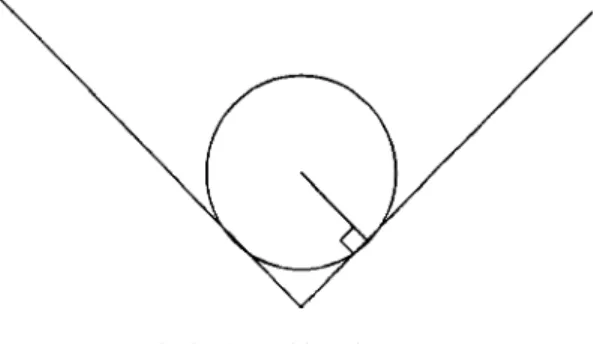
Coordinates$r,w% are polar coodinates on the surface of the cone. The angle of the missing wedge ~extra wedge, when a.1) is the deficit angle of the cone D52p(12a) ~Fig. 2!.
At this point it should be noted that the Euclidean plane and a cone have the same topology, differing in their geometry—the former is globally flat whereas the latter is not. To see this, one smooths the cone by replacing its tip by a tangential spherical cap of radius a ~Fig. 3!. Clearly the resulting surface is simply connected, a fact that does not change when a→0 and the idealized cone is recovered. Though the cone is a simply connected background, the
con-figuration space of a quantum particle living on it may be nonsimply connected~see Sec. V!.
It follows from Eq.~3!that the ‘‘Cartesian’’ coordinates defined by X1:5r coswand X2:5r sinw~Fig. 2!are singu-lar ifD5”0: in terms of$X1,X2% the metric tensor is Euclid-ean everywhere except on the rays defining the borders of the wedge, where these coordinates are discontinuous functions of w. ~Clearly the borders of the wedge can be arbitrarily rotated by redefining the interval of length 2pa over which w ranges.!Accordingly, the Levi-Civita connection vanishes everywhere except on the borders of the wedge, where it is singular. The nonvanishing connection ‘‘tells’’ the rest of the space that there is a curvature singularity at the origin, and this nontrivial behavior is the very one responsible for the geometrical Aharonov-Bohm-like effects that will be seen in this work.
Classical motion of a free particle with mass M on a conical surface may be determined from the Lagrangian,
L51
2M~dl/dt!
2
5a22
F
12M x˙
2
2~12a2 !
l
2
2 M r2
G
. ~4! The line element dl is given by Eq. ~1!, the dot denotes differentiation with respect to the time t, x:5(x1,x2), andl
:5x3M x˙ is the kinematical angular momentum~note thata3b:5ei jaibj). The Euler-Lagrange equations of motion,
i.e., the geodesic equations on the cone, follow from Eq.~4!,
M x¨52~12a2!
l
2M r3er, ~5!
where er:5x/r. One can regard Eq. ~5! as the equation of
motion of a particle moving on the Euclidean plane under the action of an angular-momentum-dependent central force, which is attractive for a,1 and repulsive for a.1 @17#. Clearly when
l
50 the motion is radial and uniform.The geometrical force in Eq. ~5! ranks somewhere be-tween an inertial force and a Newtonian force@5,18#. Indeed by changing from $x1,x2% to$X1,X2%, the force is ‘‘gauged away’’ everywhere apart from the borders of the wedge. Therefore, unless a51, trajectories crossing these rays are broken straight lines, with uniform motion ~dashed line in Fig. 2!. Integration of Eq. ~5! @7,18# shows that particles wind
w5@1/2a# ~6!
FIG. 1. Cone embedded in a three-dimensional Euclidean space.
FIG. 2. Singular Cartesian frame.
(@x#denotes the integral part of x) times around the conical singularity~Fig. 4!.
III. FLUX CONE
A cone may be immersed in a magnetic field pointing along its axis, and being homogeneous in that direction, by choosing a vector potential A(x,t) with a vanishing compo-nent in that direction. The Lagrangian of a particle with charge e moving in this background is given by
L
8
5L1ecx˙•A. ~7!
Thus the canonical momentum associated with x is
p5a22
F
M x˙1~a2
21!
l
r eu
G
1 ecA
5M x˙1~a22
21!M r˙er1
e
cA. ~8!
It follows from Eq. ~8!that
x3p5
l
1ecx3A, ~9!which is the usual expression for the canonical angular mo-mentum on the Euclidean plane. The Hamiltonian is given by
H5p•x˙2L
8
5a
2
2 M
S
p2 ecA
D
2
1~12a
2!
2 M r2
F
x3S
p2 ecA
DG
2
. ~10!
A magnetic flux F(t) running through the axis of the cone can be introduced by choosing
A5 F
2preu, ~11!
where eu:5(2sinu,cosu). Now there is a new singularity at the origin which is a d function magnetic field. Due to the cylindrical symmetry, the canonical angular momentum as given by Eq.~9!is conserved,
d
dt
S
l
1 eF2pc
D
50. ~12!The equations of motion following from Eq.~7!are given by Eq. ~5!, with the induced electric force 2e(]tF)eu/2pcr added on the right-hand side. This electric force prevents the orbital angular momentum
l
being a constant of motion, which is consistent with Eq.~12!. Clearly the above expres-sions reduce to the familiar ones on the plane @19#when a 51.The Aharonov-Bohm setup may be combined with the conical geometry by taking F constant, in which case the electric force vanishes, and Eq.~5!still holds. Obviously the same conclusion may be reached by realizing that the elec-tromagnetic Lagrangian in Eq. ~7! is a total derivative, eFu˙ /2pc, and consequently does not affect classical motion. However, as is well known @1#, this is not the case in quan-tum theory, which is the subject of the following sections.
@In the following sections, A is given by Eq. ~11!with con-stant F.#
IV. HAMILTONIAN OPERATOR AND STATIONARY STATES
The Hamiltonian operator H can be obtained from Eq.
~10!by the usual substitution@7#, p→2i\“. The invariance of the Schro¨dinger equation under the gauge transformation
A(x)→A(x)1“x(x), c(x,t)→exp$i(e/\c)x(x)%c(x,t) al-lows the choice x(x)5(2F/2p)u(x), thereby gauging away the vector potential everywhere, except on an arbitrary ray where the polar angle u is a discontinuous function of x
@20#. This singular gauge is analogous to the singular Carte-sian coordinates$X1,X2%. It might have been anticipated that
A cannot vanish everywhere around the origin since
rA•dx5F. Similar reasoning may be applied to the Levi-Civita connection of a conical geometry ~see Ref.@21# and references therein!.
Definings:52eF/ch, the transformed wave function is
c
8
~x,t!5exp$isu%c~x,t!. ~13!It then follows from Eq. ~10!,~2!, and~3!that
H52 \
2
2 M 1 r
] ]r
S
r] ]r
D
1L2
2 Mr2, ~14!
c~r,w12pa!5exp$i2ps%c~r,w!, ~15!
where
L:52i\ ]
]w ~16!
and the prime in c
8
has been dropped. As H in Eq.~14! is just the free Hamiltonian operator on the plane written in polar coordinates@which is not surprising since$X1,X2% is a~singular!Cartesian frame#, the interaction with the magnetic flux and the conical geometry manifest themselves only through Eq.~15!. In fact the twisted boundary condition~15!
states that the wave function is not single valued for nonin-teger values of the flux parameter s, and therefore is not
continuous along some ray. This corresponds to~and is com-patible with!the fact that H, as given by Eq.~14!, disguises a singular vector potential which, as mentioned above, is not defined everywhere. Note also that, according to Eq.~15!,c must either vanish or diverge at the origin ~for noninteger s), otherwise an inconsistency results when a loop is shrunk aroundr50 @22#.
Considering Eqs.~14!and~15!, it follows from the Schro¨-dinger equation
d
dt
E
0` dr r
E
0 2pa
dw cc*5lim r→0
E
02pa
dw rJr, ~17!
whereJr is the usual expression for the radial component of the probability current on the plane,
Jr51
MRe
F
c*\
i ]c
]r
G
, Jw5 1 MReF
c*\
ir ]c
]wG. ~18!
In obtaining Eq. ~17!, it has been assumed that the wave function vanishes at infinity. The right-hand side of Eq.~17!
is the net probability crossing an infinitesimally small circle around the singularity. Equating Eq.~17!to zero amounts to the statement that the singularity at the origin is neither a source nor a sink ~probability is conserved!, which is auto-matically guaranteed if
lim r→0
E
02pa
dw r
S
c*]f ]r2]c*
]r f
D
50. ~19!Expression ~19! is the condition for self-adjointness of the Hamiltonian operator~14!,
^
cuHuf&
5^
fuHuc&
*.If Rk,m(r) are functions such that
F
r ] ]rS
r] ]r
D
2S
m1s a
D
2
1~kr!2
G
Rk,m~r!50, ~20!
then
ck,m~r,w!5
1
A
2paRk,m~r!ei~m1s !w/a, ~21!
where 0<k,` and m is an integer, are simultaneous eigen-functions of H and L with eigenvalues \2k2/2M and (m
1s)\/a, respectively. Note that the effect of the magnetic flux and of the conical geometry on the eigenvalues of L is to shift and to rescale them, respectively. For a particle with spin there is also a shift due to a coupling between the spin and the deficit angle@8,23#.
In order that the stationary states ck,m span a space of
wave functions in which probability is conserved, they must satisfy Eq. ~19!,
lim r→0
r
S
Rk8,m
* ]Rk,m ]r 2
]Rk
8,m
*
]r Rk,m
D
50, ~22!where the orthonormality relation *02padwexp$iw(m 2n)/a% 52padmnhas been used. Expression~22!is the condition for
self-adjointness of the square of the operator Pr:52i\(]r 11/2r), and is itself self-adjoint if
lim r→0
r~fc*!50, ~23!
as may easily be shown by equating *0`drr@f( Prc)* 2c*( Prf)# to zero. One sees from Eq.~23! that Rk,m(r)
may diverge mildly at the origin@which also applies toJrin Eq.~17!#, and still be compatible with conservation of prob-ability. A mild divergence would not spoil the square inte-grability of the wave function, since a behaviorc;1/rnwith n,1 yields *0edr rucu2}e2(12n), which vanishes with e.
Note that in order to satisfy Eq. ~23!one must have n,12.
Obviously a logarithmic divergence also passes this test, since it is weaker than the 1/rn divergence.
In the following only wave functions which are finite at the singularity will be considered. In quantum mechanics on the flux cone, finiteness is motivated by the fact that it arises naturally when the singularities are smoothed by some regu-larization procedure@14,15#.~Divergent wave functions were considered in Refs. @14,15#.! Therefore, one takes as solu-tions of Eq.~20!Bessel functions of the first kind,
Rk,m~r!5Jum1su/a~kr!, ~24!
which being finite at the origin satisfy Eq. ~23! and conse-quently Eq. ~22!. As a check we may verify that Eq. ~24!
indeed satisfies Eq.~22!by observing that
dJn~x!
dx 5 1
2@Jn21~x!2Jn11~x!#. ~25!
Hence the complete set of stationary states ck,m is given by
Eqs. ~21!and~24!.
A particular state to probe the singularity can be found as follows. The general expression for a stationary state of en-ergy\2k2/2M is given by
ck~r,w!5
(
m52``
cmck,m~r,w!. ~26!
The coefficients cm are determined by considering the
Fou-rier expansion of a plane wave
exp$2ia cosf%5
(
m52` `
~2i!umuJ
umu~a!eimf, ~27!
and letting the magnetic flux and the conical geometry act on it. This involves shifting and rescaling the angular momen-tum of the modes, as mentioned previously, leading to
cm~d,a !:5
A
2paexpH
2ip2aum2du
J
, ~28!where the flux parameter has been redefined to be d:52s in order to compare the result with earlier work. The station-ary state ~26! with cm5cm
(d,a) will be denoted c
k
(d,a).
Clearly,
ck
~0,1!~r,w!
5exp$2ikrcosw%
~Note that whena51, both$x1,x2%and$X1,X2%are genuine Cartesian coordinates which coincide.! The stationary states c(d,1) andc(0,a) have previously been considered in the
lit-erature~in Refs.@1#and@9,7#, respectively!in the context of scattering. Section V considers the probability fluid~see the Appendix!associated withck
(d,a).
V. QUANTUM FLOW
Consider the symmetries of the stateck
(d,a). By redefining
the summation index in Eq. ~26!, it is straightforward to show that
ck
~d1n,a !~r,w! 5ck
~d,a !~r,w!, ~30! from which it follows that integer flux parameters are equivalent to zero. Also,
ck
~2d,a !~r,w! 5ck
~d,a !~r,
2w! ~31!
implies that for vanishing flux parameter ck(0,a)(r,u) [ck(0,a)
(r,2u). Thus the quantum flow is symmetric with respect to the x1axis and, consequently, no probability from the upper half-plane passes to the lower half-plane, and vice versa. In other words the current lines associated with the quantum flow must not cross the x1 axis; otherwise, due to the symmetry, they would intercept on this axis. When the flux parameter is switched on this symmetry is broken, im-plying that the flow corresponding to a charged particle is sensitive to the direction~up or down!in which the magnetic flux runs. By studying symmetries ~30! and ~31!, one sees that
0<d<1
2 ~32!
covers all possible behaviors of the flow, and thatd51 2 also
yields a flow symmetric with respect to the x1 axis.
Expres-sions~30!and~31!generalize the known symmetries@24,2#
of the AB setup to include the presence of a conical singu-larity.
Considering Eqs. ~26!and~28!, the probability density
ck ~d,a !c
k ~d,a !*
5
(
m,m852` `
exp$iQm,m
8
~d,a !
~w!%
3Jum2du/a~kr!Jum82du/a~kr! ~33! follows, where
Qm,m
8
~d,a !
~w!:5aF1 ~um2du2um
8
2du!p22~m2m
8
!wG
,~34!
satisfying Qm,m
8
(d,a)
52Qm
8,m (d,a)
. The probability current, when expressed with respect to $X1,X2%, has the familiar polar
components on the Euclidean plane ~18!, from which it fol-lows that
Jr~d,a !~r,w!52 M\k
(
m,m852` `
sin$Qm,m
8
~d,a !
~w!%Jum2du/a~kr!
3@Jum82du/a21~kr!2Jum82du/a11~kr!# ~35!
and
Jw~d,a !~r,w!5 \
Mrm,m
(
852` `m
8
2da cos$Qm,m8 ~d,a !
~w!%
3Jum2du/a~kr!Jum82du/a~kr!. ~36! In deriving Eq.~35!, equality~25!has been used.
In the following the quantum flow will be studied when
kr!1. ~37!
This amounts to considering the expansion
Jn~z!5
S
2zD
nF
1G~11n!2
1
G~21n!
S
z
2
D
2
1O~z4!
G
~38!in Eqs. ~33!, ~35!, and ~36!, keeping only the terms with small m and m
8
. For simplicity the cone and the flux tube will be considered separately. It should be remarked that Eq.~37! contrasts with the regime on scattering problems for which kr@1.
A. Conical singularity
Using Eqs.~34!and~38!, it follows from Eq.~33!that the first terms of the probability density around a conical singu-larity are
ck~0,a !c k ~0,a !*
511cos$p/2a%cos$w/a% 21/a22G~111/a! ~kr!
1/a
212~kr!2
1 a
2
22/a21
F
11cos$2w/a%
G2~1/a!
1cos$p
/a%cos$2w/a% aG~2/a!
G
~kr!2/a, ~39!
where all terms of the order of (kr)l, withl<2 and 12,a
,32, have been considered. When a51 the corresponding
~nonzeroth! powers of kr in Eq. ~39! cancel out, as they should, since in the absence of the conical singularity~and of magnetic flux!the probing state becomes a plane wave@see Eq. ~29!#.
In studying the probability density~39!, one may be led to conclude that the configuration space of a particle in the state ck
(0,a) is simply connected, sincec
k
(0,a)c
k
(0,a)* does not
hole, and the current lines surround the disc without crossing it. This is a nonsimply connected configuration space. When the disc degenerates to a point at the origin, this picture does not change. At the origin, which is now the border of the disc, the radial probability current vanishes. It is reasonable to say that the configuration space of this particle is R2 2$0%, although the probability density may be nonvanishing at the origin. If this interpretation is adopted, it follows that before making any statement about the connectivity of the configuration space of a particle on the cone, one should also study the probability current at the singularity.
Before determining the behavior of the probability current at the conical singularity, consider its corresponding quan-tum potential~A2!. The term containing (kr)1/a in Eq. ~39!
satisfies the Laplace equation and, consequently, does not give any information about the quantum potential@that is the reason why higher order corrections in Eq.~39!were consid-ered#. For 1
2,a, 3
2, it follows from Eqs.~A2!and~39!that
the quantum potential near the conical singularity is approxi-mately given by
Va~r!52~ \k!
2
2 M
~kr/2!2/a22
G2
@1/a# , ~40!
where an unimportant constant has been dropped. The fact that Eq.~40!is not a constant when the conical singularity is present (aÞ1) constitutes a genuine quantum-mechanical effect~a geometrical Aharonov-Bohm effect!. Far away from the conical singularity, for positive X1, the state c(0,a,1/2)
behaves approximately as the plane wave~29! @9,7#. Conse-quently, in terms of $X1,X2%, the current lines of the quan-tum flow are approximately straight lines parallel to the X1 axis, running to the left. At this stage, the quantum flow coincides with a flow of classical particles ~see Sec. II!. As the singularity is approached, the two flows depart from each other. Near the conical singularity they differ radically—by differentiating the quantum potential~40!, it follows that the current lines are scattered away from the conical singularity whena,1 and bent toward it whena.1, whereas the clas-sical particles experience no force ~in the $X1,X2% frame!.
When a51, the quantum potential ~40! becomes constant and the classical and quantum flows coincide everywhere, as they must.
After this rather qualitative analysis, the probability cur-rent will now be determined near the conical singularity. By proceeding as one did to obtain Eq.~39!, from Eqs.~35!and
~36!it follows that
Jr~0,a !~r,w!52\Mk
S
k2rD
1/a21
F
sin$p/2a%cos$w/a%G~1/a!
1sin$p/a%cos$2w/a% 21/aG~2/a! ~kr!
1/a
G
~41!and
Jw~0,a !~r,w!5\k
M
S
kr2
D
1/a21
F
sin$p/2a%sin$w/a%G~1/a!
1sin$p/a%sin$2w/a% 21/aG~2/a! ~kr!
1/a
G
, ~42! where terms O@(kr)2# and O@(kr)2/a# have been omitted for a<1 ora.1, respectively. When 1/a is even, one sees that expressions ~41! and ~42! vanish, which is consistent with the fact that the stationary state ck(0,1/2n)is a real func-tion@7#. This effect becomes more intuitive by recalling that for even 1/a classical particles are scattered backwards, and then the scattered classical flow cancels the incident one, resulting in a vanishing net classical flow. Clearly when a51, Eqs. ~41! and ~42! imply that Jr(0,1)(r,w) 52(\k/ M )cosw andJw(0,1)(r,w)5(\k/ M )sinw, which are the polar components of the plane-wave probability current,
J~0,1!~r,w!52\k
M e1 ~43!
@e1:5(1,0)#, as expected. From Eqs.~41!and~42!, one sees
that in the limitr→0 the probability current either vanishes or diverges for a,1 and a.1, respectively. Note that al-thoughJr(0,a.1)diverges asr→0, the right-hand side of Eq.
~17!vanishes, which is not surprising since this was the cri-terion for choosing the stationary states. The fact that fora ,1 the quantum flow avoids the conical singularity suggests that the corresponding configuration space is nonsimply con-nected~and vice versa fora>1), as discussed previously. At this point it should be remarked that according to the authors of Ref. @15#, ifcÞ0 at the conical singularity, the configu-ration space is simply connected and, consequently, two identical particles on the plane (a512) in the state c
‘‘col-lide.’’ The analysis of the quantum flow above seems to suggest that this may be not the case.
Due to the presence of the wedge in the singular Cartesian coordinates $X1,X2%, for some purposes it is more conve-nient to describe the flow in terms of the embedded Cartesian coordinates $x1,x2%. By performing the coordinate transfor-mation Xi→xi it is straightforward to show that, in the
$x1,x2% frame, the probability current is given by j5
j
rer1
j
ueu, withj
r5aJr andj
u5Jw. ~Note that the wave function and j satisfy the usual Cartesian form of the conti-nuity equation.!Then, keeping only the leading contribution in Eqs.~41!and~42!, one findsj~0,a !~r,u!52\k
M
S
kr 2aD
1/a21sin$p/2a%
G~1/a!
3@e11~a21!cosuer#, ~44!
where the features mentioned above may easily be verified. For example setting a51 in Eq.~44!reproduces Eq.~43!.
Figures 5, 6, and 7 show the current lines associated with
j(0,a) for a,1, a51, anda.1. They have been obtained by plotting the numerical integration of the equations result-ing by equatresult-ing dx/dl to the term between brackets in Eq.
dx1
dl 511~a21!
~x1!2
~x1!2
1~x2!2,
dx2
dl 5~a21!
x1x2
~x1!2
1~x2!2,
wherel is an arbitrary parameter.
At u50, 6p/2, andp, the flow runs parallel to the x1
axis, as may be seen from Eq.~44!. As the direction of j(0,a) in Eq.~44!for a givena is determined byu only, the current lines are parallel to each other ~a feature shared with the classical flow!. However, this is true only very close to the singularity, where the subleading contributions in Eqs. ~41!
and~42!are not relevant. Apart from diverging at the conical singularity fora.1, the probability current is smooth every-where.
Consider more carefully the factor f (r,D):5(kr)1/a21 in Eq. ~44!. For an infinitesimal e.0, f (0,01e)50, f (0,0) 51, and f (0,02e)5`. This discontinuity makes the behav-ior of the quantum flow on the Euclidean plane change abruptly in the presence of a tiny deficit angle. No such effect exists at the classical level, where the velocity of the particles varies smoothly with the deficit angle. This effect is less surprising when recalling that even a tiny deficit anglee corresponds to a d-function curvature which ‘‘pierces’’ the configuration space.
An unsuspected relationship between the winding number of classical orbits and the quantum flow arises when studying the direction of the latter @left or right, with the flow ~43!
running to the left#. Such direction is determined by the fac-tor sin$p/2a% in Eq. ~44!. For a.1
2, the quantum flow
al-ways runs to the left, and the classical particles are scattered without winding around the conical singularity. For a512
~classical backward scattering! the quantum flow stops and reverses its direction for a,12, with the classical particles
winding once around the conical singularity. It continues to run to the right until one decreases a to 14 when another
classical backward scattering takes place with another inter-ruption of the flow. By further decreasing a, the quantum flow starts to run to the left, while the classical particles wind twice around the conical singularity. Generically, the direc-tion of the quantum flow is controlled by the winding num-ber w defined in Eq.~6!—the quantum flow runs to the left for even w and to the right for odd w.
From Fig. 5, one sees that for a,1 the quantum flow negotiates the conical singularity in a manner similar to the
one in which a low velocity fluid negotiates a cylinder. This analogy may be taken as an evidence that the configuration space is not simply connected whena,1, as was suggested above. Note that there are no vortices present anywhere since the magnetic flux is switched off@observe Eq.~A5!#.
B. Flux tube
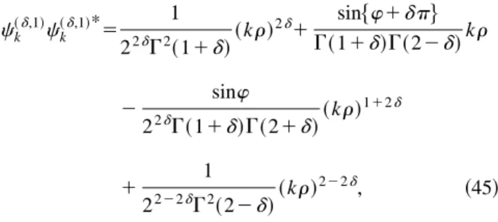
Now consider nonvanishing magnetic flux in the absence of a conical singularity. The analog of Eq.~39!is
ck~d,1!c k ~d,1!*
5 1
22dG2
~11d!~kr! 2d
1G~1sin$w1dp% 1d!G~22d!kr
2 sinw
22dG~11d!G~21d!~kr! 112d
1 1
2222dG2
~22d!~kr!
222d, ~45!
where all terms of order (kr)lwere taken into account, with
l<1, and Eq. ~32!was considered. Expression ~45!agrees with the one in Ref. @2#, where a slightly different method was used. Ford50, Eq.~45!reduces to unity up to a (kr)2
term, which would be canceled if higher powers of kr in Eq.
~45! had been kept. For a nonvanishing flux parameter, the probability density vanishes at the flux tube (r50) and the corresponding configuration space is nonsimply connected. The expression for the quantum potential corresponding to Eq. ~45!will not be given here. Instead a study of the prob-ability current itself is carried out in the following.
As in the case of the conical singularity, Eqs. ~35! and
~36! may be used to obtainJr(r,w) andJw(r,w). Expres-sions which correspond to Eqs. ~41! and ~42! were previ-ously found in Ref. @2# ~see also Ref.@24#!. Study will be limited to the case where the flux parameter is very small, viz.d!1. In so doing, J5Jrer1Jwew reads approximately
FIG. 5. Quantum flow whena,1.
FIG. 6. Quantum flow whena51.
J~d,1!~r,w!5\Mk
F
ed2d
krew
G
, ~46!where ed is the unit vector er evaluated at w5p(12d/2). When d50, Eq. ~46! reduces to Eq. ~43!, as should be. Clearly J vanishes when ew5ed and kr5d, so that
~r,w!5@d/k,p~12d!/2#. ~47!
It is also clear from Eq. ~46! that the quantum flow~under the action of the corresponding quantum potential!circulates around the origin when it is close to the origin@24#. It turns out that Eq. ~47! is a stagnation point, and that there is a vortex around the flux tube, which was expected by observ-ing Eq. ~A5!. In Fig. 8, the numerical solution of
dx1
dl 5211~d/k!
x2
~x1!21~x2!2,
dx2
dl 52~d/k!
x1
~x1!2
1~x2!2
is plotted, showing the main features of the quantum flow near the flux tube. This is in agreement with Ref.@2#, where the analytical expression for the current lines was given.
One sees from Eq.~46!that, as with the conical singular-ity, the d function magnetic field at the origin imparts a discontinuous change in the quantum flow of a charged par-ticle. Any tiny amount of magnetic flux changes the topology of the current lines ~open lines become loops! near the ori-gin. From Fig. 8 one sees that, as previously mentioned, the presence of the magnetic flux breaks the symmetry with re-spect to the X1 axis. Notice that, as the distance from the
origin increases ~still for kr!1), the flow gradually aproaches that of a plane wave @Eq. ~43!#, unlike the effect caused by the conical singularity. An important distinction between the effects caused by the conical singularity and the magnetic flux is that the latter only affects charged particles
(dÞ0), whereas the former affects all particles indifferently. This fact may be seen as a manifestation of the equivalence principle—geometrical Aharonov-Bohm effects due to a conical singularity do not depend on any particle attribute.
VI. SUMMARY
Summarizing, it was shown that the motion of a particle on a flux cone can be regarded as a motion under the action of an angular-momentum-dependent central force. Due to lo-cal flatness, quantization was implemented along usual pro-cedures in flat space. By studying the probability fluid cor-responding to a particular stationary state~‘‘plane wave’’ on a flux cone!, interesting effects were found. For example, it was shown that the winding number of classical orbits con-trols the direction of the quantum flow on a cone. Classical flow~which is nearly trivial!and quantum flow were shown to depart from each other near the singularity due to the presence of a nonvanishing quantum force. For the case of a conical singularity, the corresponding quantum potential was determined and analyzed. The issue of connectivity of the configuration space was treated and some interpretations were proposed.
Other boundary conditions at the singularity ~those con-sidered in Refs.@14,15#!may lead to interesting effects. An-other interesting extension of this work would be to consider relativistic particles. The use of this approach in the study of quantum flow in the context of other geometries and topolo-gies would be worthwhile, particularly in geometries with horizons.
ACKNOWLEDGMENTS
The author is grateful to George Matsas for reviewing the manuscript and for clarifying discussions. The work was supported by FAPESP Grant No. 96/12259-1.
APPENDIX: HYDRODYNAMICAL APPROACH TO QUANTUM MECHANICS
Analogies between quantum mechanics and fluid dynam-ics do not stop at a continuity equation which expresses local conservation of probability. The Schro¨dinger equation can be rephrased as a set of hydrodynamical equations~see Ref.@2#, and references therein!. In order to derive them, consider a particle with charge e moving in the Euclidean space ~the generalization to arbitrary backgrounds is straightforward!
under the action of an electromagnetic field (E,B) with cor-responding potentials (f,A). The Hamiltonian operator is then given by
H5 1
2 M
S
2i\“2 e cAD
2
1ef.
Now one rewrites the solution c for the corresponding Schro¨dinger equation as
c~t,r!5̺~t,r!eix~t,r!.
The real part of the Schro¨dinger equation reads
\]x
]t1
\2
2 M
F
“x2 ec\A
G
21ef1V50, ~A1!
where
V~t,r!:52 \
2
2 M
¹2 ̺
̺
[2 \
2
2 M
¹2~cc*!1/2
~cc*!1/2 . ~A2!
The imaginary part reads
]̺2
]t 1“ •~̺
2v!
50, ~A3!
with v:5@\“x2eA/c#/ M , leading to the constraint
“3v52 e
M cB. ~A4!
Now one sees that̺2v is the probability current, and
there-fore Eq. ~A3! is just the continuity equation. Note that by integrating Eq. ~A4!along a closed loop, it follows that
R
v•dl52eFM c, ~A5!
whereF is the magnetic flux enclosed by the loop.
The last step is to apply“in Eq.~A1!, after which one is left with a set of equations of motion for a fluid of density̺2
and velocity v,
M d
dtv~t,r![M
F
]v]t1~v• “!v
G
5eE1ecv3B2“V. ~A6!
Thus the wavelike Schro¨dinger equation@where the function to be determined isc for a given configuration of potentials (f,A)#has been replaced by the hydrodynamical equations
~A3!and~A6!with the constraint~A4! @where the functions to be determined are (̺,v) for a given configuration of elec-tromagnetic field (E,B)#. These equations govern the behav-ior of the quantum flow.
Whereas the Schro¨dinger equation is more appropriate to study wavelike features of quantum mechanics, the hydrody-namical equations are more appropriate to study particlelike features. To see this, assume that the quantum force2“V in Eq.~A6!is negligible when compared with the Lorentz force
~and other forces that one might have considered!. In this ‘‘classical limit,’’ Eq.~A6!reduces to the equations of mo-tion for a flow of noninteracting classical particles. Note that Eq. ~A1! is the corresponding Hamilton-Jacobi equation, where the action is identified with \x. It is clear that the quantum potential V represents the departure from the clas-sical motion. In regions where the quantum potential is rel-evant, the classical and quantum flows may differ consider-ably from each other. For example, in a region of vanishing field strengths the motion of the classical flow is trivial, since the Lorentz force vanishes there. The motion of the quantum flow, on the other hand, may be quite elaborate due to the presence of the quantum force2“V in Eq.~A6!. A nonva-nishing quantum force is the essence of Aharonov-Bohm-like effects.
@1#Y. Aharanov and D. Bohm, Phys. Rev. 115, 485~1959!.
@2#S. Olariu and I. I. Popescu, Rev. Mod. Phys. 57, 339~1985!.
@3#L. Marder, Proc. R. Soc. London, Ser. A 252, 45~1959!.
@4#A. Staruszkiewicz, Acta Phys. Pol. 24, 734~1963!.
@5#J. S. Dowker, Nuovo Cimento B 52, 129~1967!.
@6#G. ’t Hooft, Commun. Math. Phys. 117, 685~1988!.
@7#S. Deser and R. Jackiw, Commun. Math. Phys. 118, 495
~1988!.
@8#P. S. Gerbert and R. Jackiw, Commun. Math. Phys. 124, 229
~1989!; P. S. Gerbert, Nucl. Phys. B 346, 440~1990!.
@9#D. Lancaster, Ph.D. thesis, Stanford University,~1984!; Phys. Rev. D 42, 2678~1990!.
@10#J. S. Dowker, J. Phys. A 10, 115 ~1977!; Phys. Rev. D 18, 1856~1978!.
@11#A. G. Smith, in The Formation and Evolution of Cosmic
Strings, edited by G. W. Gibbons, S. W. Hawking, and T.
Vachaspati ~Cambridge University Press, Cambridge, 1990!; T. M. Helliwell and D. A. Konkowski, Phys. Rev. D 34, 1918
~1986!; B. Linet, ibid. 35, 536~1987!; V. P. Frolov and E. M. Serebriany, ibid. 35, 3779~1987!; J. S. Dowker, ibid. 36, 3095
~1987!; 36, 3742~1987!.
@12#S. Zerbini, G. Cognola, and L. Vanzo, Phys. Rev. D 54, 2699
~1996!.
@13#S. Deser, R. Jackiw, and G. ’t Hooft, Ann. Phys.~N.Y.!152,
220~1984!.
@14#B. S. Kay and U. M. Studer, Commun. Math. Phys. 139, 103
~1991!.
@15#M. Bourdeau and R. D. Sorkin, Phys. Rev. D 45, 687~1992!.
@16#D. D. Sokolov and A. A. Starobinskii, Dok. Akad. Nauk 234, 1043~1977! @Sov. Phys. Dokl. 22, 312~1977!#.
@17#E. S. Moreira, Jr., Ph.D. thesis, University of London, 1997.
@18#G. Cle´ment, Int. J. Theor. Phys. 24, 267~1985!.
@19#R. Jackiw and A. N. Redlich, Phys. Rev. Lett. 50, 555
~1983!.
@20#B. Felsager, Geometry, Particles and Fields~Odense Univer-sity Press, Odense, 1981!.
@21#V. B. Bezerra, J. Math. Phys. 30, 2895~1989!.
@22#P. A. M. Dirac, Proc. R. Soc. London, Ser. A 133, 60
~1931!.
@23#E. S. Moreira, Jr., Nucl. Phys. B 451, 365~1995!.