A R C H I V E S
o f
F O U N D R Y E N G I N E E R I N G
Published quarterly as the organ of the Foundry Commission of the Polish Academy of Sciences
ISSN (1897-3310)
Volume 8
Issue 4/2008
105 – 110
20/4
Identification of boundary heat flux
on the continuous casting surface
E. Majchrzak
a b*, B. Mochnacki
b, M. Dziewo
ń
ski
a, M. Jasi
ń
ski
aa
Department for Strength of Materials and Computational Mechanics
Silesian University of Technology, Konarskiego 18a, 44-100 Gliwice, Poland
b
Institute of Mathematics and Computer Science
Cz
ę
stochowa University of Technology, D
ą
browskiego 73, 42-200 Cz
ę
stochowa, Poland
*Corresponding author. E-mail address: [email protected]
Received 04.06.2008; accepted in revised form 09.07.2008
Abstract
In the paper the numerical solution of the inverse problem consisting in the identification of the heat flux on the continuous casting surface is presented. The additional information results from the measured surface or interior temperature histories. In particular the sequential function specification method using future time steps is applied. On the stage of numerical computations the 1st scheme of the boundary element method for parabolic equations is used. Because the problem is strongly non-linear the additional procedure 'linearizing' the task discussed is introduced. This procedure is called the artificial heat source method. In the final part of the paper the examples of computations are shown.
Keywords: Application of information technology to the foundry industry, Solidification process, Numerical techniques, Inverse problems, Boundary element method
1. Introduction
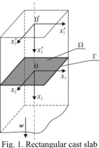
The vertical, rectangular cast slab is considered (Figure 1). Neglecting the convection proceeding in the molten metal sub-domain, the thermal processes in the continuous casting volume are described by the following equation [1]
( )
(
',)
(
)
( )
(
)
grad ', div grad ',
T x t
C T T x t T T x t
t
⎡∂ ⎤
+ ⋅ = ⎡λ ⎤
⎢ ∂ ⎥ ⎣
⎣ w ⎦ ⎦ (1)
where x'={ ',x1 x2',x3' }. The casting shifts in axis x
3′ direction
and its pulling rate is equal to w (more precisely, the velocity field
in domain considered: ). The same mathematical
description can be used in a case of so-called radial plants,
because a large radius of plant curvature (in comparison to the casting dimensions) allows to treat the radial installation as a vertical one.
[0, 0, ]w
=
w
On the upper surface of the casting (free surface of molten metal) the boundary condition of the 1st type (pouring temperature) can be taken into account. On the conventionally assumed bottom surface limiting the domain considered (it is a
region of final cooling zone) we can put ∂ ∂ , this means the adiabatic condition. On the lateral surface the Neumann condition is assumed (the data concerning the boundary heat fluxes are collected in [2]).
/ 0
Fig. 1. Rectangular cast slab
The initial condition resolves itself into the assumption, that a certain layer of molten metal directly over the starter bar has a pouring temperature. The starter bar allows to shut the continuous casting mould during the plant starting.
The numerous experiments show that conductional component of heat transfer corresponding to the direction of casting displacement is very small (this component constitutes about 5% of the heat conducted from the axis to the lateral
surfaces), this means that the component div⎡λ⎣
( )
T gradT⎤⎦ can be simplified to the form( )
( )
( )
1 1 2
div grad
' ' '
T T
T T T T
2'
x x x x
⎡ ⎤ ⎡
∂ ∂ ∂ ∂
⎡λ ⎤ = ⎢λ ⎥+ ⎢λ
⎣ ⎦ ∂ ⎣ ∂ ⎦ ∂ ⎣ ∂ ⎤⎥
⎦ (2)
A pretty interesting and effective in numerical simulation variant of mathematical approach to the continuous casting problem was presented by the authors of this paper in [3, 4]. The algorithm has been called 'a wandering cross section method'.
Let we rewrite the equation (2) in coordinate system 'tied' to a
certain section Ω of shifting casting, namely
1 1' , 2 2' , 3 3' .
x =x x =x x =x −w t
We assume, as previously, that the heat conduction in x3′ direction can be neglected. It is easy to
check up that we 'lose' in energy equation the component grad
w⋅ T
(
1 2)
( )
( )
( )
1 1 2
, : T T
x x C T T T
t x x x x
⎡ ⎤ ⎡
∂ ∂ ∂ ∂ ∂
∈ Ω = ⎢λ ⎥+ ⎢λ ∂ ∂ ⎣ ∂ ⎦ ∂ ⎣ ∂ 2
T⎤
⎥
⎦ (3)
The last equation corresponds to typical thermal diffusion equation for a 2D object oriented in cartesian coordinate system (but finally we find the 3D solution). It should be solved for initial condition T(x1, x2, 0)=T0 (pouring temperature), while the
boundary heat flux on the perimeter Γ of the section considered is the function of time.
In the paper the 2D task concerning the continuous casting technology is discussed. On the basis of the knowledge of temperature history at the selected set of the points from the casting domain the boundary heat flux is identified [5, 6, 7]. The identification of the boundary heat flux in the primary cooling
zone (continuous casting mould) has been done using sequential function specification method [6, 7]. The results of computations are presented in the final part of the paper.
2. Identification of boundary heat flux
In this chapter the sequential function specification method using future temperature information is presented [6, 7]. This method allows to estimate the boundary heat flux on the basis of temperature measurements in the casting domain.
If we assume the constant value of thermal conductivity
( )
Tλ = λ
(this assumption in the case of typical alloys is acceptable) then the problem discussed is of the form (c.f. equation (3))
( ) ( )
( )
( )
( )
( )
2
0
,
: ,
,
: ,
0 : ,
T x t
x C T T x t
t
T x t
x q x t
n
t T x t T
⎧ ∈ Ω ∂ = λ∇
⎪ ∂
⎪⎪ ∂
⎨ ∈Γ = −λ
⎪ ∂
⎪
⎪ = =
⎩ (4)
where x={x1, x2} and
( )
2( )
2( )
2
2 2
1
, ,
, T x t T x t
T x t
x x
∂ ∂
∇ = +
∂ ∂ 2 (5)
We define the substitute thermal capacity C(T) for T∈[TS ,TL] in the form of polynomial
( )
2 30 1 2 3 4
C T =c +c T+c T +c T +c T4
(6)
which fulfills the conditions:
i. For T=TS : C(TS )=cS and for T=TL:C(TL)=cL, where cS, cL are the volumetric specific heats of solid and liquid states, respectively.
ii. For T=TS and T=TLdC(T)/dT=0.
iii. The change of enthalpy connected with the solidification equals
( )
d(
)
L
S
T
P L S
T
C T T= +L c T −T
∫
(7) where cp is the volumetric specific heat of mushy zone.
(
1, 2,)
, 1, 2, ..., , 1, 2, ...,f i i f
d i d
T =T x x t i= M f = F
(8)
where M is the number of sensors.
In sequential function specification method [6, 7] it is assumed that the heat flux is known at the set of boundary points
j , j
x ∈ Γ =1,2,..., J for times t 1
, t 2, ..., t f − 1, and we want to
determine the heat flux
(
1, 2,)
f j j f
j
q =q x x t
at time .tf Additionally, the temperature values are known for R future intervals, namely (r=1, 2, ..., R)
(
)
1 1
, , 1, 2, ...,
f r i f r
d i d
T + − =T x t + − i= M
−
(9)
and we assume that the heat flux is constant over R future steps and equal to the heat flux at time t f
1 1
...
f f f R
j j j
q =q + = =q +
(10)
In order to solve the inverse problem, the least squares method is applied [5, 6, 8]
(
1 1)
21 1
M R
f r f r
i d i
i r
S T + − T + −
= =
=
∑∑
−(11)
Function is expanded in a Taylor
series about arbitrary but known value of heat flux
(
)
1 1
,
f r i f r
i
T + − =T x T + −
*f j q
(
)
* 11 * 1 *
1 f f
j j
f r J
f r f r i f
i i f j
j j q q
T
T T q q
q + − + − + − = = ∂ = + − ∂
∑
f j (12) where 1 *f r iT + −
denotes the calculated temperature at point x i for
time
1
f r i
t + −
obtained under the assumption that for
the heat fluxes equal
1 1
[ f , f r ] t∈t − t + −
1 ... 1 *
f f f R f
j j j
q =q + = =q + − =qj
We introduce the sensitivity coefficients [3, 4] and then
(
)
1 * 1 1 *
, 1
J
f r f r f r f
i i j t j
j
T + − T + − Z + − q q
=
= +
∑
− fj
1
⎥ ⎦
(13)
Putting (13) into (11) one has
(
)
21 1 *
*
,
1 1 1
M R J
f r f r f f f r
i j t j j d i
i r j
S T + − Z + − q q T + −
= = = ⎡ ⎤ = ⎢ + − − ⎣
∑∑
∑
(14)Differentiating the criterion (14) with respect to the unknown
heat fluxes f j
q
and using the necessary condition of minimum, one obtains the following system of equations
(
)
(
)
1 1 *
, ,
1 1 1
1 1 * 1
,
1 1
M R J
f r f r f f
l i j i j j
i r j
M R
f r f r f r
l t d i i
i r
Z Z q q
Z T T
+ − + − = = = + − + − + − = = − = −
∑∑∑
∑∑
(15)where l=1, 2, ..., J.
The system f equations (15) can be written in the matrix form
( )
T( )
T( ) (
T)
* *
f f f f f f f f f
d
= + −
Z Z q Z Z q Z T T
(16)
where
*
1 1
*
2 * 2
* , ... ... f f f f f f f f J q q q q
q qJ
⎡ ⎤ ⎡ ⎤ ⎢ ⎥ ⎢ ⎥ ⎢ ⎥ ⎢ =⎢ ⎥ =⎢ ⎥⎥ ⎢ ⎥ ⎢ ⎥ ⎢ ⎥ ⎢ ⎥ ⎣ ⎦ ⎣ q q ⎦ 1 1 1 (17) and
1,1 2,1 ,1
1 1
1,1 2,1 ,1
1,2 2,2 ,2
1 1
1,2 2,2 ,2
1, 2, ,
1 1
1, 2, ,
... ... ... ... ... ... ... ... ... ... ... ... ... ... ... ... ... ...
f f f
J
f R f R f R
J
f f f
J f
f R f R f R
J
f f f
M M J M
f R f R f R
M M J M
Z Z Z
Z Z Z
Z Z Z
Z Z Z
Z Z Z
Z Z Z
+ − + − + − + − + − + − + − + − + − ⎡ ⎤ ⎢ ⎢ ⎢ ⎢ ⎢ ⎢ = ⎢ ⎢ ⎢ ⎢ ⎢ ⎢ ⎢⎣ ⎦ Z ⎥ ⎥ ⎥ ⎥ ⎥ ⎥ ⎥ ⎥ ⎥ ⎥ ⎥ ⎥
⎥ (18)
while
*
1 1
1 * 1
1 1
*
2 2
*
1 * 1
2 2
*
1 * 1
... ...
... , ...
... ...
f f
d
f R f R
d d
f f
d
f f
d
f R f R
d
f f
d M M
f R f R
d M M
T T T T T T T T T T T T + − + − + − + − + − + − ⎡ ⎤ ⎡ ⎤ ⎢ ⎥ ⎢ ⎥ ⎢ ⎥ ⎢ ⎥ ⎢ ⎥ ⎢ ⎥ ⎢ ⎥ ⎢ ⎥ ⎢ ⎥ ⎢ ⎥ ⎢ ⎥ ⎢ ⎥ =⎢ ⎥ =⎢ ⎥ ⎢ ⎥ ⎢ ⎥ ⎢ ⎥ ⎢ ⎥ ⎢ ⎥ ⎢ ⎥ ⎢ ⎥ ⎢ ⎥ ⎢ ⎥ ⎢ ⎥ ⎢ ⎥ ⎢ ⎥ ⎣ ⎦ ⎣ ⎦ T T (19) The system of equations (16) allows to find the values of heat
fluxes f j
q
at boundary nodes , 1, 2, ..., j
x j= J
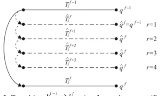
at time t f. The idea of the sequential function specification method using
( )
( )
(
)
( )
(
)
( )
(
)
( )
( )
(
)
1
1
1
*
0
*
0
* 1 *
0
1
, , , , , d d
1
, , , , d d
1
, , , , d , , , , d d
f
f f
f
f
f
t
f f
t Γ
t
f
t
t
f f f
t
B F t F x t t J x t t
C
J x t t F x t t
F x t t F x t S x t F x t t t
C
−
−
−
Γ
−
ξ ξ + ξ Γ =
ξ Γ +
C
Ω Ω
ξ Ω + ξ Ω
∫ ∫
∫ ∫
∫
∫
∫
Fig. 2. Transition tf−1→tf using future time steps (R=4)
In the sequential function specification method the sensitivity coefficients are used (c.f. matrix (18)). In order to determine them, the governing equations (4) are differentiated with respect
to the unknown heat flux
( )
,j j
q =q x t
at boundary point
and then [6, 8, 9, 10] ,
j
x ∈ Γ
( )
( )
( )
( ) ( ) ( )
( )
( )
( )
2
,
, :
d ,
, d
, 1,
: ,
0,
0 : , 0
j
j
j
j j
j j
j
Z x t
C T Z x t
t x
C T T x t
Z x t
T t
Z x t x x
x W x t
n x x
t Z x t
⎧ ∂
= λ∇
⎪ ∂
⎪ ∈Ω
⎪ ∂
−
⎪⎪ ∂
⎨
⎪ ∂ ⎧⎪ =
⎪ ∈Γ = −λ ∂ = ⎨
⎪ ⎪⎩ ≠
⎪ = =
⎪⎩ (20)
where
( )
( )
,, j
j
T x t Z x t
q
∂ =
∂
(21)
So, in the case considered the additional boundary-initial problems (20) for j=1, 2, ..., J should be solved.
In equation (20) the derivative of substitute thermal capacity with respect to temperature, this means dC(T)/dT appears.
3. Boundary element method
The basic problem (4) for the arbitrary assumed value of boundary heat flux q(x,t) and the additional problems (20) associated with the sequential function specification method have been solved using the boundary element method for 2D parabolic equations.
So, we consider the following equation
( )
( )
, 2( )
( )
: F x t , ,
x C T F x t R x t
t
∂
∈Ω = λ∇ +
∂
(22) where for primary problem (4): F(x, t)=T(x, t), R(x, t)=0 and
for additional problems (20): F(x,t)=Zj (x,t), R(x,t)=
dC(T)/dTZj (x, t)∂T(x, t)/∂t.
It should be pointed out that taking into account the course of functions C(T) and dC(T)/dT and the form of source functions appearing in additional problems, the equation (22) is strongly nonlinear. In order to solve it, the artificial heat source method has been applied [11, 12]. This method is a very effective supplementary algorithm first of all in a case of the BEM application for the non-linear problems solution.
We express the function C(T) as a sum of two components, this means a constant part C0 and a certain increment ΔC(T)
( ) 0 ( )
C T =C + ΔC T
(23)
The equation (22) can be written in the form
( )
2( )
( )
( )
( )
0
, ,
, ,
F x t F x t
C F x t R x t C T
t t
∂ = λ∇ + − Δ ∂
∂ ∂
(24) or
( )
2( )
( )
0
,
, ,
F x t
C F x t S x t
t
∂
= λ∇ +
∂ (25)
where
( )
,( )
,( )
F x t( )
,S x t R x t C T
t
∂ = − Δ
∂ (26)
is the artificial heat source term. The essential feature of equation (25) consists in a fact, that leaving out the last term we obtain the linear form of energy equation. Taking into account the possibilities of the boundary element method application in the range of non-steady problems modelling, this is a very convenient form of basic differential equation (a non-linearity appears only in the component determining the internal heat sources, and the function describing the fundamental solution for the problem considered is well known). The calculation of a source function requires, of course, the introduction of a certain iterative procedure [11, 12]. As was mentioned above, in order to solve the equation (25) the 1st scheme of boundary element method for 2D parabolic equations has been used. The boundary integral equation corresponding to the transition t f-1 → t f takes a form [13,14,15,16]
(27)
where ξ = ξ ξ
(
1, 2)
is the observation point, B( )
ξ =1 for ξ ∈ Ωand B
( ) ( )
ξ ∈ 0, 1 for is the fundamentalsolution [11, 12]
(
)
*
, , , ,f
F x t t
(
)
(
)
(
2)
* 1
, , , exp
4 4
f
f f
r
F x t t
a t t a t t
⎡ ⎤
⎢ ⎥
ξ = −
π − ⎢⎣ − ⎥⎦
(28)
where r is the distance between the points and x, a= λ/C0,
while J x t
( )
, = −λ∂F x t( )
, /∂n and(
)
*
, , ,f
J ξ x t t =
(
)
*
, , ,f / .
F x t t n
−λ ∂ ξ ∂
For constant elements with respect to time [13, 14], the equation (27) can be written in the form
( )
( )
( )
( )
( )
( )
(
) (
)
( ) ( )
* 1 1
, , , d
, , d
, , , , , , d
f f
f
f f f
B F t J x t g x
F x t h x
F x t t F x t S x t g x
Γ
Γ
− −
Ω
ξ ξ + ξ Γ =
ξ Γ +
⎡ ξ ξ ⎤
⎣
∫
∫
∫
⎦ Ω(29)
where
( )
(
)
1
*
0
1
, , ,
f
f
t
f
t
h x J x t t
C −
ξ =
∫
ξ , dt(30)
and
( )
(
)
1
*
0
1
, , ,
f
f
t
f
t
, d
g x F x t t
C −
ξ =
∫
ξ tj
(31) In order to solve equation (29), the boundary Γ is divided into N
constant boundary elements Γj, the interior Ω is divided into L constant internal cells Ωl and then we obtain the following system of algebraic equations (i=1, 2, ..., N)
(
)
(
)
(
)
(
)
1 1
1
1 1
, ,
, ,
N N
j f j f
i j i j
j j
L L
l f l f
i l i l
l l
G J x t H F x t
P F x t D S x t
= =
−
= =
= +
+
∑
∑
∑
∑
(32)
where
( )
, d and( )
, d ,1 / 2
j j
i j i
i j j i j
h x i
G g x H
i j
Γ Γ
⎧ ξ Γ ≠
⎪
= ξ Γ = ⎨
⎪− =
⎩
∫
∫
(33)
while
(
)
* 1
, , , d
l
i f f
i l l
P F x t t −
Ω
=
∫
ξ Ω(34)
at the same time
( )
, dl
i
i l l
D g x
Ω
=
∫∫
ξ Ω(35) After determining the 'missing' boundary values (F(x j, t f ) or
J(x j, t f )), the values of function F(x i, t f ) at internal nodes i
x ∈ Ω for time t f
are calculated using the formula (i=N+1, N+2, ..., N+L)
(
)
(
)
(
)
(
)
(
)
1
1
1
, ,
, ,
N
j f j f j f
i j i j
j
L
l f l f
i l i l
l
F x t H F x t G J x t
P F x t D S x t
=
−
=
,
⎡ ⎤
= ⎣ − ⎦+
⎡ + ⎤
⎣ ⎦
∑
∑
(36)
4. Results of computations
The lateral section of steel ingot 0.1×0.1[m] has been considered - c.f. Figure 1. The following input data have been assumed: thermal conductivity λ=35[W/mK], constant C0 =54.243⋅10 6 [J/m3 K] (c.f. equation (25)), liquidus temperature
TL =1505°C, solidus temperature TS =1470°C, pouring temperature T0 =1550°C, volumetric specific heats of liquid and
solid states cL =5.904⋅10
6
[J/m3 K], cS =4.875⋅10
6
[J/m3 K], volumetric specific heat of mushy zone sub-domain cP =0.5(cL +cS), volumetric latent heat L=1.9845⋅10
9
[J/m3], pulling rate w=0.0183 [m/s].
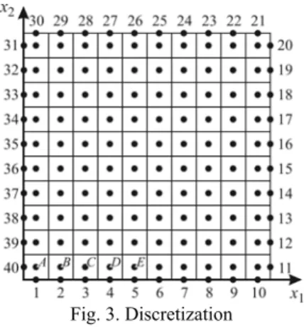
In Figure 3 the discretization of the domain considered is shown. The boundary is divided into 40 constant boundary elements, while the interior is divided into 100 constant internal cells. Time step equals Δt=0.25[s].
Fig. 3. Discretization
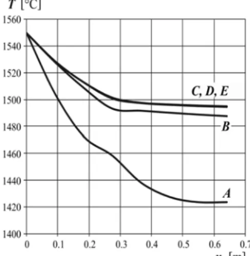
In order to estimate the course of boundary heat flux we assume, that the temperatures at the internal nodes A, B, C, D, E for successive cross sections x3 =fwΔt, f=0,1,...,14 of the cast
slab (c.f. Figure 1) are known. In Figure 4 the values of temperature at these nodes are shown. The information concerning the temperature distribution has been obtained from the direct problem solution under the assumption that the boundary heat flux changes according the formula
( )
1 2 ,q t = +b b t
References
The inverse problem has been solved using the sequentialfunction specification method for R=1, R=2 future time steps
and In Figure 5 the real course of
boundary heat flux and the identified heat flux are shown.
1 4
* 10 , 1, 2, ..., 5.
j
q = j=
[
1] B. Mochnacki, J. S. Suchy, Numerical Methods in Computations of Foundry Processes, PFTA, Cracow, 1995. Summing up, the sequential function specification methodcoupled with the boundary element method allows to identify the boundary heat flux.
[2] B. Mochnacki, J. S. Suchy, "Application of numerical methods for continuous casting process simulation", GIFA Congress, Official Exchange Paper, Dusseldorf, 1994. [3] E. Majchrzak, "Numerical simulation of continuous casting
solidification by boundary elements", Engineering Analysis with Boundary Elements, 11 (1993) 95-99.
[4] B. Mochnacki," Application of the BEM for numerical modelling of continuous casting", Computational Mechanics, 18, Springer-Verlag, pp. 55-61 (1996).
[5] W. Mikowicz, E. Sparrow, G. Schneider, H. Pletcher, Handbook of numerical heat transfer, J.Wiley & Sons, New York, 1988.
[6] K. Kurpisz, A. J. Nowak, Inverse thermal problems, CMP, Southampton, Boston, 1995.
[7] J. Mendakiewicz, Estimation of boundary heat flux during cast iron solidification, Scientific Research of the Institute of Mathematics and Computer Science of Czestochowa University of Technology, Czestochowa, 1(6) (2007) 191-198.
[8] R. Szopa, Sensitivity analysis and inverse problems in the thermal theory of foundry, Publ. of the Czest. Univ. of Techn., Czestochowa, 2006 (in Polish).
Fig. 4. Temperature at the points A, B, C, D, E
[9] J. Mendakiewicz, Inverse problem of solidification modelling - identification of substitute thermal capacity, Simulation, Designing and Control of Foundry Processes, Published by AGH University of Science and Technology, Kraków, 2006, 33-41.
[10] R. Szopa, S. Lara, Application of simplified model to sensitivity analysis of solidification process, Archives of Foundry Engineering, Vol. 7, 4 (2007) 169-174.
[11] E. Majchrzak, B. Mochnacki, "The BEM application for numerical solution of non-steady and non-linear thermal diffusion problems", Computer Assisted Mechanics and Engineering Sciences, Vol. 3, 4 (1996) 327-346.
[12] B. Mochnacki, E. Majchrzak, "Application of the BEM in thermal theory of foundry, Engineering Analysis with Boundary Elements, 16 (1995) 99-1215.
[13] P. K. Banerjee, Boundary element methods in engineering, McGraw-Hill Company, London, 1994.
[14] E.Majchrzak, Boundary element method in heat transfer, Publ. of the Tech. Univ. of Czest., Czestochowa, 2001. Fig. 5. Real and identified boundary heat fluxes
[15] E. Majchrzak, B. Mochnacki, G.Kaua, Shape sensitivity analysis in numerical modelling of solidification, Archives of Foundry Engineering, Vol. 7, 4 (2007) 115-120.
Acknowledgement
[16] A. Bokota, S. Iskierka, An analysis of the diffusion-convection problem by the BEM, Engineering Analysis with Boundary Elements, 15 (1995) 267-275.