Nº 502
ISSN 0104-8910
Nonparametric specification tests for conditional duration
models
Nonparametric specification tests for conditional
duration models
Marcelo Fernandes
Joachim Grammig
Getulio Vargas Foundation University of T¨ubingen
[email protected] [email protected]
Abstract:This paper deals with the testing of autoregressive conditional dura-tion (ACD) models by gauging the distance between the parametric density and hazard rate functions implied by the duration process and their non-parametric estimates. We derive the asymptotic justification using the functional delta method for fixed and gamma kernels, and then investigate the finite-sample properties through Monte Carlo simulations. Although our tests display some size distortion, bootstrapping suffices to correct the size without compromising their excellent power. We show the practical usefulness of such testing proce-dures for the estimation of intraday volatility patterns.
JEL Classification: C14, C41, C52.
Keywords: duration models, gamma kernel, hazard rate, specification testing.
Acknowledgements: We are indebted to three anonymous referees, Renato Flˆores, Søren Johansen, and many seminar participants for helpful comments, as well as to Sandra Vuleti´c and Bernardo de S´a Mota for valuable research assistance. Fernandes acknowledges with gratitude the financial support from CNPq-Brazil and a Jean Monnet Fellowship at the European University Insti-tute. The usual disclaimer applies.
1
Introduction
The availability of financial transactions data has raised the level of interest in applied microstructure research. Thinning raw data enables analysts to define the events of interest, e.g. quote updates and limit-order execution, and then compute the corresponding waiting times. Typically, the resulting duration pro-cesses are influenced by public and private information, which motivates the use of conditional duration models. Therefore, it is no wonder that microstructure studies employing conditional duration models abound in the literature (e.g. Lo, MacKinlay and Zhang, 2002). In particular, price durations (time between mar-ket maker’s mid-quote changes) are closely linked to the instantaneous volatility of the mid-quote price process (Engle and Russell, 1998) and thus they play an interesting role in option pricing (Prigent, Renault and Scaillet, 2001) and intra-day risk management (Giot, 2000). Trade and volume durations mirror in turn features such as market liquidity and the information arrival rate (Gouri´eroux, Jasiak and Le Fol, 1999).
Engle and Russell’s (1998) autoregressive conditional duration (ACD) model is the starting point of such analyses, though there are several extensions. Ghy-sels and Jasiak (1998), Engle (2000) and Grammig and Wellner (2002) com-bine conditional duration models with GARCH-type effects, whereas Ghysels, Gouri´eroux and Jasiak (2002) introduce a stochastic volatility duration model to cope with higher order dynamics in the duration process. Zhang, Russell and Tsay (2001) advocate a nonlinear version of the ACD model rooted in a self-exciting threshold autoregressive framework. Bauwens and Veredas (1999), Lunde (1999), Grammig and Maurer (2000), and Hamilton and Jorda (2001) argue for conditional duration models that accommodate more flexible hazard rate functions. Bauwens and Giot’s (2000) logarithmic ACD model provides a more suitable framework for testing market microstructure hypotheses as it avoids some of the parameter restrictions implied by the original ACD spec-ification. Fernandes and Grammig (2003) put forth a very flexible family of augmented ACD processes that nests most ACD models in the literature.
distribution of the error term (i.e. standardized duration) is correctly specified. Engle and Russell (1998) check the first and second moments of the residuals with particular attention to measuring excess dispersion, while others use QQ-plots (Bauwens and Veredas, 1999) and Bartlett identity tests (Prigent et al., 2001). Grammig and Wellner (2002) take a different approach by estimating and testing conditional duration models using a GMM framework. Bauwens, Giot, Grammig and Veredas (2000) employ the techniques developed by Diebold, Gunther and Tay (1998) to evaluate density forecasts of conditional duration models.
At first sight, misspecification of the distribution of the standardized du-ration may seem unimportant given that quasi maximum likelihood (QML) methods based on distributions belonging to the standard gamma family (with two parameters), such as the exponential, provide consistent estimates (Drost and Werker, 2003). However, QML estimation of conditional duration models may perform quite poorly in finite samples. Consider, for instance, a data gen-erating process with a nonmonotonic baseline hazard rate function. Estimation by QML using the exponential distribution fails to produce sound results even in quite large samples (Grammig and Maurer, 2000). Further, the misspecifica-tion of the baseline distribumisspecifica-tion has quite serious implicamisspecifica-tions for models that attempt to uncover the link between duration and volatility as in Ghysels and Jasiak (1998) and Engle (2000). Indeed, the success of option pricing and risk management procedures based on intraday volatility estimates from price du-ration models depends heavily on the appropriate specification of the baseline hazard rate function (Giot, 2000; Prigent et al., 2001).
(1995), Fan and Li (1996), Li (1996), Zheng (1996), and Fan and Ullah (1999). Our tests are not only simple, but also have some desirable properties. In contrast to Bartlett identity tests (Chesher, Dhaene, Gouri´eroux and Scaillet, 1999), they examine the whole distribution of the residuals instead of a small number of moment restrictions. In addition, our tests are nuisance parameter free in that there is no asymptotic cost in replacing the errors (i.e. standardized durations) with estimated residuals. Monte Carlo simulations moreover indicate that some versions of our tests entail excellent performance in terms of finite-sample size and power.
The remainder of this paper is organized as follows. Section 2 describes the family of conditional duration models we have in mind. Section 3 discusses the design of the testing procedures. Section 4 deals with the limiting behavior of such tests. First, we show asymptotic normality under the null hypothesis that the conditional duration model is properly specified. Second, we compute the asymptotic local power by considering a sequence of local alternatives. Third, we derive the conditions in which our tests are nuisance parameter free. Section 5 investigates finite-sample properties of the asymptotic and bootstrap-based variants of our tests through Monte Carlo simulations. Section 6 applies our testing procedures to assess the performance of the linear ACD model for Exxon price durations at the New York Stock Exchange (NYSE), so as to highlight the effects of misspecifying the baseline distribution on the instantaneous volatil-ity estimation. Section 7 summarizes the main results and offers concluding remarks. For ease of exposition, an appendix collects all proofs and technical lemmas.
2
Conditional duration models
Letzi =ψiǫi ≥0, where the duration zi =ti−ti−1 denotes the time elapsed
between events occurring at timetiandti−1, the conditional expected duration
process ψi = E
¡
zi|Ii−1 ¢
is independent of the standardized duration ǫi, and
Ii−1 is the set including all information available at time ti−1. To nest the
existing ACD models, we consider the following general specification for the conditional mean process
ψi =g(ψi−1, . . . , ψi−q, ǫi−1, . . . , ǫi−p, ui;φ), (1)
whereui|Ii−1∼N(0, σ2u) andφ is a vector of parameters. For instance, Engle
whereas Fernandes and Grammig (2003) assume the more flexible specification
ψiλ=ω+α ψλi−1 h¯
¯ǫi−1−b ¯
¯+c¡ǫi−1−b¢i
υ
+β ψiλ−1.
If the aim is to model microstructure effects, one can also incorporate additional predetermined variables (Engle and Russell, 1998; Bauwens and Giot, 2000).
Further, suppose that the standardized durationǫi is iid with Burr density
fB(ǫi, θB) =
κ ξκ Bǫκi−1
(1 +γ ξκ Bǫκi)
1+1/γ, (2)
whereθB= (κ, γ),κ > γ >0 and
ξB ≡
Γ¡1 + 1/κ¢Γ¡1/γ−1/κ¢
γ1+1/κΓ¡1 + 1/γ¢ . (3)
It is readily seen that the conditional density ofzi is also Burr with parameter
vector¡ξκ
Bψ−i κ, κ, γ
¢
. Accordingly, the conditional hazard rate function reads
HB¡zi
¯
¯Ii−1;θB
¢
= κ ξ
κ
Bψ−i κzκi−1
1 +γ ξκ Bψ−
κ i zκi
, (4)
which is nonmonotonic with respect to the standardized duration ifκ >1. Whenγshrinks to zero, (2) reduces to a Weibull distribution, viz.
fW(ǫi, θW) =κ ξκW ǫiκ−1exp (−ξWκ ǫκi), (5)
whereθW =κandξW = Γ(1 + 1/κ). Accordingly, the conditional distribution
of the duration process is also Weibull and the conditional hazard rate function reads HW¡zi
¯
¯Ii−1;θW
¢
= κ ξκ W ψ−
κ i z
κ−1
i . In contrast to the Burr case, the
conditional hazard rate implied by the Weibull distribution is monotonic. It decreases with the standardized duration for 0 < κ < 1, increases for κ > 1 and remains constant forκ= 1. In the latter case, the Weibull coincides with the exponential distribution and the conditional hazard rate function of the duration process is simplyHE¡zi
¯ ¯Ii−1
¢
=ψ−i1.
As an alternative, Lunde (1999) puts forward the generalized gamma ACD model, whereǫi is iid with density
fG(ǫi, θG) =
ξκγG κǫκγi −1
Γ(γ) exp (−ξ
κ
Gǫκi) (6)
whereθG = (κ, γ) andξG≡Γ(γ+ 1/κ)/Γ(γ). The generalized gamma
on the incomplete gamma integralI(ǫi, γ)≡
Rǫi
0 u
γ−1exp(−u) du. Nonetheless,
it is possible to derive its shape properties according to the parameter values (Glaser, 1980). Ifκγ <1, the hazard rate is decreasing forκ≤1, and U-shaped forκ >1. Conversely, ifκγ > 1, the hazard rate is increasing for κ≥1, and inverted U-shaped forκ <1. Lastly, ifκγ = 1, the hazard rate is decreasing for κ <1, constant forκ= 1 (exponential case), and increasing forκ >1.
Albeit Engle and Russell (1998) suggest the use of exponential and Weibull distributions, the Burr and the generalized gamma ACD models seem to de-liver better results for both price and trade durations (Lunde, 1999; Bauwens et al., 2000; Zhang et al., 2001). It remains the fact however that quasi maxi-mum likelihood estimates are consistent only if based on the standard gamma distribution with two parameters (Drost and Werker, 2003).
3
Specification tests
As conditional duration models are usually estimated by the (quasi) maximum likelihood method, likelihood ratio tests are available to compare nested dis-tributions in conditional duration models. However, due to the presence of inequality constraints in the parameter space, the limiting distribution of the test statistic is a mixing ofχ2−distributions with probability weights
depend-ing on the variance of the parameter estimates (Wolak, 1991). Accorddepend-ingly, it is extremely difficult to obtain empirically implementable asymptotically exact critical values. As an alternative, Wolak (1991) suggests applying asymptotic bounds tests, but bounds are usually quite slack, and are more likely to yield inconclusive results.
In the following, we design a testing strategy to check the parametric speci-fication of the distribution of the standardized durationǫi by matching density
functionals. More precisely, we assume that the conditional mean processψi is
correctly specified and then test whether there is any valueθ0 of the parameter
vector such that the true and parametric density functions of the standardized duration coincide almost everywhere. We first consider the general problem of testing the null
H0: ∃θ0∈Θ such that f(x, θ0) =f(x) (7)
against the alternative hypothesis that there is no suchθ0∈Θ for a nonnegative
random variableX with independent observations x1, . . . , xn. In our context,
role of the nonnegative random variable X, is unobservable. We thus extend the results in Section 4.4 to testing the estimated residuals of the conditional duration modelbǫi=zi/ψbi (i= 1, . . . , n).
The true cumulative distribution function F of the standardized durations and the density f are of course unknown, otherwise we could merely verify whether they belong to the specified parametric family of distributions. Ac-cordingly, we estimate the density function using kernel methods, so as to have consistent estimates irrespective of the parametric specification of the distribu-tion. Because the parametric density estimator is consistent only under the null, it is natural to develop tests that gauge the closeness between these two density estimates.
Our first testing procedure, which we label the D-test, rests on measuring the following distance
Φf =
Z
x
I(x∈ S)£f(x, θ)−f(x)¤2dF(x), (8) whereRxdenotes the integral over the support of the density function ofxand
I(·) is the indicator function. The distance (8) weighs the difference between the parametric and nonparametric estimators according to their relevance as measured by the density function. Further, it is nonnegative with equality holding if and only iff(x) coincides withf(x, θ) for everyx∈ S. We introduce the subsetS so as to avoid regions in which density estimation is unstable.
The sample analog of (8) reads
Φfˆ=
1 n
n
X
i=1
I(xi ∈ S)
h
f¡xi,θˆ
¢
−fˆ(xi)
i2
, (9)
where ˆθ and ˆf(·) denote pointwise consistent estimates of the true parameter θ0 and density f(·), respectively. The null hypothesis is then rejected if the
D-test statistic Φfˆis large enough. One could also work with other measures
of closeness such as the integrated (rather than mean) square difference as in Bickel and Rosenblatt (1973) and Fan (1994).
By virtue of the one-to-one mapping linking hazard rate and density func-tions, the null hypothesis (7) implies that there exists aθ0 ∈ Θ such that the
hazard rate function implied by the parametric model Hθ0(·) equals the true
hazard functionHf(·). Accordingly, we consider a second test, which we refer to as the H-test, relying on the statistic
Λfˆ=
1 n
n
X
i=1
I(xi∈ S)
h
Hθˆ(xi)− Hfˆ(xi)
i2
whereHθˆandHfˆare the parametric and nonparametric estimates of the
base-line hazard rate function, respectively. From the discussion above, (10) is close to zero under the null, while it is large under the alternative.
The next section shows that the limiting distribution of the D- and H-test statistics do not depend on how one estimates the parametric density func-tion. This follows from the fact that the nonparametric density estimation converges at a slower rate than the parametric density estimation. One could therefore employ maximum likelihood methods. Alternatively, to provide a minimum-distance flavor to the D- and H-tests, one can estimate the paramet-ric density by minimizing (9) and (10), respectively. The resulting estimators ˆ
θD
n ≡argminθ∈ΘΦfˆand ˆθHn ≡argminθ∈ΘΛfˆbelong to the class of M-estimators
discussed by Newey (1994) as they hinge on a two-step procedure in which the first step involves a kernel estimation and the second step solves a minimization problem.
4
Asymptotic justification
In what follows, we derive asymptotic results for the test statistics and their implied M-estimators. In fact, the limiting behavior of the D-test was already investigated by A¨ıt-Sahalia (1996), who extends Bickel and Rosenblatt’s (1973) framework to estimate and test diffusion processes. Accordingly, the assump-tions we impose are quite similar and the asymptotic results are the same up to a weighting scheme.
4.1
Assumptions
Letx1, . . . , xn denote independent observations on a random variable X with
probability density functionf(x),x∈[0,∞). We consider the following set of regularity conditions.
A1 The density functionf is continuously differentiable up to orders+ 1 and its derivatives are bounded and square integrable. Further,f is bounded away from zero on the compact intervalS.
A2 The fixed kernelKis of orders(even integer) and is continuously differen-tiable up to ordersonRwith derivatives inL2(R). Lete
K ≡RuK2(u) du
andvK ≡
R
v
£R
uK(u)K(u+v) du
¤2
A3 As the sample size n grows, the bandwidths for the fixed and gamma kernels are such thathn=o¡n−1/(2s+1)¢andbn=o¡n−4/9¢, respectively.
A4 The parameter space Θ⊂Rkis compact. Letζ(·, θ) denote the parametric density functionf(·, θ) for the D-test and the baseline hazard rate function
H(·, θ) for the H-test. In a neighborhood of the true parameterθ0,ζ(·, θ) is
twice continuously differentiable inθwith uniformly bounded second-order partial derivatives and the matrixE£∂
∂θζ(·, θ) ∂ ∂θ′ζ(·, θ)
¤
has full rank.
A5 Consider f∗ and f+ in a neighborhood Nf of the true density f. Then,
the leading termϑf that drives the asymptotic distribution of the implied
M-estimators is such that
(i) E|ϑf|3+r<∞, for somer >(3 +η)(3 +η/2)/ηandη >0
(ii) E sup
f∗∈Nf
|ϑf∗| 2<
∞
(iii) E|ϑf∗−ϑf+|
2
≤ckf∗−f+kL(∞,m),
wherecis a constant,k·kL(∞,m)denotes the Sobolev norm of order (∞, m)
andmis an integer such that 0< m < s/2 + 1/4.
Assumption A1 requires that the density function is smooth enough to admit a functional Taylor expansion. Although assumption A2 provides enough room for higher-order kernels, in what follows, we implicitly assume that the kernel is of second order (s= 2) as in Hall (1984). In particular, we will focus attention on Ghosh and Huang’s (1991) optimal uniform kernel for whicheK = (2
√
3)−1and
vK = (3 √
3)−1. Assumption A3 induces undersmoothing in order to simplify the
asymptotic bias of the test statistics. The optimal rate would imply additional bias terms as in Fan (1994). Assumption A4 guarantees that the functionalsθD f
andθH
f implied by the M-estimators are well defined. Lastly, it follows from A5
that one can consistently estimate the asymptotic variance of the M-estimators using a nonparametric correction `a la Newey and West (1987).
4.2
Matching the density function
The D-test gauges the discrepancy between the parametric and nonparametric estimates of the density function. It follows from (9) that the functional of interest is
Φfˆ= Z
x
I(x∈ S)hf(x, θfˆ)−fˆ(x) i2
where θfˆis the functional implied by the estimator of θ and Fn denotes the
empirical cumulative distribution function. Assume further that it admits the following (von Mises) functional expansion
Φfˆ= Φf+ DΦf(hx) +
1 2D
2Φ
f(hx, hx) +O
¡
khxk3¢, (12)
where hx =h(x) = ˆf(x)−f(x) and k · kdenotes theL2 norm. By the Riesz
representation theorem, the functional derivative DΦf(·) has a dual
representa-tion of the form DΦf(hx) =
R
xψf(x)hxdx. It follows from A¨ıt-Sahalia’s (1994)
functional delta method that ψf stands for the leading term that drives the
asymptotic distribution of Φfˆ. If the first functional derivative is degenerate,
then the asymptotic distribution is driven by the second-order term of the ex-pansion. See also von Mises (1947), Serfling (1980), and Ren and Sen (2001).
Letfx andfx,θ denote the true and parametric density functions evaluated
atx, respectively. The first functional derivative of Φf reads
DΦf(hx) =
Z
S
(fx,θ−fx)2hxdx+ 2
Z
S
·
∂fx,θ
∂θ Dθf(hx)−hx
¸
(fx,θ−fx)fxdx,(13)
where Dθf(·) denotes the first derivative of the functionalθfimplied by the QML
estimator. As DΦf(hx) is singular under the null, the limiting distribution of
Φfˆdepends on the second functional derivative, namely
D2Φf(hx, hx) = 2
Z
S
∂f(x, θf)
∂θ
∂f(x, θf)
∂θ′
£
Dθf(hx)¤2fxdx
−4
Z
S
∂f(x, θf)
∂θ Dθf(hx)fxhxdx+ 2
Z
S
fxh2xdx. (14)
However, the first and second terms of the right-hand side do not affect the asymptotic distribution of the test statistic. A¨ıt-Sahalia (1994) shows indeed that the asymptotics are driven by the unsmoothest term of the first nondegen-erate derivative because it converges at a slower rate. The third term contains a Dirac mass in its inner product representation, and thus leads the asymptotics.
Proposition 1. Under the null and assumptions A1 to A4, the statistic
b
τnD=
nh1n/2Φfˆ−h−n1/2δbD
b
σD
d
−→N(0,1), (15)
wherebδDandbσD2 are respectively consistent estimates ofδD≡eKE£I(x∈ S)fx¤
andσ2
D≡vKE
£
I(x∈ S)f3
x
¤
.
To obtain consistent estimates of δD and σD2, one may use the empirical
distribution to compute the expectation and plug in the corresponding kernel density estimate, then yielding
b
δD = eK 1
n
n
X
i=1
I(xi∈ S) ˆf(xi)
b
σD2 = vK
1 n
n
X
i=1
I(xi∈ S)
£ˆ
f(xi)
¤3
.
As the time elapsed between transactions is strictly positive, durations have a support which is bounded from below. Further, the bulk of duration data is typically in the vicinity of the origin. Accordingly, the test statistic bτD
n may
perform poorly due to the boundary bias that haunts nonparametric estimation using fixed kernels. One solution is to work with log-durations whose support is unbounded and density is easily derived. Indeed, ifY = logX, thenfY(y) =
fX
£
exp(y)¤exp(y). An alternative rests on estimating the density function using asymmetric kernels to benefit from the fact that they never assign weight outside the density support (see Bouezmarni and Rolin, 2001, Bouezmarni and Scaillet, 2002, Chen, 1999 and 2000, Scaillet, 2003). In particular, the gamma kernel
Kx/bn+1,bn(u) =
ux/bnexp(−u/b
n)
Γ(x/bn+ 1)bx/bn n+1
I(u≥0) (16)
with bandwidthbn provides estimates that are consistent, nonnegative,
bound-ary bias free, and achieve the optimal rate of convergence for the mean inte-grated error for any density function whose support is bounded from the origin (Bouezmarni and Scaillet, 2002; Chen, 2000). We therefore consider a second version of the D-test in which the density estimation uses a gamma kernel.
Proposition 2. Under the null and assumptions A1 to A4, the statistic
˜ τnD=
nb1n/4Φf˜−b−n1/4δ˜G
˜ σG
d
−→N(0,1), (17)
whereδ˜G andσ˜2G are consistent estimates ofδG= 2√1πE
£
I(x∈ S)x−1/2f
x
¤
and
σ2
G= √12πE
£
I(x∈ S)x−1/2f3
x
¤
, respectively.
As above, consistent estimates ofδGandσG2 are readily available by plugging
in the empirical distribution and gamma kernel density estimate ˜f, viz.
˜ δG =
1 2√πn
n
X
i=1
˜ σG2 =
1 √ 2πn n X i=1
I(xi ∈ S)x−i 1/2
£˜
f(xi)¤3.
Consider now, as in A¨ıt-Sahalia, Bickel and Stoker (2001), the sequence of local alternatives
HD
1n: sup
x∈S
¯ ¯
¯f[n](x, θ)−f[n](x)−ε
nℓD(x)
¯ ¯
¯=o(εn), (18)
where°°f[n]−f°°=o¡ε2
n
¢
and
εn=
½
n−1/2h−1/4
n when using a fixed kernel
n−1/2b−1/8
n when using a gamma kernel.
(19)
Assume further that ℓD(x) is such that ℓSD ≡ E
£
I(x ∈ S)ℓ2
D(x)
¤
exists and E£ℓD(x)
¤
= 0. The next result illustrates the fact that both versions of the D-test have nontrivial power under local alternatives that shrink to the null at the corresponding rateεn.
Proposition 3. Under the sequence of local alternatives HD
1n and assumptions
A1 to A4,τbnD d
−→N¡ℓSD/σD,1
¢
, whereasτ˜nD d
−→N¡ℓSD/σG,1
¢
.
To maximize the power of both versions of the D-test, one could consider the most favorable scenario to the parametric model by utilizing the M-estimator ˆ
θD
n. The corresponding implicit functional then is
Z
S
∂f¡x, θD f
¢
∂θ
£
f¡x, θDf
¢
−f(x)¤ f(x) dx≡0, (20)
which produces
DθfD(hx) =
½Z
S
∂f(x, θ) ∂θ
∂f(x, θ)
∂θ′ f(x) dx
¾−1Z
S
∂f(x, θ)
∂θ f(x)h(x) dx. (21)
Accordingly, the limiting distribution is driven by
ϑD
f(x) =I(x∈ S)
½Z
S
∂f(x, θ) ∂θ
∂f(x, θ)
∂θ′ f(x) dx
¾−1
∂f(x, θ)
∂θ f(x). (22)
Proposition 4. Under the null and assumptions A1 to A4,n1/2¡θˆDn −θ0 ¢ d
−→
N(0,ΩD), whereΩD≡P∞k=−∞Cov
h
ϑD
f(xi), ϑDf(xi+k)
i
is the long run
covari-ance matrix of ϑD
f. In addition, if assumption A5 holds, it suffices to plugθˆDn
intoϑD
f and truncate the infinite sum as in Newey and West (1987) to obtain
a consistent estimator of the asymptotic variance.
4.3
Matching the baseline hazard rate function
The H-test compares the parametric and nonparametric estimates of the baseline hazard rate. The motivation is simple. The usual densities associated with duration models may engender fairly similar shapes depending on the parameter values. In turn, they hatch very different hazard rate functions: flat for the exponential, monotonic for the Weibull and nonmonotonic for the Burr and the generalized gamma distributions.
From (10), the functional of interest reads
Λfˆ = Z ∞
0
I(x∈ S)£Hθ(x)− Hfˆ(x) ¤2
dFn(x)
=
Z
S
£
Hθ(x)− Hfˆ(x)¤2dFn(x), (23)
Suppose that (23) admits a second-order Taylor expansion about the true den-sity, viz.
Λfˆ= Λf+ DΛf(hx) +
1 2D
2Λ
f(hx, hx) +O
¡
khxk3¢, (24)
where Λf =RS£Hθ(x)−Hf(x)¤2f(x) dxandhx=h(x) = ˆf(x)−f(x) as before.
The first functional derivative is then
DΛf(hx) =
Z
S
£
Hθ(x)− Hf(x)¤2hxdx
+ 2
Z
S
£
Hθ(x)− Hf(x)¤
·
∂Hθ(x)
∂θ Dθf(hx)−DHf(hx)
¸
dF(x),(25)
where
DHf(hx) =
h(x)− Hf(x)RuI(u < x)h(u) du Sx
(26)
and Sx denotes the survival function 1−F(x). It is readily seen that, if the
baseline hazard is properly specified, the first derivative is singular.
The asymptotic distribution of the H-test relies then on the second order functional derivative, which under the null reads
D2Λf(hx, hx) = 2
Z
S
£
DHf(hx)
¤2
dF(x)
+ 2
Z
S
∂Hθ(x) ∂θ
∂Hθ(x)
∂θ′ [Dθf(hx)]
2dF(x)
−4
Z
S
∂Hθ(x)
∂θ Dθf(hx)DHf(hx) dF(x). (27)
Proposition 5. Under the null and assumptions A1 to A4, the statistic
b
τnH=
nh1n/2Λfˆ−h−n1/2λbH
b
ςH
d
−→N(0,1), (28)
where bλH and bςH2 are consistent estimates of λH =eKE
£
I(x ∈ S)Hf(x)/Sx
¤
andς2
H =vKE£I(x∈ S)H3f(x)/Sx¤, respectively.
To obtain consistent estimates of λH and ςH2, one may compute the
expec-tation using the empirical distributionFn and plug in the corresponding kernel
estimates ˆf andFb of the density and cumulative distribution functions to esti-mate the hazard rate and survival functions. This yields
b
λH = eK
1 n
n
X
i=1
I(xi ∈ S) ˆf(xi)
£
1−F(xb i)
¤−2
b
ς2
H = vK
1 n
n
X
i=1
I(xi∈ S)
£ˆ
f(xi)
¤3£
1−Fb(xi)
¤−4
.
Other nonparametric estimators for the hazard rate and survival functions could also be used. See Ramlau-Hansen (1983), Nielsen (1998), and Nielsen and Tang-gaard (2001).
In contrast to the density function, in general, there is no closed form solution for the hazard rate of the log-standardized duration. One may of course solve it by numerical integration, though at the expense of simplicity. Notwithstanding, it is straightforward to fashion the H-test to gamma kernels.
Proposition 6. Under the null and assumptions A1 to A4, the statistic
˜ τH
n =
nb1n/4Λf˜−b−n1/4λ˜G
˜ ςG
d
−→N(0,1), (29)
where ˜λG and ς˜G2 estimate consistently λG = 2√1πE
£
I(x∈ S)x−1/2Hf(x)/S
x
¤
andς2
G= √12πE
h
I(x∈ S)x−1/2H3
f(x)/Sx
i
, respectively.
Again, consistent estimates ofλG andςG2 follows by plugging in the gamma
kernel density and cumulative distribution estimates ˜f and ˜F, giving way to
˜ λG =
1 2√πn
n
X
i=1
I(xi∈ S)x−i 1/2f(x˜ i)
£
1−F˜(xi)
¤−2
˜ ςG2 =
1 √ 2πn n X i=1
I(xi∈ S)x−i 1/2
£˜
f(xi)
¤3£
1−F(x˜ i)
¤−4
.
Consider next the following sequence of local alternatives
H1Hn: sup x∈S
¯ ¯
¯H[n](x, θ)− Hf[n](x)−εnℓH(x)
¯ ¯
where °°H[fn]− Hf
°
° = o¡ε2
n
¢
and ℓH(x) is such that ℓSH ≡E
£
I(x∈ S)ℓ2
H(x)
¤
exists andE£ℓH(x)
¤
= 0. It then follows that both versions of the H-test can distinguish alternatives that get closer to the null at the corresponding rateεn
in (18) while keeping the power constant.
Proposition 7. Under the sequence of local alternatives HH
1n and assumptions
A1 to A4,τbH n
d −→N¡ℓS
H/ςH,1
¢
, whereasτ˜H n
d −→N¡ℓS
H/ςG,1
¢
.
Finally, consider the M-estimator ˆθH
n that minimizes the distance between
the parametric and nonparametric estimates of the baseline hazard rate func-tion. The corresponding implicit functional is
Z
S
∂H¡x, θH f
¢
∂θ
£
H¡x, θHf
¢
− Hf(x)¤ dF(x)≡0, (31)
which results in the following first functional derivative
DθfH(hx) =
½Z
S
∂H(x, θ) ∂θ
∂H(x, θ) ∂θ′ dF(x)
¾−1Z
S
∂H(x, θ)
∂θ DHf(hx) dF(x).(32)
From (26), it is readily seen that
ϑHf (x) =I(x∈ S)
½Z
S
∂H(x, θ) ∂θ
∂H(x, θ) ∂θ′ dF(x)
¾−1
∂H(x, θ)
∂θ Hf(x) (33)
is the leading term that drives the asymptotic distribution of the estimator.
Proposition 8. Under the null and assumptions A1 to A4, n1/2¡θˆH n −θ0
¢ d −→
N(0,ΩH), whereΩH ≡P∞k=−∞Cov
h
ϑH
f(xi), ϑHf(xi+k)
i
is the long run
covari-ance matrix of ϑH
f . In addition, provided that assumption A5 holds, it suffices
to plugθˆH
n intoϑHf and truncate the infinite sum as in Newey and West (1987)
to obtain a consistent estimator of the asymptotic variance.
4.4
Nuisance parameter freeness
All results so far consider testing the distributional properties of a random vari-ableX with independent observationsx1, . . . , xn. In the context of conditional
duration models, the interest is in testing the standardized durationsǫi=zi/ψi,
i= 1, . . . , n. However,{ǫi}is unobservable and the testing procedure must then proceed using the estimated residualsbǫi=zi/ψbi,i= 1, . . . , n. In the following,
we derive the conditions under which the D- and H-tests are nuisance parameter free, and hence there is no asymptotic cost in substituting residuals for errors.
To simplify notation, letei=ei(φ0) =zi/ψi(φ0) andbei=ei(φ) =b zi/ψi(φ),b
Engle and Russell (1998) show that this last assumption holds for the QML estimator based on the exponential distribution. We hereinafter assume that the regularity conditions ensuring the consistency and asymptotic normality of the QML estimation hold, including the correct specification of the conditional mean process given by (1). See Gallant and White (1988) and Lee and Hansen (1994) for in-depth discussions of those conditions. Alternatively, one could either employ semiparametric techniques as in Drost and Werker (2003) or follow a GMM estimation strategy as in Grammig and Wellner (2002).
Proposition 9. Under assumptions A1 to A4, the D- and H-tests are nuisance
parameter free in that there is no asymptotic cost in substituting the root−n
consistent estimatesǫbi’s for the unobservedǫi’s.
5
Numerical results
In this section, we conduct a limited Monte Carlo exercise to assess the perfor-mance of our tests in finite samples. The motivation rests on the fact that most nonparametric tests entail substantial size distortions in finite samples. For in-stance, Fan and Linton (2003) demonstrate how neglecting higher order terms that are close in order to the dominant term may provoke such distortions. Not surprisingly, we show that size distortions are indeed material, so that we also consider bootstrap-based versions of our tests as in Fan (1995) and Li and Wang (1998). As singled out by Horowitz and Savin (2000), bootstrapping permits the computation of meaningful size-corrected critical values, putting power figures into perspective. The results show that applying the standard bootstrap pro-cedure to the estimated residuals (Horowitz, 2001, Section 4.1.1) works pretty well, eliminating size distortions without compromising the power of the tests.
We generate 15,000 realizations of a linear ACD(1,1) model, i.e.
ψi =ω+α zi−1+β ψi−1, (34)
by drawing the errorsǫi =zi/ψi from four distributions: exponential, Weibull
withκ= 0.6, Burr withκ= 1.3 andγ= 0.4, and the generalized gamma with κ = 0.5 and γ = 3. We set α = 0.1 and β = 0.7 to match the typical esti-mates found in empirical applications. Further, we normalize the unconditional expected duration to one by imposing ω = 1−(α+β) and then set ψ0 = 1
ef-fects. These are typical sample sizes for data on trade and price durations, respectively. All results are based on 1,000 Monte Carlo replications.
For each replication and data generating process, we first compute QML estimates using the exponential distribution. The optimization procedure takes advantage of Han’s (1977) sequential quadratic programming algorithm, so as to accommodate general inequality constraints. Next, we examine the outcomes of our five tests: the D- and H-tests with Ghosh and Huang’s (1991) optimal uniform kernel and Chen’s (2000) gamma kernel applied to the residuals and the D-test with the optimal uniform kernel applied to log-residuals. We select the bandwidths by adjusting Silverman’s (1986) rule of thumb. The normal distribution serves as reference only for the log-standardized durations, the ref-erence being the exponential otherwise. Bearing assumption A4 in mind, we also divide the rule-of-thumb bandwidths by logn. For instance, the resulting bandwidth for the gamma kernel is
bbn= 1
logn
³ b
λ/4´−1/5³2−bλ´−4/5 n−4/9,
whereλbis some consistent estimator of the exponential parameter λ, e.g., the inverse of the sample mean.
The frequency of rejection of the null hypothesis is then computed in order to evaluate the size and power of the six tests. More precisely, size distortions are investigated by looking at all instances in which the estimated model nests the true specification, e.g. the likelihood considers a Burr density, though the true distribution is exponential. Conversely, to investigate the power of these tests, we examine situations in which the estimated model does not encompass the true specification, e.g. the estimated model specifies an exponential distribution, whereas the true density is a Burr.
Figures 1 to 4 display the main results for n = 3,000 using Davidson and MacKinnon’s (1998) graphical representation to illustrate the finite-sample properties of the asymptotic and bootstrap-based tests for the ACD process with exponential, Weibull, Burr and generalized gamma errors, respectively.1
Each figure consists of two columns of charts. The first column corresponds to the asymptotic tests, whereas the second column illustrates the results for the bootstrap-based tests with 499 artificial samples. For every chart, the horizon-tal axis represents the significance level, while the vertical axis represents the
1
probability of rejection at that level. Ideally the size of a test, i.e. the probabil-ity of rejection under the null, coincides with the significance level, whereas the power, i.e. the probability of rejection under the alternative, is close to one.
The asymptotic tests based on the optimal uniform kernel exhibit substan-tial size distortions unless applied to the log-residuals for which it is slightly liberal irrespective of the data generating process. Bootstrapping the estimated residuals however suffices to correct the size of the tests without affecting their power. In contrast, the asymptotic gamma-based tests perform relatively well both in terms of size and power, hence bootstrapping is not really necessary. As is apparent, our tests exhibit excellent power unless one wishes to distinguish between the generalized gamma and Burr distributions. The H-test with opti-mal kernel has the worst performance: It almost never rejects the Burr ACD specification when the true baseline distribution is the generalized gamma.
For the sake of comparison, we also run the overdispersion test as advo-cated by Engle and Russell (1998) for the ACD models with the exponential and Weibull distributions. The performance of the overdispersion test is quite disappointing. Figures 1 and 2 show that, despite its parametric nature, size distortions are material as also evinced by Chesher et al. (1999). Although boot-strapping successfully corrects the size of the overdispersion test, Figures 3 and 4 make evident that its power performance is surprisingly poor relative to the nonparametric tests. Altogether, the D- and H- tests with gamma kernel seem to entail the best overall performance, though the D-test for log-standardized durations is a fair alternative, especially if one wishes to avoid bootstrapping.
6
Empirical application
In this section, we use NYSE price duration data to assess the performance of the linear ACD model (34) with exponential, Weibull, Burr, and generalized gamma distributions employing the testing framework outlined in Section 3. Exxon price durations from NYSE’s Trade and Quote (TAQ) database were kindly provided by Luc Bauwens and Pierre Giot, who thoroughly describe the data in Bauwens and Giot (1998 and 2000) and Giot (2000).
defined by thinning the quote process with respect to a minimum change in the mid-price of the quotes. We define price duration as the time interval needed to observe a cumulative change in the mid-price of at least $0.125 as in Giot (2000). Durations between events recorded outside the regular opening hours of the NYSE as well as overnight spells are removed.
As documented by Giot (2000), price durations feature a strong time-of-day effect related to predetermined market characteristics such as trade opening and closing times and lunch time for traders. We thus consider seasonally adjusted price durations zi = Zi/̺(ti), where Zi is the raw price duration in seconds
and ̺(·) denotes a intraday seasonal factor. As in Engle and Russell (1998), we estimate the latter by averaging durations over thirty-minute intervals for each day of the week and fitting a cubic spline with nodes at each half hour.2
The resulting (seasonally adjusted) price durations zi then serve as input for
the analysis.
The sample ranges from September to November 1996, consisting of 2,717 price durations. We use the first two thirds of the sample for estimation pur-poses, and reserve the remainder of the data to out-of-sample analysis. The descriptive statistics reported in Table 1 evince that Exxon price durations ex-hibit the two features that motivate ACD modeling: highly significant serial correlation and overdispersion.
6.1
Estimation results
We invoke (quasi) maximum likelihood methods to estimate the linear ACD model (34) with exponential, Weibull, Burr, and generalized gamma distribu-tions. More precisely, as advanced in Section 5, we first compute the QML estimates using the exponential distribution. This yields
ψi = 0.065 + 0.046zi−1+ 0.890ψi−1, (35)
(0.037) (0.016) (0.048)
where figures in parentheses refer to QML standard errors. We next obtain the series of residuals and one-step ahead forecast errors by forming both in- and out-of-sample standardized durationszi/ψbi.
Under the correct specification of the conditional mean, the residuals and forecast errors from (35) are both serially independent. We therefore check
2
Alternatively, one could employ Veredas, Rodriguez-Poo and Espasa’s (2001) semipara-metric approach to simultaneously estimate the seasonal component̺(·) and the parameters
whether the in- and out-of-sample residuals are serially independent by the means of the BDS test (Brock, Dechert, Scheinkman and LeBaron, 1996). In contrast to the Ljung-Box statistic, the BDS test is sensitive not only to serial correlation but also to other forms of serial dependence. Moreover, the BDS test is nuisance parameter free for additive models (de Lima, 1996), which is quite convenient given that we are testing estimated residuals rather than true errors. A simple log-transformation renders the linear ACD model additive, hence we work with the log-standardized durations. The results indicate that we cannot reject the null hypothesis of serial independence of the residuals and forecast errors at the 5% level of significance.3 The linear ACD specification thus seems
to do a pretty good job of accounting for the serial dependence of the Exxon price durations.
As the findings indicate that (35) is a congruent model, we can use the resid-uals to estimate by maximum likelihood the parameters of the Weibull, Burr and generalized gamma distributions. We find the following pointwise estimates (with their respective standard errors in parentheses): bκ= 0.962 (0.016) for the Weibull,bκ= 1.239 (0.042) and bγ = 0.432 (0.061) for the Burr, and bκ= 0.318 (0.056) andbγ= 8.052 (2.733) for the generalized gamma distribution. An infor-mal likelihood comparison based on the usual information criteria rejects both the exponential and the Weibull ACD models, thus justifying the flexibility brought about by the Burr and generalized gamma formulations.
6.2
Test results
To further evaluate the performance of the four linear ACD specifications, we employ the testing procedures put forth in Section 3 to their estimated residuals and one-step ahead forecast errors. Although we also report the p-values for the asymptotic D-test with optimal uniform kernel for the log-residuals, we focus attention to the bootstrap versions of our tests. We refrain from reporting the results of the H-test with optimal uniform kernel because, as seen in Section 5, it entails a very poor small-sample performance (even after bootstrapping). Finally, as advocated by Engle and Russell (1998), we also use the asymptotic and bootstrap-based overdispersion tests to check the exponential and Weibull specifications. As in Section 5, all bootstrap variants of the tests consider 499 artificial samples to build the empirical distribution of the test statistic.
3
Table 2 reports the in- and out-of-sample results, which grant support only to the linear ACD model with the generalized gamma distribution. The other ACD specifications are less successful. The bootstrap-based tests indeed reject the exponential and Weibull ACD models in all instances. In contrast to the asymptotic D-test for log-standardized durations, whose results conform with the evidence given by the bootstrap-based tests, the asymptotic overdispersion test fails to reject the exponential and Weibull specifications for the forecast errors. This illustrates how misleading the overdispersion test can be if one simply ignores the fact that, in small samples, it features size distortions.
Interestingly, we find mixed results for the Burr ACD model both in- and out-of-sample. As opposed to the D- and H-tests with gamma kernel, the asymptotic and bootstrap-based variants of the D-test for log-standardized durations are unable to reject the Burr distribution for the residuals and forecast errors at the 5% level of significance. This result is likely to exemplify the lack of power of the D-test for log-standardized durations to distinguish the generalized gamma from the Burr distribution.
6.3
Intraday volatility estimates
To better illustrate the consequences of misspecifying the innovation distribu-tion, we estimate the instantaneous volatility implied by our four specifications along the lines of Engle and Russell (1998). The instantaneous volatilityσ(t) is such that
σ2(t) = lim
∆t→0
1 ∆tE
·
P(t−∆t)−P(t) P(t)
¸2
. (36)
As we are interested in price durations, we can hold the price changecconstant and then take the limit in (36) to estimate the instantaneous volatility by means of the linear ACD model. More specifically,
σ2(t) =¡c/P(t)¢2H¡t/̺(t)¢̺(t). (37)
whereH(·) denotes the conditional hazard function implied by the ACD spec-ification and̺(t) corresponds to the seasonal component. Because the hazard function is defined for allt > t0, it is possible to draw a continuous picture of
the volatility over the trading day. As in Engle and Russell (1998), we compute annualized instantaneous volatilities by multiplyingσ2(t) by the annual trading
time in seconds.4 4
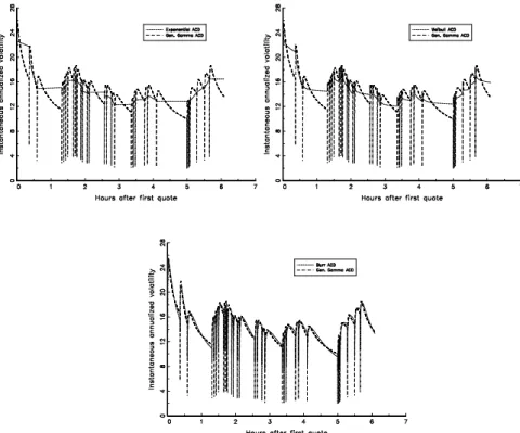
Figure 5 displays the instantaneous volatility estimates implied by each of the four ACD specifications for a typical trading day (Thursday, September 9, 1999). As the model selection procedure indicates that the generalized gamma ACD model is the best specification, the charts take its volatility estimates as reference in order to highlight the differences between the volatility estimates given by the other linear ACD models. As in Engle and Russell (1998), the spikes indicate event arrival times (quote changes), and the overall U-shaped volatility pattern over the course of the day confirms the previous findings in the intraday volatility literature (see, for example, Andersen and Bollerslev, 1997).
The variation of the instantaneous volatility implied by the exponential ACD model after the quote event in Figure 5 does not contradict the fact that the hazard rate function of the exponential distribution is flat. This is just a conse-quence of the seasonality of the quote intensity process. Asbκis slightly smaller than one, the instantaneous volatility implied by the Weibull ACD model is very similar to those implied by the exponential specification, though it mono-tonically decreases after a quote update. In contrast, the Burr and generalized gamma parameter estimates are such that their respective hazard function rates are nonmonotonic. Therefore, as implied by (37), it is not surprising that their implied instantaneous volatility estimates vary nonmonotonically after quote updates. Indeed, after a quote event, the instantaneous volatility seems to first decrease substantially, and then to sharply increase. It is worth noting that the generalized gamma specification predicts a much steeper slope than the Burr.
To sum up, the specifications with Weibull, Burr and generalized gamma baseline distributions all predict that it is most likely to observe a price event immediately after another price event. However, the intraday volatility esti-mates implied by the Weibull notably differ from those implied by the Burr and generalized gamma specifications. The instantaneous volatility decreases much faster for the Burr and generalized gamma than for the Weibull ACD model. This sort of instantaneous volatility pattern is consistent with the theoretical implications of Admati and Pfleiderer’s (1988) and Easley and O’Hara’s (1992) market microstructure models.
7
Concluding remarks
haz-ard rate function of standhaz-ardized durations. Asymptotic theory is derived for nonparametric density estimation using both fixed and gamma kernels. The motivation for the latter is to avoid the boundary bias that plagues fixed kernel density estimation. All in all, our tests have attractive theoretical properties. They not only examine the whole distribution of the residuals instead of a lim-ited number of moment restrictions, but they are also nuisance parameter free. Monte Carlo experiments show that the bootstrap-based versions of our tests have excellent performance in finite samples.
An empirical application of our tests shows that the linear ACD model with exponential, Weibull and Burr baseline distributions do not seem adequate to modeling Exxon price durations, as opposed to Lunde’s (1999) generalized gamma specification. The latter allows for a less restrictive hazard rate func-tion, ensuring enough flexibility to estimate the instantaneous volatility of the mid-quote price process by means of conditional duration models.
Appendix: Proofs
Lemma 1. Consider the functionalIG=Rxϕ(x)
£˜
f(x)−f(x)¤2dx, where ˜f(·) is a pointwise gamma kernel estimate off(·). Under assumptions A1 and A3,
nb1n/4IG−b
−1/4
n
2√πE
h
x−1/2ϕ(x)i−→d N
µ
0,√1
2πE
h
x−1/2ϕ2(x)f(x)i¶,
provided that the above expectations exist.
Proof. See Fernandes and Monteiro (2003).
Lemma 2. Suppose that a functional Υf is Fr´echet differentiable relative to
the Sobolev norm of order (2, m) at the true densityf with a regular functional derivativeυf. Then, under assumptions A1 to A4,n1/2(Υfˆ−Υf)
d
−→N(0, VΥ),
whereVυ≡P∞k=−∞Cov[υf(xi), υf(xi+k)] is the long run covariance matrix of
the functional derivativeυf. Proof. See A¨ıt-Sahalia (1994).
Lemma 3. Suppose that the U-statistic Un ≡ P1≤i<j≤nHn(Xi, Xj) with
symmetric variable functionHn(·,·) is centered and degenerate. If
EX1,X2
©
E2
X1
£
Hn(X1, X1)Hn(X1, X2) ¤ª
+ 1
nEX1,X2
£
H4
n(X1, X2) ¤
E2
X1,X2[H
2
n(X1, X2)] −→0
as sample size grows, then
Un d −→N µ 0,n 2
2 EX1,X2
£
Hn2(X1, X2) ¤
.
Proof. See Hall (1984).
Lemma 4. Consider the functionalIn =Rxϕ(x)
£ˆ
f(x)−f(x)f(x)¤2dx, where ˆ
f(·) is the pointwise fixed kernel estimate off(·). Assume further that ϕ(·) is continuously differentiable and its first derivative is bounded and square inte-grable. Then, under assumptions A1 to A3,
nh1/2
n In−h−n1/2eKE[ϕ(x)] d
−→N¡0, vKE
£
ϕ2(x)f(x)¤¢,
provided that the above expectations are finite.
Proof. Letrn(x, X) =ϕ(x)1/2Khn(x−X), whereKhn(u) =h−
1 n K ¡ u/hn ¢ , and ˘
rn(x, X) =rn(x, X)−EX£rn(x, X)¤. Consider then the following decomposition
In =
Z
x
ϕ(x)£fˆ(x)−Efˆ(x)¤2dx+
Z
x
ϕ(x)£Efˆ(x)−f(x)¤2dx
+ 2
Z
x
or equivalently,In =I1n+I2n+I3n+I4n, where
I1n = 2
n2 X i<j Z x ˘
rn(x, Xi)˘rn(x, Xj) dx
I2n = 1
n2 X i Z x ˘
r2n(x, Xi) dx
I3n =
Z
x
ϕ(x)hEf(x)ˆ −f(x)i2 dx
I4n = 2
Z
x
ϕ(x)hfˆ(x)−Efˆ(x)i hEfˆ(x)−f(x)idx.
We show in the sequel that the first term is a degenerate U-statistic and con-tributes with the variance in the limiting distribution, while the second gives the asymptotic bias. In turn, assumption A3 ensures that the third and fourth terms are negligible. To begin with, observe that the first moment ofrn(x, X)
reads
EX
£
rn(x, X)
¤
= ϕ1/2(x)
Z
X
Khn(x−X)f(X) dX
= ϕ1/2(x)
Z
u
K(u)f(x+uhn) du
= ϕ1/2(x)
Z
u
K(u)
·
f(x) +1 2f
′(x)uh
n+f′′(x∗)u2h2n
¸
du
= ϕ1/2(x)f(x) +O¡h2n
¢
,
wheref(i)(·) denotes thei-th derivative off(·) andx∗∈[x, x+uh
n]. Applying
similar algebra to the second moment yieldsEX
£
r2
n(x, X)
¤
=h−1
n eKϕ(x)f(x)+
O(1). This means that
E(I2n) = 1
n
Z
x
EX
£
r2n(x, X)
¤
dx−n1
Z
x
EX2
£
rn(x, X)
¤ dx = 1 n Z x £
h−n1eKϕ(x)f(x) +O(1)
¤
dx+O¡n−1¢
= n−1h−n1eK
Z
x
ϕ(x)f(x) dx+O¡n−1¢,
whereas Var(I2n) = O
¡
n−3h−2
n
¢
. It then follows from Chebyshev’s inequal-ity that nh1n/2I2n−hn−1/2eKE[ϕ(x)] =op(1). In turn, the deterministic term
I3n is proportional to the integrated squared bias of the fixed kernel density
estimation, hence it is of order O¡h4
n
¢
. Assumption A3 then implies that nh1n/2I3n=o(1). Further,
E(I4n) = 2
Z
x
ϕ(x)EX
h
ˆ
whereas E¡I2 4n
¢
= O¡n−1h4
n
¢
as in Hall (1984, Lemma 1). It then suffices to impose assumption A3 to ensure that nh1n/2I4n = op(1) by Chebyshev’s
inequality. Lastly, recall thatI1n=Pi<jHn(Xi, Xj), where
Hn(Xi, Xj) = 2n−2
Z
x
˘
rn(x, Xi)˘rn(x, Xj) dx.
As Hn(Xi, Xj) is symmetric, centered and such that E
£
Hn(Xi, Xj)
¯ ¯Xj
¤
= 0 almost surely, I1n is a degenerate U-statistic. Lemma 3 then establishes that
nh1n/2I1n−→d N(0, VH), where
VH =
n4h
n
2 EX1,X2
£
Hn2(X1, X2) ¤
= 2hn
Z
X1,X2
·Z
x
˘
rn(x, X1)˘rn(x, X2) dx ¸2
f(X1, X2) d(X1, X2)
= 2hn
Z
x,y
·Z
X
˘
rn(x, X)˘rn(y, X)f(X) dX
¸2
d(x, y)
= 2
Z
x,v
ϕ(x)ϕ(x+vhn)
·Z
u
K(u)K(u+v)f(x−uhn) du
−hn
Z
u
K(u)f(x−uhn) du
Z
u
K(u)f(x+vhn−uhn) du
¸2
d(x, v)
≃ 2
Z
x,v
ϕ2(x) ·Z
u
K(u)K(u+v)f(x−uhn) du
¸2
d(x, v)
≃ 2vK
Z
x
ϕ2(x)f(x) dF(x),
which completes the proof.
Proof of (14). Consider the following von Mises expansion
Φf,h(γ) = Φf+γh=
Z
S
[f(x, θγ)−f(x)−γh(x)]2[f(x) +γh(x)] dx,
whereθγ =θf+γh. Differentiating with respect toγ yields
∂Φf,h(γ)
∂γ = 2
Z
S
∂f(x, θγ)
∂θ ∂θγ
∂γ [f(x, θγ)−f(x)−γh(x)] [f(x) +γh(x)] dx
−2
Z
S
[f(x, θγ)−f(x)−γh(x)] [f(x) +γh(x)]h(x) dx
+
Z
S
[f(x, θγ)−f(x)−γh(x)]2h(x) dx.
Under the null, the parametric specification of the density function is correctly specified, i.e. f(x, θ) = f(x); hence the first functional derivative DΦf =
∂
∂γΦf,h(0) is singular. In turn, the second functional derivative reads
∂2Φ
f,h(γ)
∂γ∂γ′ = 2
Z
S
∂2f(x, θ
γ)
∂θ∂θ′
∂θγ
∂γ ∂θγ
+ 2
Z
S
∂f(x, θγ)
∂θ
∂2θ
γ
∂γ∂γ′ [f(x, θγ)−fx−γhx] [fx+γhx] dx
+ 2
Z
S
∂f(x, θγ)
∂θ
∂f(x, θγ)
∂θ′
∂θγ
∂γ ∂θγ
∂γ′[fx+γhx] dx
−4
Z
S
∂f(x, θγ)
∂θ ∂θγ
∂γ [fx+γhx]hxdx
+ 4
Z
S
∂f(x, θγ)
∂θ ∂θγ
∂γ [f(x, θγ)−fx−γhx]hxdx,
+ 2
Z
S
[fx+γhx]h2xdx−4
Z
S
[f(x, θγ)−fx−γhx]h2xdx,
which reduces to (14) by evaluating atγ= 0 and imposing the null.
Proof of Proposition 2. LetH(x)≡Fb(x)−F(x), whereFb(·) is the pointwise kernel estimate of the true cumulative distribution functionF(·). Under the null, the following functional Taylor expansion is valid
Φf+h=
Z
x,y
I(x∈ S)£ℓDf(x, y) +f(x)δ(y−x)
¤
dH(x) dH(y) +O¡khxk3¢,
whereℓD
f is a continuous functional that includes the first and second terms of
(14) as well as the regular part of its third term, and δ(·) is a Dirac mass at zero (Schwartz, 1966). By replacingh(x) by ˜f(x)−f(x), it is readily seen that
Z
x,y
I(x∈ S)ℓD
f(x, y) dH(x) dH(y)
is negligible since it converges at ratento a sum of independentχ2distributions
(Serfling, 1980). In turn, applying Lemma 1 withϕ(x) = I(x∈ S)f(x) yields that
Z
x,y
I(x∈ S)f(x)δ(y−x) dH(x) dH(y) =
Z
S
f(x)h(x) dH(x)
converges in distribution at ratenb1n/4to a Gaussian variate with meanb−n1/4δG
and varianceσ2
G.
Proof of Proposition 3. The conditions imposed are such that the functional Taylor expansion under consideration is valid even when thexin, i= 1, . . . , n,
is a double array. Thus, for the D-test with fixed kernel, it ensues that, under HD
1n and assumptions A1 to A4,
b
τnD−
nh1n/2
b σD 1 n n X i=1
I(xin∈ S) [f(xin, θf)−f(xin)]2 d[n]
where the superscript [n] denotes dependence on f[n]. The first result then
follows by noting thatσbD p[n]
−→σDand
Φf[n] =
1 n
n
X
i=1
I(xin∈ S)
h
f[n]¡xin, θf[n]
¢
−f[n](xin)
i2
= E
½
I(x1n∈ S)
h
f[n]¡x1n, θf[n]
¢
−f[n](x1n)
i2¾
+Op
³
n−1/2´
= ε2nE
£
I(x1n∈ S)ℓ2D(x1n)¤+op
³
n−1h−n1/2
´
= n−1h−n1/2ℓSD+op
³
n−1h−n1/2
´
.
Observe that there is no asymptotic cost in estimating the parameter vectorθ provided that the sequence of local alternatives approaches the null hypothesis at a slower rate than root-n as in (18). Applying a similar argument to the gamma kernel version completes the proof (see the proof of Proposition 7).
Proof of (25). Consider the following von Mises expansion
Λf,h(γ) = Λf+γh=
Z
S
£
Hθγ(x)− Hf+γh(x)
¤2
[f(x) +γh(x)] dx,
whereθγ =θf+γhto simplify notation. Differentiating with respect toγentails
∂Λf,h(γ)
∂γ = 2
Z
S
∂Hθγ(x)
∂θ ∂θγ
∂γ
£
Hθγ(x)− Hf+γh(x)
¤
[f(x) +γh(x)] dx
−2
Z
S
∂Hf+γh(x)
∂γ
£
Hθγ(x)− Hf+γh(x)
¤
[f(x) +γh(x)] dx
+
Z
S
£
Hθγ(x)− Hf+γh(x)
¤2
h(x) dx,
which recovers (25) if evaluated atγ= 0.
Proof of (27). Computing the second differential of the expression above with respect toγ yields
∂2Λ
f,h(γ)
∂γ∂γ′ = 2
Z
S
∂2H
θγ(x)
∂θ∂θ′ ∂θγ ∂γ ∂θγ ∂γ′ £
Hθγ(x)− Hf+γh(x)
¤
[f(x) +γh(x)] dx
+ 2
Z
S
∂Hθγ(x)
∂θ ∂2θ
γ
∂γ∂γ′
£
Hθγ(x)− Hf+γh(x)
¤
[f(x) +γh(x)] dx
+ 2
Z
S
∂Hθγ(x)
∂θ
∂Hθγ(x)
∂θ′
∂θγ
∂γ ∂θγ
∂γ′ [f(x) +γh(x)] dx
−4
Z
S
∂Hθγ(x)
∂θ ∂θγ
∂γ
∂Hf+γh(x)
∂γ [f(x) +γh(x)] dx
+ 4
Z
S
∂Hθγ(x)
∂θ ∂θγ
∂γ
£
Hθγ(x)− Hf+γh(x)
¤
h(x) dx
−2
Z
S
∂2H
f+γh(x)
∂γγ′
£
Hθγ(x)− Hf+γh(x)
¤
+ 2
Z
S
∂Hf+γh
∂γ
∂Hf+γh
∂γ′ [f(x) +γh(x)] dx
−4
Z
S
∂Hf+γh(x)
∂γ
£
Hθγ(x)− Hf+γh(x)
¤
h(x) dx,
which equals (27) forγ= 0.
Proof of Proposition 5. Under the null, the following functional Taylor expansion is valid
Λf+h=
Z
x,y
I(x∈ S)£ℓHf(x, y) +δ(y−x)Hf(x)/Sx¤dH(x) dH(y) +O¡khk3¢,
whereℓH
f is a continuous functional encompassing the second and third terms
of (27) as well as the regular part of its first term andSx denotes the survival
function 1−F(x). Replacingh(x) by ˆf(x)−f(x) yields that the first term
Z
x,y
I(x∈ S)ℓHf(x, y) dH(x) dH(y)
converges at a ratenand it is therefore negligible. In turn, applying Lemma 4 withϕ(x) =I(x∈ S)Hf(x)/S(x) yields that
Z
x,y
I(x∈ S)δ(y−x)Hf(x)/SxdH(x) dH(y) =
Z
SHf
(x)/Sx
h
ˆ
f(x)−f(x)i2dx
converges weakly at rate nh1n/2 to a normal distribution with mean h−n1/2λH
and varianceς2
H.
Proof of Proposition 6. Consider the above functional Taylor expansion with h(x) = ˜f(x)−f(x). Once more, the first term converges at a rate n, whereas Lemma 1 implies that
Z
x,y
I(x∈ S)Hf(x)
S(x) δ(y−x) dH(x) dH(y) =
Z
SHf
(x)/S(x)hf˜(x)−f(x)i2dx
converges in distribution at ratenb1n/4 to a normal variate with mean b−n1/4λG
and varianceς2
G.
Proof of Proposition 7. Again, the corresponding functional Taylor expan-sion is consistent with the double array sequencexin, i = 1, . . . , n. Thus, for
the H-test with gamma kernel, we have that, under HH
1n and assumptions A1
to A4,
˜ τnH−
nb1n/4
b
ςG
1 n
n
X
i=1
I(xin∈ S) [H(x, θf)− Hf(x)]2 d[n]
The result then follows from the fact that ˜ςG p[n]
−→ςG and
Λf[n] =
1 n
n
X
i=1
I(xin∈ S
h
H[n]¡xin, θf[n]
¢
− H[fn](xin)
i2
= E
½
I(x1n ∈ S)
h
H[n]¡x1n, θf[n]
¢
− H[fn](x1n)
i2¾
+Op
³
n−1/2´
= ε2nE
£
I(x1n ∈ S)ℓ2H(x1n)
¤
+op
³
n−1b−n1/4
´
= n−1b−n1/4ℓSH+op
³
n−1b−n1/4
´
.
We omit the proof for the fixed kernel version of the H-test as it is completely analogous (see the proof of Proposition 3).
Proof of Proposition 8. The implicit functional corresponding to the M-estimator associated with the H-test is
Z
S
∂H¡x, θH f
¢
∂θ
£
H¡x, θHf
¢
− Hf(x)¤ f(x) dx≡0,
which results in the following expansion
Z
S
∂H¡x, θH γ
¢
∂θ
£
H¡x, θHγ
¢
− Hf+γh(x)¤[f(x) +γh(x)] dx≡0.
Differentiating with respect toγthen entails
Z
S
∂H¡x, θH γ
¢
∂θ
£
H¡x, θHγ
¢
− Hf+γh(x)
¤
[f(x) +γh(x)] dx
Z
S
∂H¡x, θH γ
¢
∂θ
£
H¡x, θH γ
¢
− Hf+γh(x)
¤
[f(x) +γh(x)] dx = 0
which recovers (32) if one evaluates at γ = 0. As the first term of the right-hand side of (26) converges at a slower rate than the second, (33) will drive the asymptotic distribution ofθH
n. A straightforward application of Lemma 2 then
yields n1/2¡θˆH n −θ∗
¢ d
−→ N(0,ΩH), where θ∗ is the pseudo-true value of the
parameter vector that minimizes the distance between the nonparametric and parametric hazard estimates. Under the null hypothesis,θ∗ coincides with the
true parameter vectorθ0 and therefore ˆθHn is a consistent estimator. The same
results applies under any sequence of local alternatives that approaches the null hypothesis at a slower rate than root-nas in (30).
Proof of Proposition 9. We demonstrate the result only for the H-test since the proof for the D-test follows in similar fashion. We must show that, under the null,
Λfˆ(φ) =b
1 n
n
X
i=1
I(bei∈ S)
h
Hθˆ(ebi)− Hfˆ(bei)
has the same limiting distribution as its counterpart Λfˆ(φ0) in (24). We start
by pursuing a third-order Taylor expansion with Lagrange remainder
Λfˆ(φ) =b Λfˆ(φ0) + Λ′fˆ(φ0) ¡
b
φ−φ0 ¢
+1 2Λ
′′
ˆ
f(φ0)
¡ b
φ−φ0,φb−φ0 ¢
+ Λ′′′fˆ(φ∗) ¡b
φ−φ0,φb−φ0,φb−φ0¢
= Λfˆ(φ0) + ∆1+ ∆2+ ∆3,
where Λ(fˆi)(φ0) denotes thei-th order differential of Λfˆwith respect toφ
evalu-ated atφ0 andφ∗∈
£
φ0,φb ¤
. The first derivative reads
Λ′f(φ0) = 2 Z
S
£
Hθ(e)− Hf(e)¤£H′θ(e)− H′f(e)
¤
f(e) de
+
Z
S
£
Hθ(e)− Hf(e)¤2f′(e) de,
where all differentials are with respect to φ evaluated at φ0. Under the null
hypothesis, Λ′
f(φ0) = 0 and Λ′fˆ(φ0) = Op¡n−1h−n1
¢
given that ¡fˆ−f¢2 = Op
¡
n−1h−1
n
¢
and¡fˆ′−f′¢2=Op¡n−1h−3
n
¢
. Thus, the first term ∆1is of order
Op
¡
n−3/2h−1
n
¢
. Similarly, Λ′′
ˆ
f(φ0) =Op
¡
n−1h−3
n
¢
and ∆2=Op
¡
n−2h−3
n
¢
. The last term requires more caution for it is not evaluated at the true parameterφ0.
However, it is not difficult to show that
sup
|φ∗−φ0|<ǫ
|Λ′′′
ˆ
f(φ∗)|=Op
³
n−1/2h−7/2
n
´
+Op
¡
n−1h−3
n
¢
,
so that ∆3 = Op
³
n−2h−7/2
n
´
+Op¡n−5/2h−n3
¢
. Under the assumption A3, it follows that nh1n/2(∆1 + ∆2 + ∆3) = op(1), since nh1n/2∆1 = op
¡
n−2/5¢,
nh1n/2∆2=op
¡
n−1/2¢, andnh1/2
n ∆3=op
¡
n−2/5¢+o
p
¡
n−1¢. This implies that
the limiting distributions of Λfˆ ¡b
φ¢and Λfˆ(φ0) coincide and hence the H-test is
nuisance parameter free. For the gamma kernel version of the H-test, the same argument applies if one replaces hn with the bandwidth bn for gamma kernel
References
Admati, A. R., Pfleiderer, P., 1988, A theory of intraday patterns: Volume and price variability, Review of Financial Studies 1, 3–40.
A¨ıt-Sahalia, Y., 1994, The delta method for nonparametric kernel functionals, Graduate School of Business, University of Chicago.
A¨ıt-Sahalia, Y., 1996, Testing continuous-time models of the spot interest rate, Review of Financial Studies 9, 385–426.
A¨ıt-Sahalia, Y., Bickel, P. J., Stoker, T. M., 2001, Goodness-of-t tests for kernel regression with an application to option implied volatilities, Journal of Econometrics 105, 363–412.
Andersen, T. G., Bollerslev, T., 1997, Intraday periodicity and volatility persis-tence in financial markets, Journal of Empirical Finance 4, 115–158.
Bauwens, L., Giot, P., 2000, The logarithmic ACD model: An application to the bid-ask quote process of three NYSE stocks, Annales d’Economie et de Statistique 60, 117–150.
Bauwens, L., Giot, P., Grammig, J., Veredas, D., 2000, A comparison of financial duration models via density forecasts, forthcoming in International Journal of Forecasting.
Bauwens, L., Veredas, D., 1999, The stochastic conditional duration model: A latent factor model for the analysis of financial durations, forthcoming in Journal of Econometrics.
Bickel, P. J., Rosenblatt, M., 1973, On some global measures of the deviations of density function estimates, Annals of Statistics 1, 1071–1095.
Bouezmarni, T., Rolin, J.-M., 2001, Consistency of beta kernel density function estimator, forthcoming in Canadian Journal of Statistics.
Bouezmarni, T., Scaillet, O., 2002, Consistency of asymmetric kernel density estimators and smoothed histograms with application to income data, Uni-versit´e Catholique de Louvain and UniUni-versit´e de Gen`eve.