Time preference and its relationship with age, health, and survival probability

(1)

Time preference and its relationship with age, health, and survival

probability

Li-Wei Chao

∗1

_{, Helena Szrek}

2

_{, Nuno Sousa Pereira}

2,3

_{and Mark V. Pauly}

4

1

_{Population Studies Center, University of Pennsylvania}

2

_{Center for Economics and Finance, University of Porto}

3

_{Faculty of Economics, University of Porto}

4

_{Health Care Systems Department, The Wharton School, University of Pennsylvania}

Abstract

Although theories from economics and evolutionary biology predict that one’s age, health, and survival probability should be associated with one’s subjective discount rate (SDR), few studies have empirically tested for these links. Our study analyzes in detail how the SDR is related to age, health, and survival probability, by surveying a sample of individuals in townships around Durban, South Africa. In contrast to previous studies, we find that age is not significantly related to the SDR, but both physical health and survival expectations have a U-shaped relationship with the SDR. Individuals in very poor health have high discount rates, and those in very good health also have high discount rates. Similarly, those with expected survival probability on the extremes have high discount rates. Therefore, health and survival probability, and not age, seem to be predictors of one’s SDR in an area of the world with high morbidity and mortality.

Keywords: subjective discount rate; delay discounting; expected survival probability; health; age; South Africa.

1 Introduction

People generally prefer to receive a reward sooner rather than later. The present value of a future reward is often discounted when there is a delay to receiving the reward. Many terms are used to describe this phenomenon, such as time preference, positive rate of intertemporal substi-tution, impatience, and impulsivity. “Delay discounting” will be used in this paper to refer to the phenomenon that an individual discounts the value of a reward to be re-ceived in the future relative to receiving the reward

imme-∗_{We gratefully acknowledge financial support for the study} pro-vided by the National Institutes of Health National Institute on Ag-ing (P30AG12836, B. J. Soldo, P.I.), the Fogarty International Center (R01TW005611, M. V. Pauly, P.I.; K01TW06658, L. W. Chao, P.I.), and the National Institute of Child Health and Human Development (R01HD015468, M. V. Pauly, P.I.). Nuno Sousa Pereira and Helena Szrek also gratefully acknowledge support from the Center for Eco-nomics and Finance at the University of Porto, which is supported by the Fundação para a Ciência e a Tecnologia, Programa de Financia-mento Plurianual, through the Programa Operacional Ciência, Tecnolo-gia e Inovação (POCTI) of the Quadro Comunitário de Apoio III. The authors would like to thank Daniel Read for his comments at SPUDM in 2007, Rachel Croson for her suggestions as Action Editor for this paper, and two anonymous referees for their critical reviews. All errors are our own. Address: Li-Wei Chao, Population Studies Center, Uni-versity of Pennsylvania, 3718 Locust Walk, Room 239, Philadelphia, Pennsylvania 19104–6298 U.S.A. Email: [email protected].

diately, and the degree to which an individual discounts the future reward will be measured as the subjective dis-count rate or SDR (which we define formally below).

Although delay discounting is a common assumption in models of intertemporal choice, the literature is rela-tively incomplete when it comes towhypeople discount the future in general andwhysome people discount more than others. Among the various factors associated with delay discounting proposed in the literature (which we review in detail in the next section on Theory and Back-ground),agehas emerged as one key factor.1 _Although

existingtheoreticalmodels of delay discounting often ex-plicitly specify mortality risk (which reduces opportunity for consumption in the future) and morbidity risk (which reduces utility from consumption in the future) as de-terminants of delay discounting, most existingempirical

tests of the theoretical models rely mostly on age as a proxy for those risks. The distinction between age and mortality/morbidity may be important. If the determi-nants of SDR are known and if such determidetermi-nants can be

1_{Other factors associated with delay discounting include education}

(Becker & Mulligan, 1997; Shoda et al., 1990; Kirby et al., 2002; Kirby et al., 2005), wealth and income (Becker & Mulligan, 1997; Pender, 1996; Green et al., 1996), and genetics (Boettiger et al., 2007). Our empirical analysis controls for these other factors, except genetics, but we focus our discussion in this paper on age, mortality, and morbidity.

(2)

changed, many potentially bad outcomes related to impa-tience could in theory be prevented, if the willingness to wait for some future reward could be enhanced. While one’s age is not changeable, one’s mortality and morbid-ity risks can be changed, either through investment in one’s own health capital or through public health inter-ventions. If mortality and morbidity risks are causally re-lated to one’s SDR, changes in these risks can potentially lead to changes in one’s SDR. Our study complements the existing literature by addinghealthandsurvival probabil-ity— in addition to age — to empirical specifications. In environments such as southern Africa with high preva-lence of HIV/AIDS, age is no longer a good proxy for mortality and morbidity risks; here, health and survival probability may play more important roles than age in determining people’s SDRs.

1.1 Theory and background

Below we describe research that tries to explain why peo-ple discount the future. We begin by more precisely stat-ing the individual’s decision problem. Usstat-ing discounted utility theory (see reviews by Frederick et al., 2002 and Read, 2003), we can represent the individual’s intertem-poral utility function as follows:

U(ct, ct+1, . . . , ct+d, . . . , cT) =

T−t

X

d=0

F(d)u(ct+d), (1)

where U is the utility derived from consumptions,

(ct, ct+1, . . . , ct+d, . . . , cT), that regularly occur from

time period t up to the final time period T of the in-dividual’s life;u(ct+d)is the individual’s instantaneous

utility from consumption cin time period t+d; t is the time period when evaluation of this utility occurs; d is the amount of delay since time periodt, andF(d)is a dis-count function. Because the present value of future con-sumption is often discounted when there is a delay,F(d)

is usually represented by some declining function with re-spect to delay, withF(0)=1when there is no delay. Cor-responding to each discount function is adiscount rateor

r(d), which is defined as the proportional change in value of F(d)per period of time interval (such as a day or a year):

r(d) =−

F(d)−F(d−1)

F(d−1)

. (2)

In this paper, we call the individual’s discount rate the

subjective discount rateorSDR.

The most common discount function in the literature is theexponentialdiscount function:

F(d)exponential=

µ ₁

1 +ρ ¶d

, (3a)

whereρis a discount parameterper periodof time inter-val (such as per day or per year), anddis the number of time intervals in the delay (measured in number of days or number of years). Greaterρmeans greater per-period dis-counting; also, the longer the delay, the greater the total discounting applied to the delayed consumption. Based on Equation 2, the exponential discount rate is:

r(d)exponential=

1

1 +ρ, (3b)

which is independent of the amount of delay.2

Although the exponential discount functional form has been used traditionally in studies of delay discounting, a hyperbolic discount function has also gained acceptance and has been found in some studies to fit empirical data better than exponential functional forms (e.g., Rachlin, 1989; Green et al., 1994; Kirby & Marakovic, 1995; Kirby, 1997; and recently by neuroeconomists, Kable & Glimcher, 2007). One hyperbolic discount function is:

F(d)hyperbolic= (

1

1 +kd), (4a)

wherekis a per-period discount parameter, and dis the number of such periods in the delay. Higher values ofk

imply greater discounting. Because the delaydis in the denominator of the hyperbolic discount function, the im-pact of an additional unit of delay, fromdtod+1, will be greater when the original delayd is short than when the delay is long (see Read, 2003; Ainslie, 1975). The cor-responding hyperbolic discount rate can be derived using Equation 2 and is:

r(d)hyperbolic= (

k

1 +kd). (4b)

Regardless of the functional form, a future reward will be discounted more the greater the individual’s SDR.

We use the discrete exponential discount rate, as in Equation 3b, for all of the results presented in this pa-per. The results obtained from using a hyperbolic dis-count rate as in Equation 4b or the hyperbolic disdis-count parameterkremain essentially the same.3 _{To calculate}

each person’s SDR such as in Equation 3b or 4b, one needs to find that person’s value forρork(depending on the assumed discount function), and this can be done by having the person perform a series of delay discounting tasks (i.e. make a series of trade-offs between less money in an earlier time period and more money later). Suppose

2_{The discrete functional forms are used here to ease exposition. The}

continuous exponential discount function isexp(−ρd), and the corre-sponding exponential discount rate is simplyρ.

3_{The delay discounting tasks were designed by Kirby et al. (1999)}

(3)

an individual has won a rewardAto be received at some future datet+d. With the future reward as part of his new budget constraint, the individual derives utilityUfrom a new string of per period consumption stream as follows:

U =U(ct, ct+1, . . . , ct+d+A, . . . , cT). (5)

Suppose this individual is given the choice of receiving an alternate rewardVtoday (whend=0) in lieu of receiv-ingAin the future. The amountVthat would make him indifferent between receivingVtoday relative to receiv-ingAin timet+dis the equivalent present value ofA(see Loewenstein and Prelec, 1992, for a more general expo-sition),4_{such that}

U(ct+V, ct+1, . . . , ct+d, . . . , cT) =

U(ct, ct+1, . . . , ct+d+A, . . . , cT), (6)

which when substituted into Equation 1, results in:

u(ct+V)−u(ct) =F(d)(u(ct+d+A)−u(ct+d)). (7)

This essentially says that the value of the marginal util-ity derived from receiving an award today of amountVis equivalent to the discounted present value of the marginal utility derived from receiving a future award of magni-tudeAwith a delayd.

Although not an entirely innocuous assumption, most delay discounting tasks used to elicit discount parameters in the literature also make a further assumption that the utility functionu(.) in Equation 7 is related to the quan-tity of consumption goods by a multiplicative constant (see Read, 2003). This linearity assumption essentially reduces Equation 7 to:

V =AF(d), (8a)

or

V =A( 1

1 +ρ)

d ₍₈_b₎

for an exponential discount function, and

V =A( 1

1 +kd) (8c)

for a hyperbolic discount function.

1.2 Existing theories of delay discounting

We next present the relevant literature on why delay dis-counting occurs, and specifically, why age may be a de-terminant of delay discounting. Early researchers’ at-tempts at explaining the underlying mechanisms of de-lay discounting have been well summarized by Frederick

4_{There is some evidence in the literature that respondents being}

asked to perform the delay discounting tasks often do not distinguish between earnings and consumption; they often treat money as if they would automatically spend it when received (Read & Powell 2002).

et al. (2002). Rae (1834) viewed intertemporal choice behavior as a joint product of factors that promoted de-lay of consumption (such as the bequest motive and a social norm of self-restraint) and hastening of consump-tion (such as the uncertainty of human life, the reducconsump-tion in ability to enjoy pleasure with ageing, and the discom-fort from delaying gratification). The uncertainty of life carries the risk that postponed consumption might not be realized, and this has been further modeled by Yaari (1965) and later Halevy (2005) as to why delay discount-ing may change with age. In addition to mortality risks, age is also associated with morbidity risks. Börsch-Supan and Stahl (1991) modeled how deteriorations in health of the elderly constrained their consumption, and, more re-cently, Trostel and Taylor (2001) using state-dependent utility functions theorized that as people’s ability to en-joy consumption declines at an increasing rate over time due to ageing, people should increasingly discount the fu-ture since the marginal utility of consumption will decline with age. Reductions in marginal utility from declines in health have been found empirically by Finkelstein et al. (2008).

(4)

declin-ing fertility and rapidly risdeclin-ing agedeclin-ing-related mortality, should act as if there is no tomorrow (high SDR). Sozou and Seymour further suggested that genes for “visceral pleasures” such as eating, drinking, and partying, proxy for reproduction and should face similar time preference functions.5

Therefore, theories from both economics and evolu-tionary biology, although they disagree on the form of the relationship and the reasons for it, all share one im-portant prediction — age should bear (some kind of) a relationship with the SDR.

1.3 Previous empirical studies

Empirically, there is some support for a relationship be-tween age and the SDR, but the exact shape of the rela-tionship differs by study. Trostel & Taylor (2001) tested their model using micro-level longitudinal consumption data in the U.S. to empirically support their theory and found a statistically significant negative relationship be-tween age and consumption growth (where higher con-sumption growth was assumed to reflect a lower discount rate). The study further tested for a nonlinear effect of age on consumption growth and found that the effect of the linear and the quadratic terms for age were jointly significant in determining consumption growth, but the terms were individually insignificant (see footnote 19 in Trostel and Taylor, 2001).

Instead of measuring SDR indirectly through con-sumption changes over time, a few studies have measured SDR directly by posing questions similar to those as de-picted in Equation 6. Green et al. (1994) surveyed 36 participants in the U.S. drawn from 3 age brackets (sixth graders, college students, and older adults with mean age around 68), by presenting them with a hypothetical reward to be received in the future (as the variables A

in Equation 6) and asking them their equivalent present value (V in Equation 6) when the delay (d) ranged from 1 week to 25 years. Using a hyperbolic discount func-tion, they found that the older adults had a discount pa-rameter (kin Equation 8c) that was much lower than that found for college students, whose discount parameter in turn was much smaller than sixth graders — suggesting an inverse SDR-age relationship.

5_{In addition to the models of delay discounting due to the effects}

of ageing and its associated morbidity and mortality risks, there are also psychology and neuroscience explanations for delay discounting. Jevons (1888) and Jevons (1905) postulated that people only care about immediate utility and that forward looking behavior results only from utility derived from anticipation of future consumption, which is coun-teracted by the pains from gratification delay. This conflict model of delay discounting has received support from recent neuroscience stud-ies using either monetary (McClure et al., 2004) or gustatory (McClure et al., 2007) reward, although the dual system of delay discounting is not without controversy (see Glimcher & Kable, 2008).

Using a slightly different experimental procedure, Har-rison et al. (2002) elicited discount rates among 268 peo-ple between the ages of 19 and 75 drawn from a nation-ally representative sample in Denmark. The participants were asked to choose between a smaller sooner reward to be received with a one-month front end delay and a larger later reward to be received in 7, 13, 15, or 37 months. The delay discounting task was also incentive compatible, be-cause the participants had a chance to win an actual re-ward as chosen in the delay discounting task. The results showed that theaveragediscount rate among those aged 41 to 50 was lower than the discount rate among those ei-ther younger than 41 or older than 50, indicative of a U-shaped relationship between SDR and age (as predicted by Sozou & Seymour, 2003). Nevertheless, having con-trolled for other demographic characteristics, the regres-sion results showed no statistically significant differences in discounting between people in different age brackets. The regression did show, however, that those who were retired (and hence among the oldest in the sample) had significantly greater discount rates than those still work-ing.

(5)

Age, therefore, has been studied as a determinant of delay discounting, both theoretically and empirically. However, age as modeled by both the evolutionary biol-ogy and the economics approaches was merely a proxy for factors that affected propagation of one’s genes and one’s ability to enjoy pleasure, respectively. Two key factors implicitly important in determining reproductive fitness and felicity are mortality risks (which reduce the time available for reproduction and for fun) and morbid-ity risks (which reduce the abilmorbid-ity to reproduce and to consume and enjoy fun activities).

However, the direct effects of mortality and morbidity on delay discounting have received relatively little atten-tion in the empirical literature. Existing studies that in-clude only age cannot separate out the different effects contributed by morbidity and mortality risks from other age-related factors that influence preferences and behav-ioral patterns over the lifespan. The very few studies that did examine the impact of mortality and morbid-ity risks on delay discounting have also found mixed re-sults. For instance, Trostel and Taylor (2001) found no effect from mortality risk (measured by life table esti-mates of survival probability based on the demograph-ics of the respondents) or morbidity (measured by the health-related absenteeism) on consumption growth, al-though it is unclear whether these mortality and morbid-ity measures were insignificant because they indeed had no effect, or whether the measures were poor proxies for actual risks. The few studies that have included proxies for health have mostly included only dichotomous or lin-ear terms for health, which may not be sufficient if health like age could be non-linearly related to the discount rate. Kirby et al. (2002) found no relationship between body mass index and SDR.6_{Read and Read (2004), using two}

dichotomous variables for health (good vs. bad health; disease in last year vs. not), found poor health to be un-related to discounting for monetary rewards but un-related to discounting of a vacation reward.7

Our paper makes a contribution to this ongoing debate by examining SDR and its associations with not just age, but also with the respondents’ level of morbidity (as mea-sured by a health status instrument) and their mortality risks (as measured by their subjective survival probabil-ity). Our main hypotheses are that morbidity and

mor-6_{Kirby et al. (2002) also examined the relationship between the}

dis-count rate and age and found that older people disdis-counted the future more.

7_{Various studies examined the relationship between time preference}

and real-world behaviors. For example, Chapman and Coups (1999) and Chapman et al. (2001) examined the relationship between time preferences and preventative health behaviors, like getting vaccinated against influenza or taking medication to control hypertension and high cholesterol. Bickel et al. (1999) and Kirby et al. (1999) compared dis-count rates for addicts (cigarettes and heroin, respectively). See Chap-man (2005) for a review. This is distinct from considering the relation-ship between time discounting and health.

tality (or health and survival expectations) are system-atically related to the SDR. Rather than make assump-tions and build a theory about the exact shape of this re-lationship, we examine empirically the relationship be-tween age, health, and survival expectations, allowing for both linear and non-linear relationships, as well as con-trolling for other variables that may potentially impact delay discounting. In contrast to prior studies that have found age to be a factor associated with delay discount-ing, we find that health and survival expectations but not age are significant factors associated with the SDR. We discuss our method, followed by our results and findings, then we speculate on the underlying mechanisms of de-lay discounting that could account for our findings, and we conclude with some potential implications of our find-ings.

2 Method

2.1 Participants and procedures

This study is part of a larger study on the impact of poor health and HIV/AIDS on micro and small enterprises (MSEs) around Durban, South Africa. The sample is de-scribed in detail elsewhere (Chao et al., 2007). Surveys were conducted over a three year period in six randomly selected townships stratified by income around Durban, with information on health, business activity, and gen-eral demographics. Questions on delay discounting were asked during the third year of the survey. This paper is based on the results from the total of 175 individuals that had completed the delay discounting task. The Results section presents descriptive statistics of this sample.

2.2 Measures

Five parts of the questionnaire were used to measure the respondent’s SDR, physical and mental health, subjective probabilities of one-, five-, and ten-year survival, plan-ning and savings behavior, and expectations of future economic condition.

2.2.1 Subjective discount rate

(6)

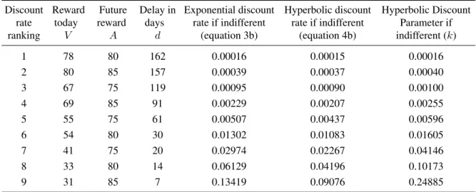
Table 1: Values of delay discounting task rewards and associated discount rates and parameters.

Discount rate ranking

Reward today

V

Future reward

A

Delay in days

d

Exponential discount rate if indifferent

(equation 3b)

Hyperbolic discount rate if indifferent

(equation 4b)

Hyperbolic Discount Parameter if indifferent (k)

1 78 80 162 0.00016 0.00015 0.00016

2 80 85 157 0.00039 0.00037 0.00040

3 67 75 119 0.00095 0.00090 0.00100

4 69 85 91 0.00229 0.00207 0.00255

5 55 75 61 0.00507 0.00437 0.00596

6 54 80 30 0.01302 0.01083 0.01605

7 41 75 20 0.02974 0.02267 0.04146

8 33 80 14 0.06129 0.04196 0.10173

9 31 85 7 0.13419 0.09076 0.24885

right side of Equation 6 or the reward on the left side of Equation 6, whenV,A, anddwere varied. Table 1 lists, for each trial, the smaller immediate reward (V), the larger later reward (A), the amount of the delay (d), the calculated exponential discount rate when the respondent is indifferent between the immediate and the future re-wards (as in Equation 3b), the calculated hyperbolic dis-count rate (as in Equation 4b), and the calculated hyper-bolic discount parameter (k). Although Table 1 tabulates the individual trials in increasing ranks of discount rates, the order of the presentation of the trials in the actual choice task was random with respect to the ranking of the discount rates, but the sequence was the same for all par-ticipants. The delays ranged from 1 week to 6 months and were presented as number of days from today.8 _An

exam-ple of one of the choices in this instrument was “Would you prefer R54 today or R80 in 30 days?” To prevent the participants from anchoring to one fixed larger later re-ward, the amountAalso varied by plus R5 to minus R5 from the larger later reward of R80. The exact numbers of days of delay and the possible smaller immediate re-wards were also varied. Although the combinations ofV,

d, andAwere varied for each of the delay discounting tri-als, they were designed to give 9 possible discount rates when the respondent became indifferent between the left and the right side of Equation 6.

The respondent’s SDR can be estimated from his choices in these trials. For instance, a respondent who prefers “R80 in 30 days” over “R54 today” (trial rank #6) can be inferred to have an exponential SDR of less than

8_{We did not include a front-end delay to the immediate reward,}

which has been used in some delay discounting tasks to control for transaction costs related to waiting that may confound pure time prefer-ence.

0.01302. If this same respondent also prefers “R55 to-day” over “R75 in 61 days” (trial rank #5), his SDR can be inferred to be greater than 0.00507. The combined information from these two trials suggests that this re-spondent’s actual SDR is bounded between 0.00507 and 0.01302. In this paper, following Kirby et al. (1999), we take the geometric mean between these two numbers as the SDR for this particular participant.9

A respondent who always chooses the larger later re-ward for each of the 9 trials can be inferred to have an SDR that is smaller than 0.00016 (but we do not know how much smaller); similarly, a respondent who always chooses the smaller sooner reward has an SDR that is greater than 0.13419 (but we do not know how much greater). For these respondents, we use the end point SDR, but in the regression analysis, we utilize Tobit re-gressions to take care of the left and right censoring in the data (explained further below).

Because we were unable to make a 100% guarantee of delivery of thefuturereward to our participants (due to logistical issues), we did not use real rewards in the delay discounting task.10

9_{Because the 9 trials were presented in random sequence and no}

titration was used to pinpoint an exact switching point from the smaller immediate reward to the larger later reward (or vice versa), some re-spondents gave answers that implied multiple discount rates. In these situations, we followed the same method as in Kirby et al. (1999, page 81), to calculate a single discount rate.

10_{It is not obvious from the literature whether having a real payoff}

(7)

2.2.2 Health measures

We used the SF12 health status instrument, which con-sisted of 12 questions that assessed symptoms, function-ing, and quality of life along two dimensions: mental and physical health (Ware et al., 1995). Examples of questions included in the SF12 are “Please tell me if your health now limits you in carrying out moderate ac-tivities that you might do during a typical day, such as walking to transport or helping at home? If so, how much?” and “How much of the time during the past 4 weeks did you have a lot of energy?” Also, one of the 12 questions was a self-assessed general health question in which the respondent was asked to rate his/her health into five categories, ranging from excellent to poor. Sep-arate scores for physical health (PCS12) and for mental health (MCS12) were obtained by weighting each ques-tion according to a formula (Ware et al., 1995). This in-strument has been validated in many developing countries in various languages including Zulu speaking populations in South Africa (available from QualityMetric.com) and was designed to be easily administered and answerable even by respondents who could not read.

2.2.3 Subjective probabilities of survival

The next set of questions asked individuals to rate their subjective probabilities of survival between 0% to 100% to measure how certain the respondent was that he/she would not die in the next 1, 5, or 10 years. A similar question was asked in the Health and Retirement Study (HRS) in the United States. A study by Smith et al. (2001) demonstrated that respondents not only could an-swer these questions, but also that their anan-swers indeed predicted their own mortality.

2.2.4 Planning and savings behavior

We asked questions about the respondents’ planning be-havior and savings bebe-havior. For the planning bebe-havior, we asked whether the respondents classified themselves as planning ahead all the time or living from day to day. Similarly, for savings behavior, we asked whether the respondents classified themselves as preferring to spend money to enjoy life today or to save more for the future. These questions were modeled after the US Panel Study of Income Dynamics. We also asked about the time hori-zon (ranging from a few months, a year, to the next sev-eral years) in the respondents’ planning and savings be-havior.

2.2.5 Expectations of economic and business situa-tion in the next two years

Because current versus future marginal utility of the hy-pothetical reward depends on the baseline income level in the two time periods, we asked all respondents whether they expected the economic situation of their community to improve a lot, improve a little, remain the same, de-cline a little, or dede-cline a lot in the next two years.

2.3 Data analysis

Because the main papers that studied the relationship be-tween age and SDR used different discount functions to calculate the SDR (Green et al., 1994 used a hyperbolic function but Read & Read, 2004, and Harrison et al., 2002, used exponential discount functions), we calcu-lated SDR using both the hyperbolic and the exponential discount functions (as depicted in Equations 3 and 4, re-spectively).

Using the calculated SDR for each participant, we ana-lyzed the bivariate relationships between the SDR and the respondents’ demographic characteristics, age, health, and expectations of subjective survival probability to live a certain number of years. We then performed a se-ries of multivariate regressions using the natural log of the SDR as the dependent variable, because the SDR is highly skewed without the log transformation. Given that the SDRs elicited by the hypothetical monetary tradeoffs are censored between 0.00016 and 0.13419, we used two-sided Tobit regressions to account for the left- and right-side censoring of the calculated SDR.11

To check the robustness of our results, we performed various regression diagnostics to flag potential outlier and

11_{The main advantage of using the two-sided Tobit was to account}

(8)

influential observations, compared results derived from regressions using both the full sample as well as the subsample after having deleted observations flagged by the regression diagnostics, examined results derived from OLS and Tobit regressions, and compared regression re-sults when the dependent variable was the (log of) the exponential SDR, the hyperbolic SDR, or the hyperbolic discount parameter (k). The main results and conclusions did not differ among these various alternative specifica-tions. Therefore, we present below the results obtained from two-sided Tobit regressions with ln(SDR) as the dependent variable, and briefly summarize the findings from these other alternative specifications.

Given that the delay discounting task used the number of days as the delay, all the discount rates are measured as discount rateper day.

3 Results

3.1 Descriptive statistics

Table 2 presents the mean and median SDRs for the full sample and for the subsamples defined by various so-ciodemographic variables. The first column also presents the mean and standard deviation for sociodemographic variables with a continuous distribution. The full sample consisted of 175 individuals, with 73% female and 46% married or cohabiting, and a mean age around 47 years, with a range from 18 to 91. Over 80% of the sample con-sisted of current or former small business owners. The respondents’ mean physical and mental health scores for the SF12 were 47.48 and 51.90, respectively, with stan-dard deviations of 12.1 and 10.9. The mean health scores in our population are similar to those in the United States (which have a normalized score of 50 and a standard de-viation of 10) (Ware et al., 1995). Twenty-five percent of respondents reported their health to be fair or poor (in-stead of excellent, very good, or good). In terms of the re-spondents’ expectations regarding their one-year survival probability, 38% (67 out of 175) said they were 100% confident that they would “live to this time next year,” and 21% stated at least a 60% chance of not living until the next year. The mean response was an 82% confidence of living to the next year. When we asked individuals their expectations to living to this time in five years (not shown in Table 2), 25% expressed a 100% confidence that they would live to this time in 5 years, and 31% of respondents expressed a 50–50 chance of living to the next 5 years. A similar pattern was found when we considered indi-viduals’ expectations to live 10 years. While 19% of re-spondents were 100% confident that they would be alive, 48% of respondents expressed a 50–50 percent chance or lower of being alive in 10 years.

The overall mean and median for the SDR (calculated using Equation 3b) for the full sample are 0.040 and 0.017 (per day).12 Because of the censoring of the SDRs due to the nature of the monetary delay discounting tasks used, (with a lower bound of 0.00016 and an upper bound of 0.134), there is also a significant number of individuals displaying the lowest SDR (7 in 175) and a large number of respondents displaying the highest SDR (24 in 175).

Table 2 also presents the mean and median SDRs grouped by sociodemographic variables and by health and survival expectations, and the Kruskal-Wallis test for significance in difference between groups. It is interest-ing to note that gender, marital status, business owner-ship, and income level of the respondent’s area of res-idence were not significantly related to SDR. Respon-dents with no education had significantly higher SDRs than those with some education.

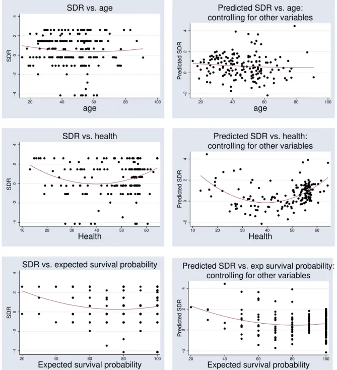
We next examined the bivariate relationship between the SDR and age, physical health, mental health, and sub-jective survival probability. Spearman rank correlation was insignificant between SDR and all of these variables (not shown in the table). This could either be because a relationship between these variables and the SDR does not exist, or the relationship is non-linear. Because the theoretical predictions (see Introduction above) suggest that the relationship between age and SDR may be non-linear and perhaps U-shaped, we next divided the sam-ple into approximate quintiles.13 It is interesting to note that older respondents do not have higher SDRs than the younger respondents. Figure 1 presents a plot of the raw and predicted values of SDR plotted against age, physical health, and expected survival probability, with and with-out controlling for other variables, respectively. Older people do not seem to have a higher discount rate than younger people, while health and survival expectations seem to have a U-shaped relationship with SDR.

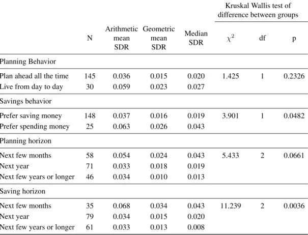
We also examined the relationship between SDRs and several behavioral variables that are often linked with time preference, such as willingness to plan for the fu-ture and to save money, and the results are shown in Ta-ble 3. We found that respondents who claimed that they had one year or longer planning or savings horizons had significantly lower SDRs than those with short horizons. Because planning and savings for long horizons require

12_{Kirby et al. (1999) and Kirby et al. (2002), using the same delay}

discounting tasks as ours, reportk-parameters (as thekin Equation 4a) instead of SDRs. Our sample shows a meank-parameter of 0.068 with a median of 0.023. These statistics are substantially higher than thek -parameters for both heroin addicts (mean of 0.025) and controls (mean of 0.013) studied by Kirby et al. (1999) in the U.S., but lower than the k-parameters (median of 0.12) found by Kirby et al. (2002) among the Tsimane’ Amerindians in Bolivia.

13_{Because of ties in the respondents’ age, health, or survival}

(9)

Table 2: Mean and median subjective discount rate (SDR), by sociodemographic variables (continued on next page).

Kruskal Wallis test of difference between groups

N

Arithmetic mean

SDR

Geometric mean SDR

Median

SDR χ

2

df p

Full Sample 175 0.040 0.017 0.020

Age (mean age = 46.52; s.d.=15.09)

Lowest Quintile 28 0.037 0.021 0.026 1.43 4 0.84 2nd Quintile 34 0.040 0.020 0.020

3rd Quintile 37 0.039 0.016 0.008 4th Quintile 40 0.041 0.012 0.019 Highest Quintile 36 0.044 0.018 0.019

Physical Health (mean = 47.48; s.d.=12.06)

Mental Health (mean = 51.90; s.d.=10.86)

1-Year Survival Probability (mean = 81.83; s.d.=19.71)

0 - 60% 36 0.063 0.028 0.043 16.77 3 0.00

70 - 80% 48 0.029 0.011 0.008

90% 24 0.018 0.010 0.008

100% 67 0.044 0.020 0.043

Overall business environment in 2 years

Improve a lot 10 0.029 0.014 0.020 2.86 4 0.58 Improve a little 52 0.040 0.020 0.043

The same 59 0.038 0.016 0.019

Decline a little 33 0.050 0.018 0.008 Decline a lot 10 0.024 0.008 0.008

Gender

Male 48 0.033 0.014 0.020 0.10 1 0.92

Female 127 0.043 0.018 0.019

a preference for waiting for a larger reward in the future, the results in Table 3 suggest that the level of “patience” as measured by SDR is consistent with the self-reported planning and savings behavior in our sample.14

14_{Because 16 significance tests were conducted for Tables 2 and 3,}

(10)

Table 2 (continued from last page). Mean and median subjective discount rate (SDR), by sociodemographic variables.

N

Arithmetic mean

SDR

Geometric mean

SDR

Median

SDR χ

2

df p

Marital Status

Married or Cohabiting 80 0.046 0.015 0.020 0.26 1 0.61 Single, divorced, widowed 95 0.036 0.018 0.019

Education Completed

None 11 0.090 0.062 0.134 11.92 5 0.04

Some primary 34 0.042 0.013 0.013

Primary completed 23 0.041 0.016 0.043

Some secondary 51 0.030 0.012 0.008

Secondary completed 37 0.037 0.019 0.020 Beyond secondary 19 0.041 0.020 0.020

Income

High Income 55 0.041 0.019 0.019 0.44 2 0.18

Middle Income 66 0.033 0.015 0.0187

Low Income 54 0.048 0.0164 0.040

Area dummies

Area N (high income) 25 0.033 0.012 0.008

Area A (high income) 30 0.048 0.027 0.031 8.07 5 0.15 Area J (middle income) 30 0.030 0.011 0.008

Area K (middle income) 36 0.036 0.020 0.043 Area C (low income) 26 0.058 0.025 0.043 Area G (low income) 28 0.038 0.011 0.008

Business Ownership

Business Owner or Past Owner 143 0.041 0.017 0.020 0.01 1 0.91

Never Owner 32 0.036 0.016 0.019

Know where to borrow R100

No 86 0.039 0.014 0.008 3.34 1 0.07

Yes 89 0.042 0.019 0.043

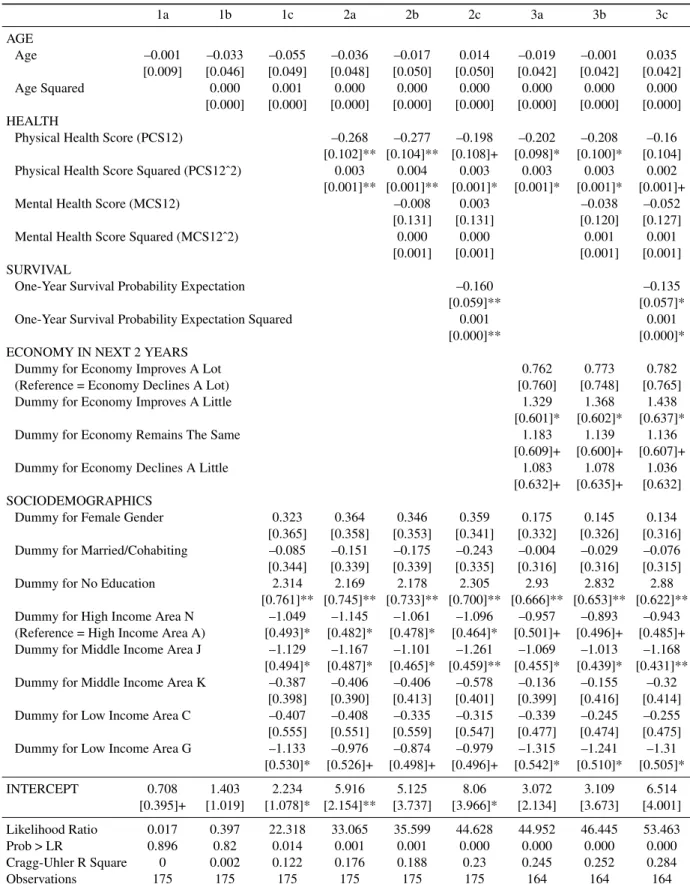
In addition to bivariate relationships, we next explored the relationship that SDR has with age, health, and sur-vival expectations, while controlling for other potential confounders. Using two-sided Tobit regression, we first regressed ln(SDR) on age and then also with age squared, but neither variable was significant (shown in Columns 1a and 1b of Table 4, respectively). We next included other demographic covariates plus area-specific dummy variables, and the results are shown in Column 1c. It is worth noting that Sozou and Seymour (2003) predicted a U-shaped relationship of the SDR and age, and empir-ical support for such a relationship was found by Read

differences between groups remains significant.

and Read (2004). However, in our study, this relation-ship was not statistically significant for either age alone or with both age and age squared jointly (test of joint sig-nificance,F(2, 144) = 0.34,p> 0.71). Gender and marital status were also insignificant, but those who had no edu-cation had a significantly higher SDR than those with at least some primary school education. Some of the area specific dummy variables were also significant.

(11)

Figure 1: Plot of raw and predicted subjective discount rate (SDR) as a function of age, health, and survival probability. Note that the vertical axis is ln(SDR·100).

with the SDR through its effect on mortality risk, we next added the one-year subjective probability of survival to the regression.15 Interestingly, as shown in specification 2c of Table 4, survival was not only highly significant, but

15_{Because the questions to elicit the SDRs were all framed with a}

delay that is less than one year, we use the 1-year survival probability in our analyses below; the results from using the 5- or 10-year survival probability variable are similar to those from the 1-year.

(12)

inclu-Table 3: Mean discount rate, by selected self-reported behavioral variables

N

Arithmetic mean SDR

Geometric mean

SDR

Median

SDR χ

2

df p

Planning Behavior

Plan ahead all the time 145 0.036 0.015 0.020 1.425 1 0.2326 Live from day to day 30 0.059 0.023 0.027

Savings behavior

Prefer saving money 148 0.037 0.016 0.019 3.901 1 0.0482 Prefer spending money 25 0.063 0.026 0.043

Planning horizon

Next few months 58 0.054 0.024 0.043 5.433 2 0.0661

Next year 71 0.033 0.018 0.019

Next few years or longer 46 0.034 0.010 0.013

Saving horizon

Next few months 35 0.068 0.034 0.043 11.239 2 0.0036

Next year 79 0.034 0.015 0.020

Next few years or longer 61 0.033 0.013 0.008

sion of the health variables. This suggests that the effect of survival on discounting is not via health, but part of the effect of health on discounting is via survival.

From specification (2c) in Table 4, it is apparent that the relationship between the SDR and both health and survival in our sample is U-shaped. This suggests that those in very poor health have high SDRs, but those in very good health also have high SDRs. Similarly, those with both high and low survival probabilities (but not those in between) display high SDRs. In fact, the nadir of the U-relationship between SDR and health occurred when PCS12 was 33, or less than one standard deviation below the mean physical health level of the sample. The nadir for the U-shaped relationship between the SDR and the one-year survival probability occurred at around 80%, or slightly below the mean subjective survival probability for the sample.

Because expanding income in the future may reduce the marginal utility of consumption in the future (and hence lead to greater discounting of the future), we next included a variable on the respondent’s subjective out-look for the overall economic environment in their com-munity in the next two years.16 _{(Eleven respondents did}

16_{Our survey unfortunately did not ask the respondents about their}

not answer this question and were excluded from subse-quent analysis.) This variable is only a crude proxy for the respondents’ subjective outlook for theirownfuture consumption opportunity, so the results should be inter-preted with caution. Columns 3a, 3b, and 3c show that those who thought the economy was going to worsen a lot in the next two years (the omitted dummy) had the low-est SDR. The U-shaped effect from survival probability on SDR continues to be significant. Under specification 3c, the linear term for physical health is no longer signifi-cant but the quadratic term remains signifisignifi-cant at the 10% level. The two variables are jointly significant (F(2,144) = 3.34, Prob > F = 0.0381), suggesting that physical health still bears a U-shaped relationship.

To control for any effect from business ownership (compared to never owning a business) and liquidity con-straints (which was crudely proxied for with a question that asked the respondent if he/she knew where to go if he/she needed to borrow 100 Rand), we included two dummy variables, which were found to be insignificant, while health and survival expectations continued to be significantly U-shaped with respect to SDR (not reported in Table 4). A likelihood-ratio test shows that the model

(13)

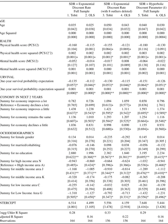
Table 4: Double sided Tobit regression, full sample (dependent variable = ln(SDR·100)).

1a 1b 1c 2a 2b 2c 3a 3b 3c

AGE

Age –0.001 –0.033 –0.055 –0.036 –0.017 0.014 –0.019 –0.001 0.035

[0.009] [0.046] [0.049] [0.048] [0.050] [0.050] [0.042] [0.042] [0.042]

Age Squared 0.000 0.001 0.000 0.000 0.000 0.000 0.000 0.000

[0.000] [0.000] [0.000] [0.000] [0.000] [0.000] [0.000] [0.000] HEALTH

Physical Health Score (PCS12) –0.268 –0.277 –0.198 –0.202 –0.208 –0.16 [0.102]** [0.104]** [0.108]+ [0.098]* [0.100]* [0.104] Physical Health Score Squared (PCS12ˆ2) 0.003 0.004 0.003 0.003 0.003 0.002

[0.001]** [0.001]** [0.001]* [0.001]* [0.001]* [0.001]+

Mental Health Score (MCS12) –0.008 0.003 –0.038 –0.052

[0.131] [0.131] [0.120] [0.127]

Mental Health Score Squared (MCS12ˆ2) 0.000 0.000 0.001 0.001

[0.001] [0.001] [0.001] [0.001] SURVIVAL

One-Year Survival Probability Expectation –0.160 –0.135

[0.059]** [0.057]*

One-Year Survival Probability Expectation Squared 0.001 0.001

[0.000]** [0.000]*

ECONOMY IN NEXT 2 YEARS

Dummy for Economy Improves A Lot 0.762 0.773 0.782

(Reference = Economy Declines A Lot) [0.760] [0.748] [0.765]

Dummy for Economy Improves A Little 1.329 1.368 1.438

[0.601]* [0.602]* [0.637]*

Dummy for Economy Remains The Same 1.183 1.139 1.136

[0.609]+ [0.600]+ [0.607]+

Dummy for Economy Declines A Little 1.083 1.078 1.036

[0.632]+ [0.635]+ [0.632] SOCIODEMOGRAPHICS

Dummy for Female Gender 0.323 0.364 0.346 0.359 0.175 0.145 0.134

[0.365] [0.358] [0.353] [0.341] [0.332] [0.326] [0.316] Dummy for Married/Cohabiting –0.085 –0.151 –0.175 –0.243 –0.004 –0.029 –0.076 [0.344] [0.339] [0.339] [0.335] [0.316] [0.316] [0.315]

Dummy for No Education 2.314 2.169 2.178 2.305 2.93 2.832 2.88

[0.761]** [0.745]** [0.733]** [0.700]** [0.666]** [0.653]** [0.622]** Dummy for High Income Area N –1.049 –1.145 –1.061 –1.096 –0.957 –0.893 –0.943 (Reference = High Income Area A) [0.493]* [0.482]* [0.478]* [0.464]* [0.501]+ [0.496]+ [0.485]+ Dummy for Middle Income Area J –1.129 –1.167 –1.101 –1.261 –1.069 –1.013 –1.168

[0.494]* [0.487]* [0.465]* [0.459]** [0.455]* [0.439]* [0.431]** Dummy for Middle Income Area K –0.387 –0.406 –0.406 –0.578 –0.136 –0.155 –0.32

[0.398] [0.390] [0.413] [0.401] [0.399] [0.416] [0.414] Dummy for Low Income Area C –0.407 –0.408 –0.335 –0.315 –0.339 –0.245 –0.255 [0.555] [0.551] [0.559] [0.547] [0.477] [0.474] [0.475] Dummy for Low Income Area G –1.133 –0.976 –0.874 –0.979 –1.315 –1.241 –1.31

[0.530]* [0.526]+ [0.498]+ [0.496]+ [0.542]* [0.510]* [0.505]*

INTERCEPT 0.708 1.403 2.234 5.916 5.125 8.06 3.072 3.109 6.514

[0.395]+ [1.019] [1.078]* [2.154]** [3.737] [3.966]* [2.134] [3.673] [4.001] Likelihood Ratio 0.017 0.397 22.318 33.065 35.599 44.628 44.952 46.445 53.463

Prob > LR 0.896 0.82 0.014 0.001 0.001 0.000 0.000 0.000 0.000

Cragg-Uhler R Square 0 0.002 0.122 0.176 0.188 0.23 0.245 0.252 0.284

Observations 175 175 175 175 175 175 164 164 164

(14)

that includes the dummy variables for business ownership and liquidity constraints is no better than the more parsi-monious model 3c, (likelihood ratio test chi-square (2 df) = 3.39, Prob > chi-square = 0.1838). We consider 3c to be the correct model for our analysis.

As a robustness check for our results, Table 5 presents regressions using different methods and using samples af-ter removal of observations flagged by regression diag-nostics. The first column of Table 5 is a repeat of specifi-cation 3c in Table 4, using double-sided Tobit and the full sample. The second column uses the same full sample but with ordinary least squares (OLS) as the regression method; the results are similar to those obtained from using Tobit. We next performed outlier diagnostics us-ing Studentized residuals and influence diagnostics usus-ing Cook’s D and DFITS (Belsley et al., 1980) to test whether our results are driven by specific observations. Interest-ingly, eight observations were flagged by all three diag-nostics. Removal of these problematic observations and then using Tobit (3rd_{column Table 5) or OLS (4}th_column

Table 5) showed that not only are our results still robust with these observations removed, but also our main vari-ables of interest (age, health, and survival) increased in statistical significance while remaining the same in mag-nitude. The similarity in the results derived from the To-bit and the OLS estimations suggests that any inconsis-tency in coefficient estimates due to violations of Tobit assumptions (heteroscedasticity and non-normality of er-rors) does not bias the Tobit estimates beyond the incon-sistent estimates from OLS.17Columns 5 and 6 of Table 5 present the Tobit and OLS regressions results using the full sample but using ln(k·100) as the dependent variable.

The results are very similar to those with the exponential form ln(SDR·100) as the dependent variable.

Finally, both the adjusted R-square in the OLS model and the Cragg-Uhler R-square in the Tobit model are be-tween 0.16 and 0.33, which is comparable to the adjusted R-squares in the OLS models by Read and Read (2004) that range from 0.04 to 0.24, depending on the time hori-zon used in the discounting task.

4 Discussion

Several of our findings are new. Our first main finding is that age is not a significant predictor of time preference, which is in contrast to the findings in Green et al. (1994)

17_{OLS estimates are inconsistent with censored data. Tobit estimates,}

which take care of the data censoring issue, are also inconsistent when the residual errors are non-normal or heteroscedastic. The normality as-sumption was violated in the full sample Tobit (n = 164, Wilks-Shapiro Test W = 0.978, p < 0.05) but not in the subsample Tobit (Table 5 col-umn 3) (n = 156, Wilks-Shapiro Test W = .985, p > 0.05). The assump-tion of homoscedasticity cannot be rejected for both the full and the subsample, using the White test (p > 0.45).

and Read and Read (2004). Our findings may differ from those of these authors for at least two reasons. One is that only 25% of our sample consists of people over the age of 55 and that our sample may not contain enough older peo-ple to show an age effect, whereas Read and Read (2004) concentrated their sample selection based on three age strata, with the oldest strata around age 70. Notably, we are comparing different kinds of people in very different environments. The other reason is that health and espe-cially survival probability, not age, may be a true underly-ing determinant of people’s SDRs. In populations where age does correlate well with health and survival proba-bility, the effect of these other variables on SDRs can be well-manifested by the effects of age. However, be-cause be-causes of morbidity and mortality in South Africa are not necessarily related to age, age is no longer a strong predictor of health and expected survival and, hence, of SDRs.

Our second main finding is the U-shaped relationship between physical health and the SDR. Although the re-lationship is attenuated both in magnitude and in signifi-cance with the inclusion of survival probability, the linear and the quadratic terms for physical health remainjointly significantat the 5 percent significance level for all spec-ifications. The few studies that did examine the relation-ship between health and the SDR did not find evidence of such a relationship probably because of the crude health measures used and because of the lack of a non-linear term in these other studies’ regressions. Respondents in our sample with average health have a lower discount rate than those who are very healthy or very sick, and this could be due to several reasons. We note that we find a higher SDR among people with very poor health, while simultaneously controlling for expected survival probability (and hence “wanting to deplete resources be-fore death” cannot completely explain this finding). Ac-cording to Trostel and Taylor (2001), Olsho (2006), and Finkelstein et al. (2008), the ability to enjoy consumption depends on an individual’s health, and the healthier an individual, the greater the marginal utility of consump-tion. Because health generally declines over the life cy-cle, individuals should have a high SDR when healthy and, thus, enjoy consumption while they still can. Al-ternatively, people with very poor health may have more immediate need for cash to pay for medical care or for daily survival (perhaps because they are too sick to work), hence the unwillingness to wait for the larger reward. Un-fortunately, our data set limits us from testing these expla-nations, which must await future studies.

(15)

Table 5: Double-sided Tobit and OLS regressions, by sample (dependent variable = ln(SDR·100)).

SDR = Exponential SDR = Exponential SDR = Hyperbolic Discount Rate Discount Rate Discount Parameter (k)

Full Sample (with 8 outliers deleted) Full Sample 1. Tobit 2. OLS 3. Tobit 4. OLS 5. Tobit 6. OLS AGE

Age 0.035 0.025 0.050 0.043 0.040 0.030

[0.042] [0.038] [0.034] [0.032] [0.047] [0.042]

Age Squared 0.000 0.000 0.000 0.000 0.000 0.000

[0.000] [0.000] [0.000] [0.000] [0.000] [0.0004] HEALTH

Physical health score (PCS12) –0.160 –0.115 –0.155 –0.121 –0.180 –0.130

[0.104] [0.081] [0.084]+ [0.069]+ [0.116] [ 0.091] Physical health score squared (PCS12ˆ2) 0.002 0.002 0.002 0.002 0.003 0.002

[0.001]+ [0.001]+ [0.001]* [0.001]* [0.001]+ [0.001]+

Mental health score (MCS12) –0.052 –0.014 –0.017 0.008 –0.064 –0.022

[0.127] [0.107] [0.101] [0.089] [0.138] [0.116] Mental health score squared (MCS12ˆ2) 0.001 0.000 0.000 0.000 0.001 0.000

[0.001] [0.001] [0.001] [0.001] [0.002] [0.001] SURVIVAL

One-year survival probability expectation –0.135 –0.112 –0.130 –0.115 –0.151 –0.126 [0.057]* [0.046]* [0.053]* [0.046]* [0.064]* [0.051]* One-year survival probability expectation squared 0.001 0.001 0.001 0.001 0.001 0.001

[0.000]* [0.000]* [0.000]** [0.000]** [0.000]* [0.000]* ECONOMY IN NEXT 2 YEARS

Dummy for economy improves a lot 0.782 0.726 1.094 1.059 0.858 0.796

(Reference = Economy declines a lot) [0.765] [0.699] [0.613]+ [0.577]+ [0.836] [.761]

Dummy for economy improves a little 1.438 1.238 1.421 1.311 1.593 1.374

[0.637]* [0.543]* [0.595]* [0.542]* [0.695]* [ 0.589]*

Dummy for economy remains the same 1.136 1.010 1.293 1.207 1.254 1.116

[0.607]+ [0.503]* [0.584]* [0.525]* [0.664]+ [0.548]*

Dummy for economy declines a little 1.036 0.831 0.998 0.890 1.155 0.931

[0.632] [0.512] [0.600]+ [0.530]+ [0.694]+ [0.560]+ SOCIODEMOGRAPHICS

Dummy for female gender 0.134 0.014 –0.235 –0.292 0.145 0.014

[0.316] [0.278] [0.221] [0.204] [0.347] [0.305 ]

Dummy for married/cohabiting –0.076 –0.146 0.098 0.038 –0.056 –0.132

[0.315] [0.270] [0.252] [0.227] [0.349] [0.299]

Dummy for no education 2.880 1.996 2.382 1.840 3.195 2.234

[0.622]** [0.368]** [0.567]** [0.381]** [0.695]** [0.415]**

Dummy for high income area N –0.943 –0.860 –0.664 –0.624 –1.032 –0.941

(Reference = High income area A) [0.485]+ [0.424]* [0.396]+ [0.366]+ [0.536]+ [0.468]*

Dummy for middle income area J –1.168 –1.005 –0.910 –0.814 –1.289 –1.112

[0.431]** [0.371]** [0.344]** [0.312]* [0.476]** [0.410]**

Dummy for middle income area K –0.320 –0.174 –0.175 –0.082 –0.365 –0.208

[0.414] [0.356] [0.338] [0.303] [0.461] [0.396]

Dummy for low income area C –0.255 –0.142 –0.032 0.025 –0.261 –0.139

[0.475] [0.394] [0.408] [0.363] [0.529] [0.440]

Dummy for Low Income Area G –1.310 –1.127 –0.792 –0.713 –1.432 –1.231

[0.505]* [0.450]* [0.347]* [0.331]* [0.556]* [0.496]*

INTERCEPT 6.514 4.499 5.556 4.159 7.648 5.444

[4.001] [3.105] [3.478] [2.918] [4.416]+ [3.428]

Cragg-Uhler R Square 0.28 0.33 0.29

Adjusted R Square 0.16 0.22 0.16

Observations 164 164 156 156 164 164

(16)

!" #!!" $%!!!" $%#!!" &%!!!" &%#!!" '%!!!" '%#!!" (%!!!" (%#!!"

$#)$*" &!)&(" &#)&*" '!)'(" '#)'*" (!)((" (#)(*" #!)#(" ##)#*" +!)+("

,-./" 01&!!("

2/3-./" 01&!!("

456-." 01&!!("

,-./" 70&!!#"

2/3-./" 70&!!#"

456-." 70&!!#"

!" #!!" $%!!!" $%#!!" &%!!!" &%#!!" '%!!!" '%#!!" (%!!!" (%#!!"

$#)$*" &!)&(" &#)&*" '!)'(" '#)'*" (!)((" (#)(*" #!)#(" ##)#*" +!)+("

,-./" 01&!!("

2/3-./" 01&!!("

456-." 01&!!("

,-./" 01$**8"

2/3-./" 01$**8"

456-." 01$**8"

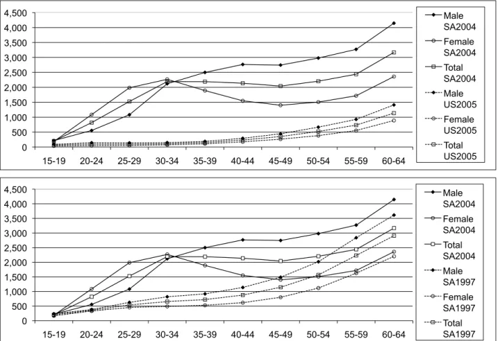
Figure 2: Comparison of age-specific death rates per 100,000: S.A. 2004 vs. U.S. 2005 and S.A. 2004 vs. S.A. 1997. (Source: Statistics South Africa, 2006, and Kung et al., 2008.)

never come. It is somewhat perplexing as to why those with a very high expected survival probability also highly discount the future; an explanation for this finding must also await future studies.

In spite of our inability to dig deeper into the many mechanisms by which health and survival probability should have U-shaped relationships with SDR, the po-tential importance of health and survival probability as determinants of delay discounting is a novel finding. The inclusion of comprehensive measures of health status and expected survival probability is an important contribu-tion. The inclusion of these variables is already implicit in the theories that we reviewed, but we think it is impor-tant to include these variables more explicitly in empiri-cal specifications in order to tease apart the contributions of each of these variables and to understand the true fac-tors that determine the SDR. From the empirical stand-point, the use of the SF12 instrument as a comprehen-sive measures of health status is less subject to system-atic measurement error than single question health sta-tus measures (Dow et al., 1997) and may be what

(17)

monotonically increased with age. This is especially evi-dent among females of child-bearing age in South Africa, who have higher HIV prevalence and AIDS deaths than males (Shisana et al., 2005).18

4.1 Limitations

The study is subject to several limitations and the results must be interpreted with caution. The first limitation is that we had a small sample that consisted of mostly busi-ness operators. While this gave us confidence that the answers to questions involving monetary tradeoffs were less likely to be subject to the problems of low mathe-matical literacy, it is unclear whether our results from a mostly mathematically-literate population are generaliz-able to other populations in the developing world. Nev-ertheless, as shown in Table 2 and in regressions that in-cluded business ownership as a dummy variable (not re-ported in the tables), business owners did not have signif-icantly different SDRs than non-owners.

The second limitation is that we did not have good measures of household assets and income; we only have measures of the income strata where the respondents resided. Relative to the highest income area, the fixed ef-fects for low and middle income areas were consistently negative and some statistically significant and negative, which indicates that respondents in the lower income ar-eas have lower SDRs than those from the highest income area. This finding is opposite to that found by Green et al. (1996), who found that income, not age, was associ-ated with SDR, and that found by Read and Read (2004), who also included income strata for their time prefer-ence study among populations of the United Kingdom and found that high income strata were associated with a lower SDR. This seeming contradiction may be because all of our respondents are poor, just that some are less poor than others. Even our “high income” strata would be considered below the lowest income strata in the study populations of these other authors.

4.2 Study implications

The relationship between individual characteristics and delay discounting is an important area for future research. Given the robust relationship that survival probability has with the SDR and the marginally significant relationship between health and the SDR, there may be a role for the inclusion of health and survival probability into delay dis-counting models and empirical studies. The possibility

18_{The age-specific mortality per 100,000 in the U.S. (which is}

simi-lar to that in Denmark and the U.K.) is monotonically increasing with respect to age, and has remained stable for many decades. The pattern is similar to that found in South Africa for 1997, except with a much lower mortality rate per 100,000 for each age-bracket.

of non-linear relationships that the SDR has with age, health, and survival probability should also be taken into consideration in future empirical specifications.

References

Ainslie, G. (1975). Specious reward: A behavioral theory of impulsiveness and impulse control. Psychological Bulletin,82, 463–496.

Becker, G. S., & Mulligan, C. B. (1997). The endogenous determination of time preference.Quarterly Journal of Economics, 112, 729–758.

Belsley, D. A., Kuh, E., & Welsch, R. E. (1980). Re-gression Diagnostics: Identifying Influential Data and Sources of Collinearity. New York: John Wiley & Sons.

Bickel, W. K., Odum, A. L., & Madden G. J. (1999). Im-pulsivity and cigarette smoking: Delay discounting in current, never, and ex-smokers.Psychopharmacology,

146, 447–454.

Boettiger, C. A., Mitchel, J. M., Tavares, V. C., Robert-son, M., Joslyn, G., D’Esposito, M., & Fields, H. L. (2007). Immediate reward bias in humans: Fronto-parietal networks and a role for the catechol-O -methytransferase 158Val/Valgenotype. Journal of Neu-roscience, 27, 14383–14391.

Börsch-Supan, A., & Stahl, K. (1991). Life cycle savings and consumption constraints. Journal of Population Economics,4, 233–255.

Chao, L. W., Pauly, M. V., Szrek, H., Sousa Pereira, N., Bundred, F., Cross, C., & Gow, J. (2007). Poor health kills small business: Illness and microenterprises in South Africa.Health Affairs, 26, 474–482.

Chapman, G. B., Brewer, N.T., Coups, E.J., Brownlee, S., Leventhal, H., & Leventhal, E. A. (2001). Value for the future and preventive health behavior. Journal of Experimental Psychology: Applied,7, 235–250. Chapman, G. B., & Coups, E.J. (1999). Time preferences

and preventive health behavior: Acceptance of the In-fluenza Vaccine. Medical Decision Making,19, 307– 314.

Chapman, G.B. (2005). Short-term cost for long-term benefit: Time preference and cancer control. Health Psychology,24, S41-S48.

Coller, M., & Williams, M. B. (1999). Eliciting individ-ual discount rates. Experimental Economics,2, 107– 127.

Dow, W., Gertler, P., Schoeni, R. F., Strauss, J., & Thomas, D. (1997). Health care prices, health and la-bor outcomes: Experimental evidence. RAND Lala-bor and Population Program Working Paper 97–01. Finkelstein, A., Luttmer, E. F. P., & Notowidigdo, M. J.

(18)

ef-fect of health on the marginal utility of consumption. Harvard Kennedy School Faculty Research Working Papers Series RWP08–036, June 2008.

Frederick, S., Loewenstein, G., & O’Donoghue, T. (2002). Time discounting and time preference: A crit-ical review. Journal of Economic Literature,40, 351– 401.

Glimcher, P. W, Kable, J. W., & Louie, K. (2007). Neu-roeconomic studies of impulsivity: Now or just as soon as possible? American Economic Review, 97, 142– 147.

Green, L., Fry, A. F., & Myerson, J. (1994). Discounting of delayed rewards: A life-span comparison. Psycho-logical Science, 5(1), 33–36.

Green, L., Myerson, J., Lichtman, D., Rosen, S., & Fry, A. (1996). Temporal discounting in choice between delayed rewards: The role of age and income. Psy-chology and Aging,11,79–84.

Halevy, Y. (2005). Diminishing impatience: Disentangling time preference from uncer-tain lifetime. University of British Columbia Department of Economics Working Paper. http://papers.ssrn.com/sol3/papers.cfm?

abstract_id=612476 accessed on April 15, 2008). Harrison, G. W., Lau, M. I., & Williams, M. B. (2002).

Estimating individual discount rates in Denmark: A field experiment.The American Economic Review,92, 1606–1617.

Jevons, H. S. (1905). Essays on Economics. London: MacMillan.

Jevons, W. S. (1888). The Theory of Political Economy. London: MacMillan.

Johnson, M. W., & Bickel, W. K. (2002). Within-subject comparison of real and hypothetical money rewards in delay discounting.Journal of the Experimental Analy-sis of Behavior, 77, 129–146.

Kable, J. W., & Glimcher, P. W. (2007). The neural cor-relates of subjective value during intertemporal choice.

Nature Neuroscience,10, 1625–1633.

Kirby, K. N. (1997). Bidding on the future: Evi-dence against normative discounting of delayed re-wards.Journal of Experimental Psychology: General,

126, 54–70.

Kirby, K. N., Godoy, R., Reyes-Garcia, V., Byron, E., Apaza, L., Leonard, W., Perez, E., Vadez, V., & Wilkie, D. (2002). Correlates of delay-discount rates: Evi-dence from Tsimane’ Amerindians of the Bolivian rain forest.Journal of Economic Psychology, 23, 291–316. Kirby, K. N., & Marakovic, N. N. (1995). Model-ing myopic decisions: Evidence for hyperbolic delay-discounting within subjects and amounts. Organiza-tional Behavior and Human Decision Processes, 64, 22–30.

Kirby, K. N., Petry, N. M., & Bickel, W. K. (1999). Heroin addicts have higher discount rates for delayed rewards than non-drug-using controls. Journal of Ex-perimental Psychology: General, 128, 78–87.

Kirby, K. N., Winston, G. C., & Santiesteban, M. (2005). Impatience and grades: Delay-discount rates correlate negatively with college GPA.Learning and Individual Differences,15, 213–222.

Kung, H. C., Hoyert, D. L., Xu, J. Q., and Murphy, S. L. (2008). Deaths: Final data for 2005. National Vi-tal Statistics Reports; Vol 56 no 10. Hyattsville, MD: National Center for Health Statistics.

Loewenstein, G., & Prelec, D. (1992). Anomalies in intertemporal choice: Evidence and an interpretation.

The Quarterly Journal of Economics,107,573–597. Long, J. S. (1997). Regression Models for Categorical

and Limited Dependent Variables. Thousand Oaks: Sage Publications.

Madden, G. J., Begotka, A. M., Raiff, B. R., & Kastern, L. L. (2003). Delay discounting of real and hypothet-ical rewards. Experimental and Clinical Psychophar-macology,11,139–145.

McClure, S. M., Ericson, K. M., Laibson, D. I., Loewen-stein, G., & Cohen, J. D. (2007). Time discounting for primary rewards. The Journal of Neuroscience, 27), 5796–5804.

McClure, S. M., Laibson, D. I., Loewenstein, G., & Co-hen, J. D. (2004). Separate neural systems value im-mediate and delayed monetary rewards. Science,306, 503–507.

Olsho, L. (2006). Spend it while you can still enjoy it: Health, longevity, aging, and consumption in the life cycle. Department of Economics Working Paper, Uni-versity of Wisconsin-Madison. August 2006.

Pender, J. L. (1996). Discount rates and credit markets: Theory and evidence from rural India.Journal of De-velopment Economics,50, 257–296.

Rachlin, H. (1989). Judgment, Decision, and Choice.

New York: Freeman.

Rae, J. (1834).The Sociological Theory of Capital. Lon-don: MacMillan.

Read, D. (2003). Intertemporal choice. London School of Economics and Political Science Working Paper LSEOR 03.58. http://www.lse.ac.uk/collections/ operationalResearch/pdf/working%20paper%2003– 581.pdf accessed on April 15, 2008.

Read, D., & Powell, M. (2002). Reasons for sequence preferences. Journal of Behavioral Decision Making,

15, 433–460.

Read, D., & Read, N. L. (2004). Time discounting over the lifespan.Organizational Behavior and Human De-cision Processes,94, 22–32.

(19)

461–481.

Shisana, O., Rehle, T., Simbayi, L. C., Parker, W., Zuma, K., Bhana, A., et al. (2005). South African National HIV Prevalence, HIV Incidence, Be-haviour and Communication Survey, 2005. South African Human Sciences Research Council (HSRC) (http://www.hsrcpress.co.za/index.asp?id=2134 ac-cessed on 25 January 2006)

Shoda, Y., Mischel, W., & Peake, P. K. (1990). Predicting adolescent cognitive and self-regulatory competencies from preschool delay of gratification: Identifying di-agnostic conditions. Developmental Psychology, 26, 978–986.

Smith, V. K., Taylor, D. H. Jr., & Sloan, F. A. (2001). Longevity expectations and death: Can people predict their own demise? American Economic Review, 91, 1126–1134.

Sozou, P. D., & Seymour, R. M. (2003). Augmented discounting: Interaction between ageing and time-preference behaviour. Proceedings of the Royal Soci-ety of London Series B,270, 1047–1053.

Statistics South Africa. 2006. Adult Mortality (Age 15– 64) Based on Death Notification Data in South Africa: 1997–2004. Report No. 08–09–05 (2006).

Trostel, P. A., & Taylor, G. A. (2001). A theory of time preference.Economic Inquiry, 39, 379–395.

Ware, J. E., Kosinski, M., & Keller, S. D. (1995).How to Score the SF-12 Physical and Mental Health Summary Scale, 2d ed. Boston: Health Institute, New England Medical Center.