www.ann-geophys.net/32/449/2014/ doi:10.5194/angeo-32-449-2014
© Author(s) 2014. CC Attribution 3.0 License.
Annales
Geophysicae
Excitation of planetary electromagnetic waves in the inhomogeneous
ionosphere
Yu. Rapoport1, Yu. Selivanov2, V. Ivchenko1, V. Grimalsky3, E. Tkachenko1, A. Rozhnoi4, and V. Fedun5
1Kyiv National Taras Shevchenko University, 2, Glushkova Av., Build. 1, 03680 Kyiv, Ukraine 2Space Research Institute NASU-NSAU, 40, Glushkov Av., 03680, Kiev 187, Ukraine 3University of Morelos, Av. Universidad, 1001, Z.P. 62210, Cuernavaca, Morelos, Mexico
4Institute of Physics of the Earth, Russian Academy of Sciences, 10 B. Gruzinskaya, Moscow, 123995, Russia
5Space Systems Laboratory, Department of Automatic Control and Systems Engineering, University of Sheffield, Sheffield, S1 3JD, UK
Correspondence to:V. Fedun ([email protected])
Received: 25 March 2013 – Revised: 15 January 2014 – Accepted: 6 February 2014 – Published: 25 April 2014
Abstract. In this paper we develop a new method for the analysis of excitation and propagation of planetary electro-magnetic waves (PEMW) in the ionosphere of the Earth. The nonlinear system of equations for PEMW, valid for any height, from D to F regions, including intermediate altitudes between D and E and between E and F regions, is derived. In particular, we have found the system of nonlinear one-fluid MHD equations in theβ-plane approximation valid for the ionospheric F region (Aburjania et al., 2003a, 2005). The se-ries expansion in a “small” (relative to the local geomagnetic field) non-stationary magnetic field has been applied only at the last step of the derivation of the equations. The small mechanical vertical displacement of the media is taken into account. We have shown that obtained equations can be re-duced to the well-known system with Larichev–Reznik vor-tex solution in the equatorial region (see e.g. Aburjania et al., 2002). The excitation of planetary electromagnetic waves by different initial perturbations has been investigated numeri-cally. Some means for the PEMW detection and data pro-cessing are discussed.
Keywords. Ionosphere (modeling and forecasting)
1 Introduction and formulation of the problem
In recent years a considerable effort has been made for treating waves propagation problems in the inhomogeneous Earth’s ionosphere (see e.g. Clark et al., 1971; Rapoport et al., 2004, 2009; Sorokin and Fedorovich, 1982; Alperovich
imposed by magnetospheric sources, for instance, by the flux transfer events (FTE). Therefore, they are important for un-derstanding the coupling mechanisms between the magneto-sphere and ionomagneto-sphere.
The purpose of the present study is to develop the gen-eral theory of excitation of nonlinear PEMWs in the iono-sphere of the Earth. Previous studies of PEMW (see e.g. Khantadze, 1973; Aburjania et al., 2003a; Kaladze et al., 2003; Aburjania and Chargazia, 2011) were limited by as-suming that the relationships between the components of the conductivity tensor σ⌢characterises only strongly pro-nounced D, E or F regions with “purely” isotropic, gyrotropic and non-gyrotropic but anisotropic⌢σ, respectively (see e.g. Guglielmi and Pokhotelov, 1996). By taking into account such assumptions, analytical solutions of the system of equa-tion for PEMW in the form of vortexes or solitons were de-rived (see e.g. Aburjania et al., 2002). However, to under-stand the effects of non-stationarity and inhomogeneities in the nonlinear dissipative ionosphere, more general methods are necessary. Additionally, this approach is important for systematic detection of PEMW by joint satellite and ground-based observations campaigns.
The paper has the following structure. The formulation of the problem and initial equations for PEMWs are outlined in Sect. 1. In Sect. 2 we build the nonlinear system of equations for PEMW. The nonlinear equations for PEMW at arbitrary heights from D to F regions in the “linear Ohm’s law” ap-proximation outlined in Sect. 3. The applications to the “po-lar” and “equatorial” regions are outlined in Sect. 4. In Sect. 5 we implement an algorithm with accounting for the non-linearity in the ionospheric current (nonlinear Ohm’s law) for the F region of the ionosphere. In Sect. 6, based on the spectral-grid approximation (see Arakawa, 1997) the non-linear PEMW, vortex and soliton structures have been anal-ysed numerically. Different scenarios of PEMW excitation for various geophysical conditions at the near-pole region in the approximation of the “linear Ohm’s law” are presented. Section 7 is the discussion and conclusion.
2 Formulation of the problem.
Equations for PEMWs in the magnetosphere– ionosphere–atmosphere–lithosphere (MIAL) system
Let us consider the ionosphere as a spherical layer around the Earth (see Fig. 1). Based onβ-plane approximation, fluid incompressibility and by neglecting gravity, the system of MHD equations, for the motions in theβ-plane, can be writ-ten as (Landau et al., 2004; Sorokin and Fedorovich, 1982; Guglielmi and Pokhotelov, 1996; Kaladze et al., 2003)
∂U
∂t +(U∇)U= FA
ρ0 +
2 [U×0]−∇P ρ0 −
γU; (1)
curlE= −c−1 ∂H
∂t
; curlH =4π c−1j; (2)
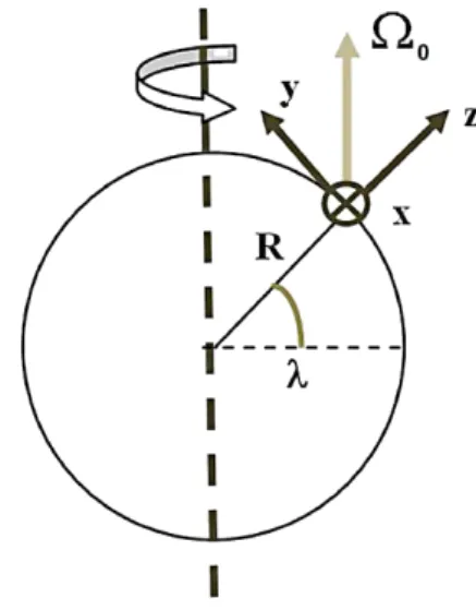
Fig. 1.Coordinate system of the model.Xaxis pierces the plane of figure.Ris the radius of the Earth,0is the angular velocity of the Earth rotation;λ=0 andλ=π/2 correspond to equator and pole, respectively.
divH =0; divU=0; (3)
j =σ||E˜||+σPE˜⊥+σHhh× ˜Ei. (4)
Here c is the speed of light; U, ρ0 are the velocity and density of media at heightzof the chosenβ-plane, respec-tively;0is the rotation parameter; γ is the effective
me-chanical damping parameter;E,H are the electric and
mag-netic fields; E˜ =E+c−1[U×H] is the electric field in
the moving media;j is the electric current density;FA= c−1
j×H
is the Ampere force.
parameters due to vertical displacement is negligibly small, not to violate the condition of incompressibility for the per-turbations. Respectively, the relation of “zero divergence” is valid and the corresponding presentation of the velocityX, Y components through ONE functionξ (see Eq. 12) are ap-plicable for the horizontal components of velocity, even if a small vertical component corresponding to relatively small vertical displacement is also included in our model. There-fore, our model is internally consistent. The errors made by assuming that the magnetic and rotation axes coincide is of the same order as the errors inherent in theβ-plane approxi-mation (see e.g. Aburjania et al., 2005; Kaladze et al., 2003). For the above scales of disturbances, the consequences of the misalignment of both axes, which is about 0.2 rad, are be-yond the accuracy of theβ-plane approximation and, there-fore, cannot change the results qualitatively. Note that the variation of ion mass, reflecting the changing in composition, is included into the model through the elements of conduc-tivity tensor in the Eq. (4).
Before introducing the terms of conductivity tensor in the Eq. (4), let us specify the magnetic field. We define the ve-locityUand total magnetic fieldHby the relations:
U=U0+U′; H =H0+H′; h≡H/H;
h0≡H0/H0; h′≡H′/H0. (5)
HereU0andH0are the stationary velocity and geomagnetic
field;U′ andH′ are the small perturbations of the velocity and magnetic field;h,h0are the unit vectors that determine
the directions of the total and stationary geomagnetic field; H0 andH=
q
(H0+H′)2
are the values of stationary ge-omagnetic and total magnetic field;h′determines the
direc-tion of the non-stadirec-tionary part of the magnetic field. We also assume that√h′2≪1. By taking into account the geometry of the model (see Fig. 1), dipole approximation of the ge-omagnetic field, and Eq. (3), the stationary (wind) velocity and magnetic field can be written as follows:
U0= U0x(y), U0y(x),0
; H0= 0, H0y(y, z), H0z(y, z); H0=
q
H0y2 +H0z2; (6)
h0=(0, h0y, h0z); h0y,z≡H0y,z H0
.
Herex,yandzare directed along the parallel, meridian and vertical, respectively; λ=0 and λ=π/2 are the latitudes which correspond to the equator and pole, respectively (see Fig. 1). In approximation z/R≪1 the components of the stationary geomagnetic fieldH0y andH0z, and the rotation parameter0can be represented as (see e.g. Kaladze et al.,
2003) H0y≈Heq
1−2z
R
cosλ; H0z≈ −2Heq
1− z
2R
sinλ;
Heq=H0y(λ=0, z=0);
0= 0, 0y, 0z
=0(0,cosλ,sinλ) . (7) Note that the chosen coordinate dependence of the sta-tionary velocity in Eqs. (6) also satisfy the second equation in Eqs. (3). Therefore, as it follows from the relations for the stationary geomagnetic field Eqs. (7), with accuracy to z/R≪1, we obtain (Kaladze et al., 2003)
∂H0z ∂z +
∂H0y ∂y =0; ∂H0z
∂y = ∂H0y
∂z ; ∂
∂y = 1 R
∂
∂λ. (8)
The elements of conductivity tensor are defined by the well-known formulas (see e.g. Guglielmi and Pokhotelov, 1996; Sorokin and Fedorovich, 1982; Kaladze et al., 2003):
σ||=en H
ω Hi νi +
ωHe νe
;
σP= en H
ωHeνe
ω2He+ν2 e
+ ωHiνi ω2Hi+νi2
! ;
σH= eh H
ω2He
ω2He+ν2 e
− ω
2 Hi ωH2i+νi2
!
. (9)
Here σ||, σP, σH are the parallel, Pedersen, and Hall con-ductivities, respectively;ωHe,iare the electron and ion gyro-frequencies (defined by the value of the total magnetic field H);νe is the sum of collision frequencies of electrons with neutrals and ions;νi is the collision frequency of ions with neutrals. Considering Eq. (4) as algebraic equation for elec-tric fieldE and by taking into account the second equation
in Eqs. (2), the electric field in the moving mediaE˜ can be
expressed in terms of the magnetic fieldH as ˜
E= c
4π σeff{
curlH−q1[h×curlH]+q2(h·curlH)h} (10)
and, therefore, we can exclude the electric field from the sys-tem of MHD equations for PEMW. Here
σeff=
σP2+σH2 σP ;
q1= σH σP;
q2= σeff
σ|| −1.
The coefficients q1 and q2 correspond to the “transverse” electric field (defined by the Hall current) and to the “lon-gitudinal” electric field, respectively.
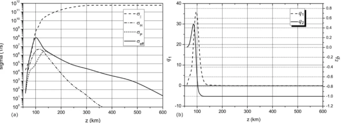
Fig. 2.The dependence of ionosphere conductivitiesσ0,σH,σPandσeffas a function of height,z, are shown in(a). The values of coefficients
q1,2vs. height,z, are plotted at(b).q1andq2are coefficients in the expressions, corresponding to the “transverse” electric field, determined by Hall current and “longitudinal” electric field (see Eq. 10).
anisotropic and non-gyrotropic (Fig. 2a). The present model is also applicable for intermediate heights (i.e. for the heights between D and E, and between E and F regions), where the relationships mentioned above betweenq1andq2are not sat-isfied (see also Fig. 2b). The elements of conductivity tensor (see Eq. 9) depend on total magnetic field H (see Eq. 8) which is the function of the non-stationary magnetic field H′ (see Eq. 5). Therefore, the electric current Eq. (4) and electric field Eq. (10) become nonlinear. Due to such non-linearity, hereafter we will call Eq. (4) as “nonlinear Ohm’s law”. In the linear limit (i.e. in Eq. (4)) h is replaced by
h0 and the elements of the conductivity tensor(σ )⌢ are re-placed by corresponding linear values, the Eq. (4) become linear. In this case, hereafter, we will call Eq. (4) as “lin-ear Ohm’s law”. Practically, it corresponds to replacement ofH byH0 in Eqs. (9) in all dependent on magnetic field terms. Theβ-plane approximation require implementation of “the method of frozen coefficients” (see e.g. Aburjania et al., 2003a; Kaladze et al., 2003) and satisfying of the following assumptions
∂H′ ∂z =0;
∂U′
∂z =0; ∇ρ=0. (11)
Second and third relations in Eq. (11) correspond to the case of neglecting gravity stratification. However, by taking into account equations for the stationary geomagnetic field, that is, Eqs. (7) and (8), we should require∂H0y,z/∂z6=0 and, therefore,∂h0/∂z6=0,∂h′/∂z6=0 (see also Eqs. 5 and 7). By using the conditions of incompressibility, that is, Eq. (3) and first two relations in Eq. (11), the horizontal components of the non-stationary velocity and magnetic field can be pre-sented as
Ux′ =∂ξ ∂y; U
′ y= −
∂ξ ∂x; H
′ x=
∂Az ∂y ; H
′ y= −
∂Az ∂x
and
z≡ curlU′
z= −1⊥ζ;
ζ ≡ curlH′
z= −1⊥Az, (12) where1⊥= ∂2
∂x2 + ∂2
∂y2. Note that in contrast to the previous PEMW models (see Aburjania et al., 2002, 2003a; Aburjania and Chargazia, 2011; Aburjania et al., 2005; Kaladze et al., 2003) in this case the perturbed velocity Uz′ is not equal to zero. By taking thezcomponent of the first equation in Eqs. (2) and then taking thezcomponent after applying op-eration curl to the same equation, and taking into account the second relation in Eqs. (12) yields equations of the form:
∂Hz′
∂t = −c·curlzE˜ +curlz[U×H]; (13) ∂ζ
∂t = −c·curlz
curlE˜+curlz(curl [U×H]) . (14) The electric field in the moving mediaE˜ in Eqs. (13) and (14)
is defined by the Eq. (10). Similarly to Eqs. (13) and (14), one can obtain the corresponding equations from Eq. (1), by taking into account Eq. (11), the first relation in Eq. (12) and the approximation of “frozen coefficients”:
∂Uz′
∂t = −(U∇) U ′ z+
FAz ρ0 +
2 [U×0]z−γ Uz′; (15) ∂z
∂t = −curlz[(U∇)U]+
curlz(FA) ρ0
+2·curlz[U×0]−γ z. (16)
Another nonlinear term is associated with convective non-linearity. In theβ-plane and frozen coefficients approxima-tions, the vertical curl operations are applied to Eqs. (13) and (14) yielding Eqs. (15) and (16), respectively. Therefore, the inhomogeneity contributes, along the meridional and verti-cal directions, in the linear and nonlinear parts of Eqs. (14) and (15) simultaneously. Herewith, in the approximation of an incompressible fluid, the entire nonlinearity has the vec-tor form and described by the Jacobian of the correspond-ing variables (see also the last part of Sect. 3). It can be explained as follows. An incompressible medium is free of shear perturbation, and therefore, some possible distortion is described by the effective “torsion”. Qualitatively such a “mechanical” interpretation remains valid, despite the pres-ence of electromagnetic forces, since the Ampere force in Eqs. (15) and (16) is similar to the Coriolis force, while the magnetic field is similar to the vector rotation.
In the next sections we will analyse the consequences fol-lowing from the system of Eqs. (13)–(16). Firstly, we will use an approximation of the “linear Ohm’s law”. The nonlin-earities in the second terms in the RHSs of Eqs. (13) and (14) and in the first and second terms in the RHSs of Eqs. (15) and (16) are taken into account. Next the procedure of deriva-tion of the total nonlinearity, including one in the “Ohm’s law” and terms with the electric field in Eqs. (13) and (14) will be outlined in general. Finally, the developed numerical method and computational results for the near-polar region in the “linear Ohm’s law” approximation will be presented.
3 Nonlinear equations for PEMW at arbitrary altitudes from D to F regions in the “linear Ohm’s law” approximation
Let us use the approximation of “linear Ohm’s law”. By in-troducing the scales L,t0,U0 for the length, time and ve-locity, respectively, and the scalesHsc,ζsc,Azsc,zsc,ξsc, 0scfor the normalisation ofHx,y,z,ζ,Az,Uz,z,ξ,0y,z, respectively, the normalisation could be presented in the fol-lowing form:
(x, y, z, t )→ ¯x,y,¯ z,¯ t¯ = x L, y L, z L, t t0 ;
Hx,y,z, ζ, Az, Uz, z, ξ, 0y,z
→ ¯
Hx,y,z,ζ,¯ A¯z,U¯z,¯z,ξ,¯ ¯0y,z=
H x,y,z Hsc
, ζ ζsc
, Az Azsc
,Uz U0
, z zsc
, ξ ξsc
,0y,z 0sc
;
σeff→(σefft0) .
Here ζsc=Hsc/L, Azsc=HscL, zsc=U0/L, ξsc=U0L, 0sc=t0−1. Next, let us introduce dimensionless parame-terα0=U0t0/L and the Alfvén speed VA0=Hsc/√4πρ0. Note, thatα0=1, whenL=U0t0. By omitting “dash” above normalised variables we obtain the system of normalised equations inβ-plane coordinates. This system includes four
evolutional equations for ζ, Hz, Uz,z, and two Poisson equations forAzandξ and has the following form:
DtHz=F2QH+F2H+FN LH;
Dtζ =F1Qζ+F2ζ+FN Lζ;
DtUz=F3U+FN LU;
Dtz=F+FN L;
1⊥Az= −ζ; 1⊥ξ = −z. (17) Here
F1Qζ=C1a1⊥ζ+C1b1⊥ ∂Hz
∂x +C1c ∂2Hz
∂y2
+C1d ∂2Hz ∂y∂x +C1e
∂
∂y1⊥Hz+C1f ∂ζ ∂x
+C1g1⊥Hz+C1h ∂ζ
∂y; (18)
F2ζ=C2a1⊥ ∂ξ ∂y +C2b
∂2ξ ∂y2
+C2cz+C2d ∂Uz
∂x ;
FN Lζ =C3a1⊥J (Az, ξ ); (19) F2QH =C4a1⊥Hz+C4bζ+C4cUz+C4d
∂ζ ∂y
+C4e ∂Hz
∂x +C4f ∂2Hz
∂x2 +C4g ∂ζ
∂x; (20)
F2H=C5a ∂Uz
∂y +C5b ∂ξ
∂x+C5cUz;
FN LH =α0J (Uz, Az)+α0J (ξ, Hz); (21)
F3U=C6a ∂Hz
∂y +C6b ∂ξ
∂y−γ Uz;
FN LU=α0 V
A0 U0
2
J (Hz, Az)+α0J (ξ, Uz); (22) F=C7aζ+C7b
∂Hz ∂x +C7c
∂ζ ∂y +C7d
∂ξ ∂x
+C7e ∂Uz
∂y +C7fUz−γ z; (23)
FN L=J (ξ, z)+α0 VA02
U02J (ζ, Az)
Dt ≡ ∂
∂t +U0x(y) ∂
∂x+U0y(x) ∂
∂y; (24)
J (a, b)≡∂a ∂x ∂b ∂y− ∂a ∂y ∂b ∂x.
Equation (17) along with Eqs. (18)–(24) form a com-plete set of nonlinear equations describing PEMW at any height between D and F. In particular, we can apply this theory to the heights below 150 km, where, as it follows from Fig. 2b, the difference of q1 from 0 and q2 from
terms FN Lζ,N LH,N LU,N L contain vector nonlinearities in the form of Jacobians. Note that in Eqs. (18)–(23), some coefficients (see Eqs. A1–A5) contain derivatives of vector componentsh0,H0and0 with respect toy andz. These coefficients describe the contribution of the curvature of the Earth in the electromagnetic and mechanical forces.
4 Nonlinear equations for PEMW in the “linear Ohm’s law” approximation. Application to the “polar” and “equatorial” regions
The application to the near-pole region (i.e. for the limit λ→π/2) is shown in Appendix B (see Eqs. B1–B5). The numerical results for this region are presented in Sect. 6. In the limiting caseλ→0 (i.e. for the “equatorial” region) from the system of Eqs. (17), accounting for relations (18)–(24) we obtain the system of normalised Eqs. (C1)–(C5) which is shown in Appendix C. Note, that in the approximation Uz′=0, ζ =0, q1=0, q2= −1, σeff→ ∞ (i.e. losses are absent), the Eqs. (C1)–(C5) reduces to the system for z, Hz′andξ:
Dtz=α0 V
A0 U0
2∂H 0y ∂y
∂Hz′ ∂x +2
∂0z ∂y
∂ξ ∂x
+J (ξ, z)+α0 V
A0 U0
2
J (ζ, Az); (25)
DtHz= ∂H0z
∂y ∂ξ
∂x+α0J ξ, H ′ z
; (26)
z= −1⊥ξ. (27)
This system is identical to the system obtained by Aburjania et al. (2002). Therefore, Eqs. (25)–(27) yield vortices, de-scribed by the Larichev–Reznik solution, including the Bessel function in the core and the McDonald function at the periphery of the nonlinear structure (Aburjania et al., 2002). The numerical simulation of the excitation of PEMW at the middle longitudes is out of scope of this paper. Nev-ertheless, due to the presence of large stationary horizon-tal magnetic field, the corresponding estimates of the spa-tio/temporal scales can be found by applying Eqs. (C1)– (C5) for the near-equatorial region for both. For example, atZ=300 km, the characteristic temporal scale is 103s, the spatial scale is a few thousand km, and the velocity scale is a few km s−1. These values are in qualitative agreement with observational results of nearly longitudinal propagation of slow MHD/PEMW disturbances (Burmaka et al., 2006; Aburjania and Chargazia, 2011).
5 An inclusion of nonlinearity of the ionospheric current: the case of F region
Let us outline the procedure of inclusion of the current non-linearity into Eqs. (3)–(5). Estimations show that the condi-tion of the weak nonlinearity (i.e. H′/H0≪1) is satisfied
with a good accuracy. Therefore, we can expand the second-order nonlinearity in terms of the small parameterH′/H0. The unit vector of the whole magnetic field Eq. (5) and Ped-ersen conductivity Eq. (9) are modified as follows:
h= H0+H ′
p
(H0+H′)2≃
h0+h′
−h0 h0h′
+Oh′2;
σP−1≈σP0−1h1+µP
2h0h′+Oh′2i,
whereσP0−1is the corresponding value of Pedersen conduc-tivity for the linear case,µP is a multiplier of order of unity. In the framework ofβ-plane approximation and “method of frozen coefficients” we are forced to put hereafter∇σP0=0 and∇µP=0. To simplify, let us consider the F region, where σeff→σP,q1→0,q2→ −1 (see also Fig. 2). The nonlinear additional term to the electric field,δE˜N L, can be revealed from the RHS of the Eq. (10):
δE˜N L= c
4π σP0
(G1+G2+G3+G4) , (28) where
G1=2(1−µP) h0h′ curlH′·h0h0;
G2=2µP h0h′ curlH′; G3= − curlH′·h0h′; G4= − curlH′·h′h
0. (29)
By substituting the relations (28) and (29) into Eqs. (13) and (14), we obtain the additional nonlinear terms in the RHS of the first two equations in the system (17), for example, δHzN L′ = − c
2
4π σP0
curlz(G1+G2+G3+G4); (30) δζN L= −c·curlz(curl(G1+G2+G3+G4)) .
Note the corresponding nonlinearities are derived, but due to bulkiness of expressions they are not presented here.
6 Numerical model and the results of modelling
To analyse generation and propagation of PEMW in the near-pole region numerically, we used the normalised set of equa-tions:
Dtζ =C1a1⊥ζ+F1;
DtHz=C4a1⊥Hz+F2;
DtUz=F3;
Dtz=F4;
1⊥Az= −ζ; 1⊥ξ = −z;
F1≡C1C ∂Hz ∂y2 +C1d
∂2Hz
∂x∂y+1⊥J (Az, ξ )
+C2b ∂2ξ
(a)Hz(t= 0) (b)Hz(t= 0.5) (c)ζ(t= 0.5)
(d)Hx(t= 0.5) (e)Hy(t= 0.5)
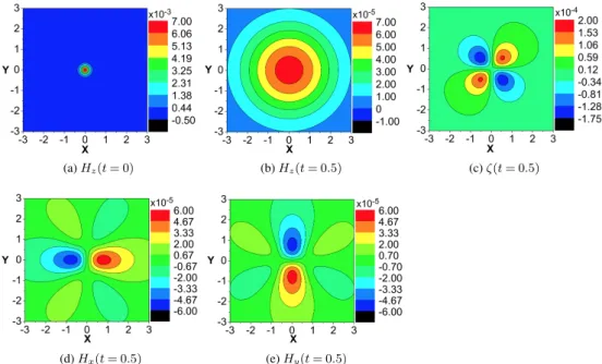
Fig. 3.Excitation of PEMW by means of vertical component of magnetic field. Spatial distributions of normalised components of magnetic field(Hx, Hy, Hz)andζ at different times are shown at hightZ=300 km (night-time).X andY are normalised byR=6.4×10³km. Components of magnetic fieldH are normalised byH0=3×10⁴nT. Dimensionless size of the source are1x=0.25 and1y=0.17;
1X0H=1Y0H=0 andθ=0. PEMW was excited by initial perturbation ofHz(Hz(t=0)max=0.01).
F2≡C4bζ+C4cUz+J (Uz, Az)+J (ξ, Hz);
F3≡α0 V
A0 U0
J (HzAz)+α0J (ξ Uz)−γ Uz;
F4≡C7aζ+C7fUz+J (ξ, z)
+α0 VA02
U02 !
J (ζ, Az)−γ z. (31) This system consists of four evolution equations forζ,Hz, Uz, andz, and two Poisson equations forAz andξ. Note that the corresponding system of equations, which includes the coefficientCij in the limitλ→π/2, is presented in the Appendix B. All functions are set to zero at the boundaries of numerical domain. The full numerical box isLx=20Rkm wide andLy=20Rkm high (whereR is the Earth radius). We have chosen a sufficiently big numerical domain to avoid an nonphysical numerical influence (i.e. possible reflection) of the boundaries. To solve the Poisson equations, we applied fast Fourier transform (FFT) (Press et al., 1997).
The evolution equations have been solved by splitting with respect to the physical factors (Marchuk, 1994). This method can be called a spectral – grid Arakawa type method. Specif-ically, the first fractional step in splitting is related to the diffusion-like process (terms1⊥ζ and1⊥Hzin the first and second Eq. 31). To find the functionζ we solved:∂ζ /∂t= C1a1⊥ζ+F1. Before applying FFT, the function F1 has been calculated with finite differences. We kept the same numerical grid(x, y)for the finite differences and for spec-tral FFT. Roache (1998) and Arakawa (1997) have shown that simplest approximations of the spatial derivatives in the
Jacobians are not conservative and may lead to essential er-rors at long times. Therefore, the Arakawa approximation for the Jacobians has been used only at the first fractional step. The second fractional step is related to the convection terms in all evolution equations. For example, for the functionζ it is∂ζ /∂t= − U0x∂ζ /∂x+U0y∂ζ /∂y. Since the wind ve-locitiesU0x,y are at least one order smaller than the Alfvén velocity, the simplest corner-like upwind scheme can be ap-plied there (see e.g. Roache, 1998).
This method demonstrated a good stability and flexibil-ity. This is further development of our techniques proposed before for modelling of solitons and bullets in nonlinear gy-rotropic structures (see e.g. Rapoport et al., 2002; Slavin et al., 2003; Zaspel et al., 2001), and solitons and strongly non-linear waves in metamaterial structures (see e.g. Boardman et al., 2010, 2011a, b; Rapoport et al., 2012a, for details). The conductivities dependence on height and time of the day has been calculated based on data from Alperovich and Fedorov (2007) (see Fig. 2a). Based on that, we found coefficientsq1, q2 which are included in the RHS of the first four parts of Eqs. (17) (see also relations (18)–(24) and Appendix A). The height dependence of theq1,q2is shown in Fig. 2b.
During each simulation PEMW was excited by initial per-turbation of the vertical components of magnetic vortex ζ and magnetic fieldHz. The spatial distributions of these func-tions in the form of Gaussian are as follows:
ζ (t=0)=ζ (t=0)maxexp "
− x
1xζ 2
− y
1yζ 2#
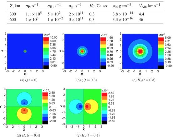
Table 1.The ionosphere night-time parameters.
Z, km σP, s−1 σH, s−1 σ||, s−1 H0, Gauss ρ0, g cm−3 VA0, km s−1
300 1.1×10⁵ 5×10² 2×10¹¹ 0.3 3.8×10⁻¹⁴ 4.4 600 1×10³ 1×10⁻² 3×10¹¹ 0.3 3.3×10⁻¹⁶ 46
(a)ζ(t= 0) (b)ζ(t= 0.3) (c)Hz(t= 0.3)
(d)Hx(t= 0.4) (e)Hy(t= 0.4)
Fig. 4.Excitation of PEMW by means of vertical component of magnetic vortex. The spatial distributions of normalisedζand components of magnetic field(Hx, Hy, Hz)are taken at hightZ=300 km (night-time). Amplitudes of initial excitations are equal toζ (t=0)max=0.01 andHz(t=0)max=0. Dimensionless size of the source are1xζ =1yζ=0.17. The scaling ofX,Y and normalised values ofH are the same as in Fig. 3.
Hz(t=0)=Hz(t=0)maxexp "
− 1x
0H+xcos(θ ) 1xζ
2
− 1y
0H+ysin(θ ) 1yζ
2# .
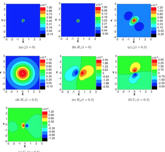
Hereζ (t=0)max,Hz(t=0)maxand1xζ,1yζ are the max-imum values and widths of spatial distributions inX,Y di-rections for ζ and Hz, respectively. 1x0H, 1y0H are the shift values of the maximum of Hz distribution from the coordinate system origin (which coincides with the pole) andθ is the rotation angle in respect to theX axis. Ifθ is equal to zero, the corresponding axis coincides withXaxis. In this section, we consider the excitations of PEMW by means of vertical component of magnetic vortex (ζ (t=0)6= 0,Hz(t=0)max=0 see Figs. 4, 6), vertical component of magnetic field (Hz(t=0)max6=0,ζ (t=0)=0, see Fig. 3), and both vertical components of magnetic field and vortex (Hz(t=0)max6=0, ζ (t=0)6=0, see Fig. 5). Only in the last case, the shifted spatial distribution of the magnetic field is used (1x0H6=0, 1y0H6=0, θ6=0). Corresponding val-ues of amplitudes, shifts and angle are shown in the captions to Figs. 3–6.
(a)ζ(t= 0) (b)Hz(t= 0) (c)ζ(t= 0.3)
(d)Hz(t= 0.3) (e)Hy(t= 0.3) (f)Ux(t= 0.3)
(g)Uz(t= 0.5)
Fig. 5.The spatial distributions of normalised magnetic vortexζ, components of magnetic field(Hy, Hz)and velocity(Ux, Uz)are taken at hightZ=300 km (night-time). PEMW was excited by initial perturbation ofHzandζ (Hz(t=0)max=0.05 andζ (t=0)max=0.05). For the case(g)Hz(t=0)max=0.03 andζ (t=0)max=0.03. For(a–f)1xζ=1yζ=0.17,1xH=1yH=0.17;1x0H=1y0H=0 and
θ=0; for(g)1xζ=1yζ=0.35,1xH=1yH=0.25;1x0H=1y0H=0.2 andθ=45◦. The scaling ofX,Y and normalised values of
Hare the same as in Fig. 3. The velocity componentUzis normalised byVA=4.4 km s−1.
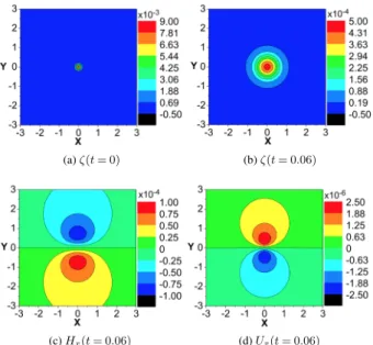
day conditions, the values of magnetic field perturbations are about half of order less than at night, because the Pedersen conductivity in F region at night is larger and the effective diffusion, respectively, smaller, than at daytime (Alperovich and Fedorov, 2007). The PEMW excited by the pulse-like initial perturbation can exist for about∼500 s (see Figs. 3– 5) and even up to 103s, for the heights withinF region of the ionosphere. At higher height (i.e. at Z=600 km) the characteristic time for retain PEMW is smaller (i.e.<102s). This is due to the smaller value of the Pedersen conductiv-ity σP∼103s−1and higher Alfvén speed. Excitations of PEMW at daytime atZ=600 km are negligibly small and not shown here.
The results are presented for the initial normalised value of the magnetic fieldH¯z=0.01, what corresponds to a dimen-sional value Hz∼100 nT, that is possible for PEMW vor-tices (Aburjania et al., 2005). The chosen value of normalised vortex ζ¯=(curlH)z∼0.01 means that the corresponding
(a)ζ(t= 0) (b)ζ(t= 0.06)
(c)Hx(t= 0.06) (d)Ux(t= 0.06)
Fig. 6.The spatial distributions of normalisedζ,HxandUx compo-nents of magnetic field and velocity are taken at hightZ=600 km (night-time). PEMW was excited by vertical component of mag-netic vortexζz(ζ (t=0)max=0.01). The scaling ofX,Y and nor-malised value ofHxis the same as in Fig. 3. The velocity compo-nentUxis normalised byVA=46 km s−1.
the excited PEMW also depend on the type of initial pertur-bations. In particular, an initial perturbation in the form of a bell-like vertical component of the magnetic vortex (Fig. 4a) leads to the formation of the same shape of vertical magnetic field (Fig. 4c). An excitation by means of the initial bell-like vertical component of the magnetic field (Fig. 3a) results in a quadrupole magnetic vortex (Fig. 3c). The combined excita-tion by means of initial vertical components of both magnetic field and vortex (Fig. 5a–c) cases, besides a simple deforma-tion of the horizontal components of the magnetic field and velocities (Fig. 5c, e, f) causes, also a qualitative change in the shape ofζ. Precisely, the spatial distribution of ζ pos-sesses two “dips”, around the central maximum (Fig. 5c).
Figure 5g demonstrates a new and interesting behaviour of velocityUzatZ=300 km, during night-time conditions, with a remarkable nonlinearity and due to a presence of combined source; that is, if both Hz and ζ are present at t=0. We use the initial perturbations of normalisedHzand ζ with maximum values equal to 0.05, which corresponds to a magnetic field of order of 1000 nT. However this rather extreme value is still in a range of possible amplitudes for PEMW vortex structures and in agreement with evaluations by Aburjania et al. (2005). The corresponding value of the vertical current is of order ofJ ∼3×10⁻⁷A m−2. Based on results which are shown on Fig. 5g, we can conclude, that under such conditions, a vertical displacement of a medium during a characteristic time of order of 103s reaches the value of order of 100 m. However, the vertical displacement corresponding to the combined sources at Z=600 km is
negligibly small (not shown here). Note that in case of com-bined source (i.e. bothHz andζ), the nonlinear “effective source” of excitation of Uz in the near-pole region is pro-vided, which is evident from Eq. (B3). It is further recalled that, at the middle latitudes, both linear and nonlinear exci-tations of the vertical velocity component are possible (see the third Eq. 17 and relation 22). A rough estimation shows that the vertical displacement at heightZ=300 km reaches a value of the order of 1 km. We have found that, within the ionosphere F region (i.e. at Z=300 km) the pulse-like PEMW can retain their structure up to 103s. At the higher al-titudes (Z=600 km) PEMW could only be observed during the night-time and they preserve their shapes up to 102s due to the much smaller Pedersen conductivity in the magneto-sphere than in the ionomagneto-sphere. The magnetic field of PEMW has the characteristic values:Hzof the order of one to a few nT, Hx,y of the order of a few to 10 nT. These values are well above the sensitivity of the modern magnetometers, and therefore, they can be detected (Prattes et al., 2011, see also Sect. 7).
7 Discussion and conclusions
effort, since speed is low, that is combined with the relatively small magnitudes of these displacements. Here it is appro-priate to provide selected data on the possibilities of relevant methods for ionospheric disturbances measurements. The DOPE (Doppler Pulsation Experiment) HF Doppler sounder located near Tromsø, Norway has a spatial resolution of the order of 4 km, for F region reflection height of 250 km and a sounder frequency of 4.45 MHz (see e.g. Wright et al., 1997). The method of GPS differential TEC (see e.g. Borries et al., 2007) has a spatial resolution of about 50–100 m. At last, the CHInese MAGnetometer (CHIMAG) fluxgate magnetome-ter chain has an accuracy of 8 pT at a temporal resolution of 1 Hz (see e.g. Prattes et al., 2011). The spatial dimensions of the objects under consideration and vertical displacements are of the order of 1000 km and 1 km, respectively, and the magnetic fields are of the order of 10 nT at a frequency of about 0.01 Hz. In view of this it can be concluded that based on the multipoint synchronised measurements using differ-ential GPS TEC and chains of magnetometers and advanced data processing methods, it is possible to identify PEMWs in the ionosphere.
It should be noted that large-scale experiments to study the phenomenon of PEMW have not been carried out yet. And this, despite the fact that, according to Aburjania et al. (2005), PEMWs are natural ionospheric oscillations, and therefore, they are a primary link in the chain of the iono-sphere’s response to disturbances both from below and from above (earthquakes, hurricanes, high-frequency ionosphere heating, magnetosphere’s and solar wind impacts).
The theoretical background of relevant experiments, there-fore, includes (a) classification of various modes of hydro-magnetic waves in the ionosphere (Aburjania et al., 2002, 2003b; Aburjania and Chargazia, 2011); (b) estimations of wave parameters in linear theory (Aburjania et al., 2002, 2003b; Rapoport et al., 2007; Aburjania and Chargazia, 2011); and (c) systematisation of estimates to prepare a mea-surement scheme (Aburjania et al., 2002, 2003b; Aburjania and Chargazia, 2011). In particular, it has been found that the phase speed is of the order of 1 km s−1to 103km s−1and even higher, depending on height, while the wavelength is of order 103to 104km. The most promising estimate relates to the magnitude of magnetic disturbances caused by PEMW: it is of the order of up to 102nT and in certain cases – up to 103nT in situ for vortex structures propagating along the F layer (Aburjania et al., 2005).
There are a number of experiments devoted to mea-surements of the excitation of ULF hydromagnetic waves by different sources in the ionosphere (see e.g. Burmaka et al., 2006). Wave disturbances of the geomagnetic field associated with distant rocket launches were measured us-ing the modified ionosonde “Basis”, the fluxgate magne-tometer, and the radar of incoherent scattering at the Iono-sphere observatory, near Kharkov, Ukraine. In total, mea-surements of ionospheric wave disturbances from about 140 distant missile launches were carried out for about 10 yr.
The observations were made at various distances from the launching sites (Baikonur, Plesetsk, et al.): from 700 km to about 104km. It was found that (a) perturbations with a speed of 10–20 km s−1are quite often observed at distances of up to 2300 km from the rocket; (b) there were 3 groups of speeds of disturbances: 0.5–0.7 km s−1, 2–3 km s−1, and 10–25 km s−1; (c) there were 3 groups of periods of domi-nant geomagnetic micropulsations: about 6, 10, and 20 min, their amplitudes on the ground attained a value of 3–5 nT; (d) the launch-resulted waves were most pronounced at altitudes 150–350 km; (e) relative amplitudes of disturbances of the electron concentration reached 5–7 %. The analysis of such observations shows that the difficulty in identifying waves is that the frequencies of typical PEMW packets belong to the ULF band and may be buried in the noise that exists there. To be able to detect PEMW packets in this background, it seems possible to use sophisticated data analysis techniques that have worked well in the study of seismic and oceanic wave processes: directional spectra estimation (see e.g. Sun et al., 2005); study of a packet modification due to the co-action of nonlinearity, dispersion, and dissipation; using the concept of so called “coda waves” (see e.g. Sèbe et al., 2005). These techniques become more efficient when we take into account the internal multi-scale nature of the processes under study. For example, wavelet packet transform where appro-priate statistical decision rule is applied to subset of wavelet coefficients (Lyubushin, 2007) gives a tool to detect complex changes, say, in magnetometer recordings.
Finally, it should be emphasised that the present state of theoretical and modelling studies in the area of PEMW puts on the agenda the question of systematic experiments on the identification of PEMWs under various geomag-netic conditions, on revealing their sources, correlations with space weather events and catastrophic events throughout the atmosphere–ionosphere system. This requires the organisa-tion of measurements accounting for the large-scale (103– 104km) character of the PEMWs on the base of a planetary size network of ionospheric/magnetospheric observatories.
The proposed theory can be extended by includ-ing the connection between particular couplinclud-ing processes in the “magnetosphere–ionosphere–atmosphere–lithosphere (MIAL)” system and corresponding sources of full-spectrum MHD waves/PEMW in the form of the effective “external currents/fields”.
Here we sum up the results of the present work.
2. A new numerical method for the simulations of the evolution of PEMW is developed. This is a highly stable and efficient hybrid finite difference-spectral method, based on splitting by physical factors. 3. The shapes of the excited PEMW depend on the types
of initial conditions or sources. In particular, the exci-tation of PEMW by an initial bell-like vertical compo-nent of the magnetic vortex leads to the formation of a bell-like vertical magnetic field. The excitations by means of an initial bell-like vertical component of the magnetic field results in a quadrupole magnetic vortex. 4. We have found that diffusion processes are rather im-portant in the spreading of PEMW excitation in the F region of the ionosphere, while in most previous papers, such as Aburjania et al. (2005), this factor was underestimated. The vertical component of the velocity of PEMW is not essential for an altitude of Z=600 km. At altitudeZ=300 km this compo-nent provides a vertical displacement of∼100 m on a timescale∼103s at the high latitudes, while the esti-mate of vertical displacement is∼1 km at the middle latitudes, where both linear and nonlinear wave excita-tion of PEMW is possible.
5. The components of the magnetic field of PEMW are of the order of one to a few nT for the vertical com-ponent and from a few to tens of nT for the horizontal component; therefore, it can be measured by modern instruments.
Future practical applications of the model described here may include detection of PEMWs and other MHD waves in the context of a space weather monitoring system.
Acknowledgements. This research is partially supported by Royal Society International Exchanges Scheme and RFBR under grant 13-05-92602 KOa. The paper have been supported by Comprehensive program of NAS of Ukraine on Space Research.
Topical Editor M. Gedalin thanks J. De Keyser and one anony-mous referee for their help in evaluating this paper.
References
Aburjania, G. D. and Chargazia, Kh. Z.: Self-organization of large-scale ULF electromagnetic wave structures in their interaction with nonuniform zonal winds in the ionospheric E region, Plasma Phys. Rep., 37, 177–190, doi:10.1134/S1063780X10111017, 2011.
Aburjania, G. D., Khantadze, A. G., and Kharshiladze, O. A.: Nonlinear Planetary Electromagnetic Vortex Structures in the Ionospheric F-Layer, Plasma Phys. Rep., 28, 586–591, doi:10.1134/1.1494057, 2002.
Aburjania, G. D., Jandieri, G. V., and Khantadze, A. G.,: Self-organization of planetary electromagnetic waves in the E-region of the ionosphere, J. Atmos. Sol.-Terr. Phys., 65, 661–671, doi:10.1016/S1364-6826(03)00003-8, 2003a.
Aburjania, G. D., Khantadze, A. G., and Gvelesiani, A. I.: Physics of generation of the new branches of planetary electromagnetic waves in the ionosphere, Geomagn. Aeron., 42, 193–203, 2003b. Aburjania, G. D., Chargazia, Kh. D., Jandieri, G. V., Khantadze, A. G., Kharshiladze, O. A., and Lominadze, J. D.: Generation and propagation of the ULF planetary-scale electromagnetic wave structures in the ionosphere, Planet. Space Sci., 53, 881–901, doi:10.1016/j.pss.2005.02.004, 2005.
Alperovich, L. S. and Fedorov, E. N.: Hydromagnetic Waves in the Magnetosphere and the Ionosphere, Astrophysics and Space Sci-ence Library, Springer, Vol, 353, 425 pp., 2007.
Arakawa, A.: Self-organization of planetary electromagnetic waves in the E-region of the ionosphere, Computational Design for Long-Term Numerical Integration of the Equations of Fluid Mo-tion: Two-Dimensional Incompressible Flow. Part I, J. Comput. Phys., 135, 103–114, doi:10.1006/jcph.1997.5697, 1997. Boardman, A. D., Hess, O., Mitchell-Thomas, R., Rapoport, Y.
G., and Velasco, L.: Temporal solitons in magnetooptic and metamaterial waveguides, Photonic. Nanostruct., 8, 228–243, doi:10.1016/j.photonics.2010.05.001, 2010.
Boardman, A. D., Grimalsky, V. V., and Rapoport, Yu. G.: The hybrid method of nonlinear transformational and complex geo-metrical optics for energy concentration in metamaterials, Meta-materials 2011: The Fifth International Congress on Advanced Electromagnetic Materials in Microwaves and Optics, Barcelona, 763–765, 2011a.
Boardman, A. D., Grimalsky, V. V., and Rapoport, Yu. G.: Nonlinear transformational optics and electromagnetic and acoustic fields concentrators, The Fourth International Workshop on Theoretical and Computational Nanophotonics, AIP Conf. Proc., 1398, 120– 122, 2011b.
Burmaka, V. P., Lysenko, V. N., Chernogor, L. F., and Chernyak, Yu. V.: Wave-Like Processes in the Ionospheric F Region that Ac-companied Rocket Launches from the Baikonur Site, Geomagn. Aeron., 46, 783–800, 2006.
Borries, C., Jakowski, N., Jacobi, Ch., Hoffmann, P., and Pogorelt-sev, A.: Spectral analysis of planetary waves seen in ionospheric total electron content (TEC): First results using GPS differential TEC and stratospheric reanalyses, J. Atmos. Sol.-Terr. Phys., 69, 2442–2451, doi:10.1016/j.jastp.2007.02.004, 2007.
Clark, R. M., Yeh, K. C., and Liu, C. H.: Interaction of internal grav-ity waves with the ionospheric F2-layer, J. Atmos. Terr. Phys., 33, 1567–1576, doi:10.1016/0021-9169(71)90074-2, 1971. Gill, A. E.: Atmosphere-Ocean Dynamics, Academic Press,
662 pp., 1982.
Guglielmi, A. V. and Pokhotelov, O. A.: Geoelectromagnetic waves, Taylor & Francis, Bristol, 382 pp., 1996.
Herron, T. J.: Phase Characteristics of Geomagnetic Micropulsations, J. Geophys. Res., 71, 871–889, doi:10.1029/JZ071i003p00871, 1966.
Kaladze, T. D., Pokhotelov, O. A., Sagdeev, R. Z., Stenflo, L., and Shukla, P. K.: Planetary electromagnetic waves in the ionospheric E-layer, J. Atmos. Sol.-Terr. Phys., 65, 757–764, doi:10.1016/S1364-6826(03)00042-7, 2003.
Khantadze, A. G.: Some questions of the dynamics of the conduct-ing atmosphere, Metsniereba, Tbilisi, 1973 (in Russian). Landau, L. D., Pitaevskii, L. P., and Lifshits, E. M.:
Theoretical Physics), Elsevier Butterworth-Heinemann, Oxford, 460 pp., 2004.
Lyubushin, A. A.: Geophysical Monitoring Systems Data Analysis, Moscow, Nauka, 228 pp., 2007 (in Russian).
Marchuk, G. I.: Numerical Methods and Applications, 1st Edn., CRC Press, Boca Raton, 288 pp., 1994.
Onishchenko, O. and Pokhotelov, O.: Generation of zonal structure by internal gravity waves in the Earths At-mosphere, Doklady Earth Sciences, 445, 845–848, doi:10.1134/S1028334X12070070, 2012.
Onishchenko, O., Pokhotelov, O., and Astafieva, N.: Gen-eration of large-scale eddies and zonal winds in plan-etary atmospheres, Physics-Uspekhi, 51, 577–589, doi:10.1070/PU2008v051n06ABEH006588, 2008.
Onishchenko, O., Pokhotelov, O., and Fedun, V.: Convective cells of internal gravity waves in the earth’s atmosphere with finite temperature gradient, Ann. Geophys., 31, 459–462, doi:10.5194/angeo-31-459-2013, 2013.
Pilipenko, V. A., Shalimov, S. L., Fedorov, E. N., Engebretson, M. J., and Hughes, W. J.: Coupling between field-aligned current impulses and Pi1 noise bursts, J. Geophys. Res., 104, 17419– 17430, doi:10.1029/1999JA900190, 1999.
Prattes, G., Schwingenschuh, K., Eichelberger, H. U., Magnes, W., Boudjada, M., Stachel, M., Vellante, M., Villante, U., Weszter-gom, V., and Nenovski, P.: Ultra Low Frequency (ULF) Eu-ropean multi station magnetic field analysis before and during the 2009 earthquake at L’Aquila regarding regional geotechni-cal information, Nat. Hazards Earth Syst. Sci., 11, 1959–1968, doi:10.5194/nhess-11-1959-2011, 2011.
Press, W. H., Teukolsky, S. A., Vetterling, W. T., and Flannery, B. P.: Numerical Recipes in Fortran 77. The Art of Scientific Com-puting, Cambridge Univ. Press, NY, 1997.
Rapoport, Yu. G., Zaspel, C. E., Mantha, J. H., and Grimalsky, V. V.: Multisoliton formation in magnetic thin films, Phys. Rev. B, 65, 244231–244234, doi:10.1103/PhysRevB.65.024423, 2002. Rapoport, Yu. G., Gotynyan, O. E., Ivchenko, V. M., Kozak, L.
V., and Parrot, M.: Effect of acoustic-gravity wave of the litho-spheric origin on the ionolitho-spheric F region before earthquakes, Phys. Chem. Earth, 29, 607–616, doi:10.1016/j.pce.2003.10.006, 2004.
Rapoport, Yu. G., Kotsarenko, A. N., Agapitov, A. V., Milinevsky, G. P., and Selivanov, Yu. A.: Planetary electromagnetic waves (PEMW) in the ionospheric region F, in: 7th Ukrainian Confer-ence on Space Research, 4–7 September 2007, Crimea, Evpato-ria, Ukraine, Abstracts, 98, 2007.
Rapoport, Yu. G., Hayakawa, M., Gotynyan, O. E., Ivchenko, V. N., Fedorenko, A. K., and Selivanov, Yu. A.: Stable and unstable plasma perturbations in the ionospheric F region, caused by spa-tial packet of atmospheric gravity waves, Phys. Chem. Earth, Pt. A/B/C, 6–7, 508–515, doi:10.1016/j.pce.2008.09.001, 2009. Rapoport, Yu. G., Cheremnykh, O. K., Selivanov, Yu. A.,
Fe-dorenko, A. K., Ivchenko, V. M., Grimalsky, V. V., and Tkachenko, E. N.: Oscillations of neutral and charged com-ponents of near-Earth plasma and effects of active media, in: UK-Ukraine Meeting on Solar Physics and Space Science UKU SPSS/TASS-2011, 29 August–2 September, 2011 Alushta, Crimea, Ukraine, PROGRAMME and ABSTRACTS, 69, 2011. Rapoport, Yu., Boardman, A., Grimalsky, V., Selivanov, Yu., and
Kalinich, N.: Metamaterials for space physics and the new
method for modeling isotropic and hyperbolic nonlinear con-centrators, in: Mathematical Methods in Electromagnetic Theory (MMET), 2012 International Conference, 76–79, 2012a. Rapoport, Yu. G., Cheremnykh, O. K., Selivanov, Yu. A.,
Fe-dorenko, A. K., Ivchenko, V. M., Grimalsky, V. V., and Tkachenko, E. N.: Modeling AGW and PEMW in inhomoge-neous atmosphere and ionosphere, in: Mathematical Methods in Electromagnetic Theory (MMET), 2012 International Confer-ence, IEEE, 577–580, 2012c.
Roache, P. J.: Fundamentals of Computational Fluid Dynamics, Hermosa Publ., NY, 648 pp., 1998.
Saliuk, D. A. and Agapitov, O. V.: Vortex and ULF wave structures in the plasma sheet of the Earth magnetosphere, Advances in As-tronomy and Space Physics, 3, 53–57, 2013.
Saliuk, D. A., Agapitov, O., and Milinevsky, G. P.: Magnetized Rossby waves in mid-latitude ionosphere F-layer, Advances in Astronomy and Space Physics, 2, 95–98, 2012.
Sèbe, O., Bard, P.-Y., and Guilbert, J.: Single station esti-mation of seismic source time function from coda waves: The Kursk disaster, Geophys. Res. Lett., 32, L14308, doi:10.1029/2005GL022799, 2005.
Slavin, A. N., Büttner, O., Bauer, M., Demokritov, S. O., Hille-brands, B., Kostylev, M. P., Kalinikos, B. A., Grimalsky, V. V., and Rapoport, Yu.: Collision properties of quasi-one-dimensional spin wave solitons and two-quasi-one-dimensional spin wave bullets, Chaos, 13, 693–701, doi:10.1063/1.1557961, 2003. Sorokin, V. M. and Fedorovich, G. V.: Physics of Slow MHD Waves
in the Ionospheric Plasma, Energoizdat, Moscow, 1982 (in Rus-sian).
Southwood, D. J. and Kivelson, M. G.: Vortex motion in the iono-sphere and nonlinear transport, J. Geophys. Res., 98, 11459– 11466, doi:10.1029/93JA00434, 1993.
Sun, J., Burns, S. P., Vandemark, D., Donelan, M. A., Mahrt, L., Crawford, Timothy, L., Herbers, T. H. C., Crescenti, G. H., and French, J. R.: Measurement of Directional Wave Spectra Using Aircraft Laser Altimeters, J. Atmos. Ocean. Tech., 22, 869–885, doi:10.1175/JTECH1729.1, 2005.
Szegö, K., Glassmeier, K.-H., Bingham, R., Bogdanov, A., Fischer, C., Haerendel, G., Brinca, A., Cravens, T., Dubinin, E., Sauer, K., Fisk, L., Gombosi, T., Schwadron, N., Isenberg, P., Lee, M., Mazelle, C., Möbius, E., Motschmann, U., Shapiro, V. D., Tsuru-tani, B., and Zank, G.: Physics of Mass Loaded Plasmas, Space Sci. Rev., 94, 429–671, doi:10.1023/A:1026568530975, 2000. Tolstoy, I.: Hydromagnetic Gradient Waves in the Ionosphere, J.
Geophys. Res., 72, 1435–1442, doi:10.1029/JZ072i005p01435, 1967.
Verkhoglyadova, O. P., Agapitov, A. V., and Ivchenko, V. N.: Model of vortex tubes in the low-latitude plasma sheet of the Earth mag-netosphere, Adv. Space Res., 28, 801–806, doi:10.1016/S0273-1177(01)00511-7, 2001.
Wright, D. M., Yeoman, T. K., and Chapman, P. J.: High-latitude HF Doppler observations of ULF waves. 1. Waves with large spatial scale sizes, Ann. Geophys., 15, 1548–1556, doi:10.1007/s00585-997-1548-2, 1997.
Appendix A
The coefficient included in general set of equations for PEMW (17)–(24)
The coefficients included in general set of equations for PEMW (17)–(24) are
C1a=s0 h
1−< h20z>i; C1b= −s0q2h0yh0z; C1c=2s0q1
∂h0y ∂y ;
C1d= −s0q1
2 ∂
∂y h0yh0z − ∂ ∂zh 2 0y ;
C1e=s0q1h0y; C1f =s0q1 ∂h0y
∂z ; (A1)
C1g=s0q1 ∂h0z
∂z ; C1h= −s0q2 ∂
∂z h0zh0y
−2 ∂ ∂yh
2 0z
;
C2a= −α0H0y;
C2b= −2α0 ∂H0y
∂y ; C2c=α0 ∂H0z
∂z ;
C2d= −α0 ∂H0y
∂z ; C2e= −2α0 ∂H0y
∂y ;
C3a=α0; s0=α02
(c/U0)2 4π σeff ;
(A2) C4a=s0; C4b= −s0q1
∂h0y
∂y ; C4c=α0 ∂H0y
∂y ;
C4d= −s0q1h0y; C4e= −s0q1 ∂h0z
∂y ; C4f = −s0q2h 2 0y;
C4g= −s0h0yh0z;
C5a=α0H0y; C5b=α0 ∂Hz0
∂y ; C5c=α0 ∂H0y
∂y ; (A3) C6a=α0
V A0 U0
2
H0y; C6b=(0sct0)20y; (A4)
C7a=α0 V
A0 U0
2∂H 0y
∂y ; C7b=α0 V A0 U0 2∂H 0z ∂y ;
C7c=α0 V
A0 U0
2
H0y; C7d=
∂(20z) ∂y ;
C7e=20y; C7f =
∂ 20y
∂y . (A5)
Here0sc andU0 are scales of angular frequency and ve-locity, respectively.α0=VL0t0
0 , whereV0,t0andL0are char-acteristic scales of velocity, time and length. Note that the value< h20z>is a phenomenologically averaged value of the square of the directional vector componenth20zin the region of existence of PEMW perturbation located in a region near a pole (but not exactly on a pole). Due to< h20z> <1, the termC1a>0, thus providing damping ofζ(see first equation in Eqs. 17).
Appendix B
Equations for the near-pole region
For the near-pole region, we obtain from Eqs. (17)–(24) with the coefficients determined by formulae (A1)–(A5) in the limitλ→π/2, the set of equations:
Dtζ =α02 (c/ϑ0)2 4π σeff
11ζ
1+q2
D
h20zE+2q1 ∂h0y
∂y ∂2hz
∂y2
−2q2
∂ h0zh0y
∂y
∂2hz ∂x∂y
)
+ +α01⊥J Az,ξ
−2α0 ∂H0y
∂y ∂2ξ ∂y2+α0
∂H0z
∂z z; (B1)
DtHz=α20
(c/U0)2 4π σeff
1⊥Hz−q1 ∂h0y
∂y ζ
+α0 ∂H0y
∂y Uz +α0J (Uz, Az)+α0J (ξ, Hz); (B2) DtUz=α0
V A0 U0
2
J (Hz, Az)+α0J (ζ, Uz)−γ Uz;(B3)
Dtz=α0 V
A0 U0
2∂H 0y ∂y ζ+2
∂0y
∂y Uz+J (ζ, Uz)
+α0 V
A0 U0
2
J (ζ, Az)−γ z; (B4) 1⊥Az= −ζ; 1⊥ξ = −z. (B5) Here
∂H0z ∂z =
Heq R = −
∂H0y ∂y ; ∂0y ∂y = 0 R ; ∂h0y
∂y = − 1 2R;
∂2H0y
∂y∂z = 2Heq
R2 ; ∂2h0z
∂y2 = − 1 2R2; h0z=1;
∂ h0zh0y
∂y =
1 2R.
Appendix C
Equations for the near-equator region
In the near-equator region, we obtain the following set of nor-malised equations from the system of Eqs. (17) accounting for the relations (18)–(24) in the limiting caseλ→0:
Dtζ =α02
(c/U0)2 4π σeff
Q+α01⊥J (Az, ξ )
−α0 "
H0y1⊥ ∂ξ ∂y+
∂H0y2
∂y2 ∂2ξ ∂y2+
∂H0y ∂z ∂Uz ∂x # ; (C1)
DtHz=α20
(c/U0)2 4π σeff
1⊥Hz−q1 h0y ∂ζ ∂y + ∂h0z ∂y ∂Hz ∂x
+q2h20y ∂2Hz
∂x2
+α0J (Uz, Az)+α0J (ξ, Hz); (C2) DtUz=
" α0
V A0 U0
2 H0y
∂Hz
∂y +200y ∂ξ ∂y
#
+ "
α0 V
A0 U0
2
J (Hz, Az)+α0J (ξ, Uz) #
−γ Uz; (C3)
Dtz=α0 V
A0 U0
2∂H 0y ∂y¯
∂Hz ∂x¯ +H0y
∂ζ ∂y
+
2∂0z ∂y
∂ξ
∂x+20y ∂Uz
∂x
+J (ξ, z)+α0 V
A0 U0
2
J (ζ, Az)−γ z; (C4) 1⊥Az= −ζ; 1⊥ξ = −z, (C5) where
Q=1⊥ζ−q1
15 R2
∂Hz
∂x − ∂
∂y1⊥Hz
+q2
11 R2ζ+
4 R
∂2Hz ∂x∂y
;
H0y=Heq; ∂H0z
∂y = − 2Heq
R ; ∂20z
∂y = 20
R ;
0y=0 ∂H0y
∂z = − 2Heq
R ; ∂h0z
∂y = − 2 R;
∂H0z ∂y = −
2Heq