I. Maiello1, R. Ferretti1,2, S. Gentile1, M. Montopoli1,3, E. Picciotti1,4, F. S. Marzano1,3, and C. Faccani5
1Centre of Excellence CETEMPS, L’Aquila, Italy
2Department of Physical and Chemical Sciences, University of L’Aquila, L’Aquila, Italy
3Department of Information Engineering, Electronics and Telecommunications, Sapienza University of Rome, Rome, Italy 4HIMET s.r.l., L’Aquila, Italy
5ENAV S.p.A. – Academy, Forlì, Italy
Correspondence to:I. Maiello ([email protected], [email protected]) Received: 15 March 2013 – Published in Atmos. Meas. Tech. Discuss.: 8 August 2013 Revised: 1 August 2014 – Accepted: 5 August 2014 – Published: 12 September 2014
Abstract. The aim of this study is to investigate the role of the assimilation of Doppler weather radar (DWR) data in a mesoscale model for the forecast of a heavy rainfall event that occurred in Italy in the urban area of Rome from 19 to 22 May 2008. For this purpose, radar reflectivity and radial velocity acquired from Monte Midia Doppler radar are assimilated into the Weather Research Forecasting (WRF) model, version 3.4.1. The general goal is to improve the quantitative precipitation forecasts (QPF): with this aim, sev-eral experiments are performed using the three-dimensional variational (3DVAR) technique. Moreover, sensitivity tests to outer loops are performed to include non-linearity in the observation operators.
In order to identify the best initial conditions (ICs), sta-tistical indicators such as forecast accuracy, frequency bias, false alarm rate and equitable threat score for the accumu-lated precipitation are used.
The results show that the assimilation of DWR data has a large impact on both the position of convective cells and on the rainfall forecast of the analyzed event. A positive impact is also found if they are ingested together with conventional observations. Sensitivity to the use of two or three outer loops is also found if DWR data are assimilated together with con-ventional data.
1 Introduction
The initial conditions (ICs) are a key term for a success-ful forecast performed using a high-resolution numerical weather prediction (NWP). Generally, localized mesoscale features are not well represented in the ICs. The assimila-tion of local observaassimila-tions into the ICs may produce a fore-cast improvement. In the last 80 years, different methods of data assimilation have been investigated: the successive cor-rections method (SCM), the optimal interpolation (OI), the variational methods 3DVAR and 4DVAR, and the Kalman fil-ter (KF) are some notable examples. During the last decade, high-resolution mesoscale models initialized using varia-tional data assimilation techniques (3DVAR/4DVAR) are be-ing increasbe-ingly applied to study meteorological phenomena (Kalnay, 2003). One of the reasons for the variational anal-ysis becoming more and more popular is the ability to di-rectly incorporate some non-conventional observations such as satellite radiance, radar reflectivity and radial velocity into numerical models (Kalnay, 2003; Barker et al., 2004), through the use of a proper operator.
2920 I. Maiello et al.: Impact of radar data assimilation using WRF-3DVAR
velocity has shown the potential for very short-range numer-ical weather prediction of rapidly developing convective sys-tems. It is well known that reflectivity is related to the num-ber of falling drops per unit volume, and it depends on the number and size of hydrometeors, whereas the vertical com-ponent of radial velocity contains information on vertical at-mospheric motions. Both are important for the triggering and development of convection. However, radial velocity’s con-tribution to its vertical component is variable, and it depends on the elevation of the radar antenna and variations in the atmospheric refractive index. The latter might produce vari-ations in the radar ray paths with respect to those expected under standard atmosphere conditions. In this work, a stan-dard atmosphere is assumed, and this means that radar ray paths propagate in a straight line (Bech et al., 2003).
The first radar data assimilation system for the storm scale was developed based on the four-dimensional varia-tional data assimilation (4DVAR) technique and a bound-ary layer fluid dynamics model for the retrieval of the three-dimensional wind and temperature (Sun et al., 1991). This system, known as VDRAS (the Variational Doppler Radar Analysis System), was later expanded to include microphys-ical retrieval, as well as short-term forecasts initialized by these retrieved fields (Sun and Crook, 1997, 1998). Another variational-based radar data assimilation system was devel-oped by Gao et al. (2004) using a three-dimensional varia-tional data assimilation (3DVAR) technique in the framework of the ARPS (Advanced Research and Prediction System, Xue et al., 2003) model. A so-called 3.5-dimensional varia-tional radar data assimilation based on the navy’s COAMPS (Coupled Ocean/Atmosphere Mesoscale Prediction System) was developed and verified through a number of studies (Zhao et al., 2006; Xu et al., 2010). These variational systems showed great potential in the use of radar observations for initializing high-resolution numerical models through sev-eral case studies and real-time demonstrations (Sun et al., 2010; Xue et al., 2010).
These results motivated the development of a radar data as-similation scheme in the WRFVAR variational data assimila-tion system of the ARW-WRF (Advanced Research Weather Research and Forecasting) community model.
The operators for radial velocity (Xiao et al., 2005) and reflectivity (Xiao et al., 2007; Xiao and Sun, 2007) data were added to the three-dimensional variational data as-similation system (Barker et al., 2003, 2004; Skamarock et al., 2008) developed at the National Center for Atmo-spheric Research (NCAR) laboratories for both the fifth-generation Penn State/NCAR Mesoscale Model (MM5) and the Weather Research Forecasting (WRF) model. WRFVAR includes both 3DVAR and 4DVAR components. The radar DA scheme was first developed for WRF–3DVAR (Xiao et al., 2005, 2007) and recently expanded to 4DVAR (Wang et al., 2013; Sun and Wang, 2012).
Xiao et al. (2005) assimilated radial velocities from a sin-gle Doppler radar into MM5 using the 3DVAR scheme for a heavy rainfall event. The vertical velocity increments were included via Richardson’s balance equation, and an observa-tion operator for radial velocity was developed. The results suggested that the scheme for the radial velocity assimilation is stable and robust in a cycling mode using high-frequency radar data. Moreover, continuous assimilation with 3 h up-date cycles was important for improving heavy rainfall.
A radar reflectivity data assimilation scheme was also de-veloped within the MM5–3DVAR system, as described by Xiao et al. (2007). They showed that the intensity and track of Typhoon Rusa (2002) were better predicted through the combined assimilation of both radar radial velocity and re-flectivity. Xiao and Sun (2007) used the WRF model and its 3DVAR data assimilation module to ingest data from a net-work of Doppler radars in order to study a squall-line convec-tive system. They found that the assimilation of both radial velocity and reflectivity improved the quantitative precipita-tion forecast (QPF) skills with respect to using only one of the two radar variables. Further improvements to QPF were obtained by the assimilation of more than one radar site using the cycling procedure.
A few studies on the impact of radar data assimilation were also performed for the European area using different forecast models: AROME (Application of Research to Op-erations at MEsoscale) in France and HIRLAM (HIgh Res-olution Limited Area Model) in Sweden. Montmerle and Faccani (2009) applied the 3DVAR assimilation technique for assimilating radial velocities from Doppler radars of the French ARAMIS (Application Radar la Météorologie In-fraSynoptique) network. They found a positive impact of radar wind data on the analyses and on precipitation fore-casts. Lindskog et al. (2004) also assimilated radial wind ve-locity. They used the velocity–azimuth display (VAD) tech-nique that provides vertical profiles of horizontal winds from the Doppler radar raw radial wind and the Doppler radar ra-dial wind superobservations (SOs), which is based on spatial averaging. They found improvements in the wind and tem-perature forecasts of the low and middle troposphere using either VAD or SOs data.
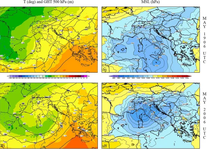
Figure 1.European Center for Medium-Range Weather Forecasts (ECMWF) analyses at 06:00 UTC on 19 May 2008:(a)temperature and geopotential height, at 500 hPa, and(b)mean sea level pressure and surface wind in m s−1; ECMWF analyses at 06:00 UTC on 20 May 2008:
(c)temperature and geopotential height, at 500 hPa, and(d)mean sea level pressure and surface wind in m s−1.
This paper is organized as follows. In Sect. 2, the case study and the radar data used for the assimilation are de-scribed. A brief explanation of the WRF–3DVAR system and the radar data operator is presented in Sect. 3. The 3DVAR experiments and the corresponding forecast results are dis-cussed in Sects. 4 and 5, respectively. The impact of outer loops is analyzed in Sect. 6, whereas summary and conclu-sions are given in Sect. 7.
2 A heavy rainfall case: the meteorological situation From 19 to 22 May 2008, a heavy rainfall event occurred in the urban area of Rome. In the first hours of 19 May, a cyclonic circulation on the southern Mediterranean Sea (Fig. 1b) associated with an intrusion of cold air from Scan-dinavia (Fig. 1a) caused instability on the Italian peninsula. On 20 May, a deep low-pressure system developed in the Genoa Gulf (Fig. 1d), causing severe weather conditions. Southwesterly flow started to blow over the Tyrrhenian Sea, advecting warm and humid air toward the area of Rome (Fig. 1c), further destabilizing the atmosphere.
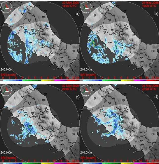
To understand the meteorological evolution of the event better, the surface rainfall intensity (SRI) product (in mm h−1) estimated by the Italian national radar network
(Vulpiani et al., 2008) is shown in Fig. 2. In the early after-noon of 20 May, the precipitation is detected both in the ur-ban area of Rome and over the Tyrrhenian Sea (RM, Fig. 2a). Later, local showers are observed in the southeastern part of RM and over the Tyrrhenian Sea (Fig. 2b). Moderate pre-cipitation lasted until the evening around Rome (Fig. 2c), whereas at 22:00 UTC, the rainfall moved eastward, reach-ing L’Aquila (AQ, Fig. 2d).
3 WRF–3DVAR
3.1 Brief description of WRF–3DVAR
2922 I. Maiello et al.: Impact of radar data assimilation using WRF-3DVAR
Figure 2.Estimated surface rainfall intensity (mm h) by the national radar network in central Italy on 20 May 2008:(a)SRI at 14:00 UTC;
(b)SRI at 16:00 UTC;(c)SRI at 20:00 UTC;(d)SRI at 22:00 UTC. Only the highlighted areas were covered by the national radar network in 2008 (courtesy of the Italian Civil Protection Department).
Figure 3.The panel shows the location of the Monte Midia radar between the Abruzzo (to the right) and Lazio (to the left) regions, its coverage (gray circle), and the rain gauge network (red crosses) used for calibration of the estimated rain.
unbalanced pressurepuand total water mixing ratioqt. The
aim of the three-dimensional variational approach is to pro-duce the best compromise between an a priori estimation of the analysis field and observations through the iterative so-lution that minimizes a cost functionJ. Most leading assim-ilation schemes do not perform the minimization process in the model space, but they use atransformedorcontrol vari-able spacethat is the space allowed for the corrections to the background. This new space is chosen to have a special and desirable property when the background field is represented in this space: its errors are uncorrelated, and variances are of unit size (the problem is said to bepreconditioned).
The cost function for 3DVAR is J (x)=Jb+Jo= 1
2
n
yo−H (x)TR−1yo−H (x)
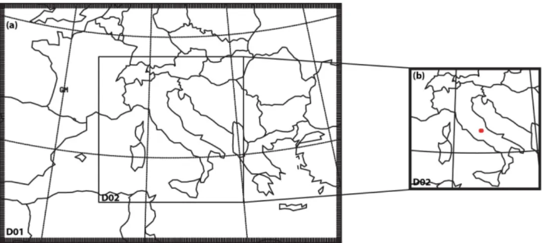
Figure 4. Model configuration for WRF simulations using two domains: (a)overlapping of 12 and 3 km;(b) the high-resolution D02 (1x=3 km) includes the Monte Midia radar (red dot in the figure).
−40 −30 −20 −10 0 10 20 30 40
100
200
300
400
500
600
700
800
900
1000 2 m 0.4 1 2 4 7 10 16 24 32 40g/kg 661 m
1366 m 2945 m 5550 m 7190 m 9180 m 10370 m 11810 m 13680 m
SLAT 41.65 SLON 12.43 SELV 32.00 SHOW 0.58 LIFT −0.05 LFTV −0.12 SWET 176.2 KINX 33.00 CTOT 25.10 VTOT 25.50 TOTL 50.60 CAPE 47.73 CAPV 57.86 CINS −9.31 CINV −7.90 EQLV 442.3 EQTV 442.2 LFCT 866.5 LFCV 870.6 BRCH 1.47 BRCV 1.78 LCLT 285.8 LCLP 947.1 MLTH 290.3 MLMR 9.85 THCK 5548. PWAT 31.15
00Z 20 May 2008 University of Wyoming 16245 LIRE Pratica Di Mare
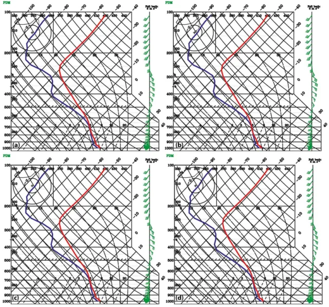
Figure 5.PDM sounding at 00:00 UTC, 20 May 2008.
wherexbis the generic variable of an a priori state (first guess),yois the observation, andHis the operator that con-verts the model state to the observation space. This cost func-tion J measures the distance of a field x from the obser-vationsyoand from the backgroundxb: these distances are scaled through the matricesRandB, the observation and the background error covariance matrices, respectively. A cor-rect evaluation of the error covariance matrices, bothBand R, is crucial to a good-quality final analysis. The observa-tion covariance error matrix Ris usually diagonal, because the correlations between different instruments are assumed
2924 I. Maiello et al.: Impact of radar data assimilation using WRF-3DVAR
Figure 6.WRF sounding at 00:00 UTC on 20 May 2008 at PDM for(a)CTL,(b)CON,(c)RAD, and(d)ALL.
averages differences, valid at the same timet0, between two
forecasts, one of them starting several hours later than the other (e.g., month-long series of 24 h minus 12 h forecasts valid at the same time). The only requirement is that the time t0is large enough to avoid any problem related to the model
spin-up. A detailed description of the 3DVAR system can be found in Barker et al. (2003, 2004).
3.2 Radar data assimilation methodology
Doppler radar data contain important high-resolution mete-orological features. Radial velocity produces information on the atmospheric motions that is important for the onset of convection; moreover, it is well known that radar reflectivity is a measurement of the amount of precipitating hydrome-teors (rain, snow, etc.). However, due to the complexity of coding, such variables are not included in most of the data assimilation schemes.
On the contrary, the WRF–3DVAR operator for the assim-ilation of Doppler radar data accounts for both reflectivity and the vertical velocity component of radial velocity. Ver-tical increments are estimated, including a balance equation based on Richardson (1922). This is the so-called linearized Richardson equation, which combines a continuity equation, an adiabatic thermodynamic equation, and a hydrostatic re-lation: it becomes important when radar data are included in the analysis.
Moreover, the total waterqt is used as the moisture
Figure 7. (a)VMI (dBZ) from the Monte Midia radar at 14:00 UTC, 20 May 2008 (courtesy of Centro Funzionale of the Abruzzo region). The solid red circle and the red arrow indicate the precipitation patterns selected for the analysis.(b) Geostationary MSG map taken at 14:00 UTC at the visible channel.(c)Geostationary MSG map taken at 14:00 UTC at the infrared channel. The “banana-shaped” cloud structure is clearly evident over the central Tyrrhenian Sea.
Data from the Monte Midia radar (42◦03′28′′N, 13◦10′38′′E) are provided by the Centro Funzionale of the Abruzzo region, and they are assimilated to improve high-resolution initial conditions. The Monte Midia radar is a C-band Doppler radar located on the border between the Abruzzo and Lazio regions. It is part of the national radar mosaic, and it is placed at 1710 m above the sea level (1660 m plus a tower of 50 m). It covers most of central Italy, including the Abruzzo interior and the urban area of Rome, as shown in Fig. 3. Reflectivity and radial velocity are detected every 15 and 30 min, respectively, at a 500 m horizontal resolution with four antenna elevation angles (0, 1, 2, and 3◦).
It is well known that radar observations can be affected by several sources of errors, mainly due to ground clutter, at-tenuation and radio interferences. Particularly, weather radar operating in complex orography may be affected by a signif-icant beam blockage that can strongly degrade the monitor-ing capabilities and accordmonitor-ingly the rainfall estimation at the ground.
2926 I. Maiello et al.: Impact of radar data assimilation using WRF-3DVAR
Figure 8.WRF reflectivity (dBZ) at 14:00 UTC on 20 May 2008 for experiments(a)CTL,(b)CON,(c)RAD and(d)ALL.
Figure 9.12 h accumulated rainfall between 10:00 and 22:00 UTC on 20 May 2008 estimated by the Monte Midia radar.
filter. Partial beam blockage is corrected by adopting a com-pensating technique (Fulton et al., 1998), while attenuation is mitigated by means of rain path-integrated attenuation (PIA) techniques (Picciotti et al., 2006). Once corrected, both reflectivity and velocity data are ready for ingestion into 3DVAR. Typical errors of 5.0 m s−1 for radial velocity and 5.0 dBZ for reflectivity are assumed. The assimilation window has been set to±5 min at the analysis time. Finally,
a total number of 344 160 radar observations were ingested into the model.
3.3 Radar observation operators: radial velocity and reflectivity
To assimilate radar observations, the following observation terms are added to the existing cost function:
J=Jold+
1 2
Xk
k=0
h
Vrk−VrkoTRv−1 Vrk−Vrko
+1
2 Zk−Z
o
k
T
R−z1 Zk−Zok
, (2)
where Jold is used to represent the existing cost function
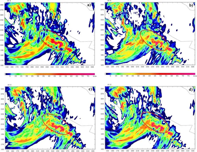
Figure 10.12 h accumulated rainfall ending at 22:00 UTC on 20 May 2008 estimated by WRF experiments:(a)CTL,(b)CON,(c)RAD and(d)ALL.
Vr stand for the radial velocity and Z for the reflectivity
factor. The superscript “o” indicates the observations. The symbols R−1
v andR−z1 stand for observation error covari-ance matrices for radial velocity and reflectivity, respectively (Sun and Wang, 2013). Note that the summation over the ob-servation time levelskis not needed in the case of 3DVAR. As explained previously, the observation operatorH in the cost function (1) links the model variables in a model coordi-nate to the observation variables in an observation space. For the radar radial velocity, this linkage is formulated with the three-dimensional wind field (u,v, andw), the hydrometeor fall speed or terminal velocityvt, and the distancerbetween
the location of a data point and the radar antenna: Vr=u
x−xi ri
+vy−yi ri
+(w−vt)
z−zi ri
, (3)
where (x, y, z) represents the location of the observation point and (xi, yi, zi)represents the location of the radar sta-tion.
Following the algorithm of Sun and Crook (1998), the ter-minal velocity is given by
vt=5.40a·qr0.125, (4)
where “a” is a correction factor defined as follows: a= p0p¯
0.4
, (5)
wherep¯is the base-state pressure andp0is the pressure at
the ground.
The formulation of the reflectivity operator is not as straightforward, because it depends on the assumption of drop size distribution in a microphysical parameterization scheme and the classification of hydrometeors. To assimi-late radar reflectivity directly, the total water mixing ratioqt
was chosen as a control variable, and a warm rain process was introduced (Dudhia, 1989) into the WRF–3DVAR sys-tem. This allowed the increments of moist variables linked to the hydrometeors to be produced, such as the water vapor mixing ratioqv, the cloud water mixing ratioqc, and the
rain-water mixing ratioqr. Once the 3DVAR system produces the
qc andqr increments, the setup of the observation operator
for the assimilation of reflectivity is obtained.
Following Sun and Crook (1997), Xiao et al. (2007) used the following relation for WRF–3DVAR:
2928 I. Maiello et al.: Impact of radar data assimilation using WRF-3DVAR
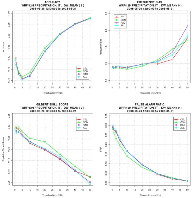
Figure 11.ACC (top left), FBIAS (top right), ETS (bottom left) and FAR (bottom right) as a function of threshold. The red line shows CTL, the green line CON, the violet line RAD, and the cyan line ALL.
whereZ is the radar reflectivity expressed in dBZ,ρ is the air density (kg m−3) and qr is the rain water mixing
ra-tio (g kg−1). This relation was derived analytically by assum-ing a Marshall–Palmer distribution of raindrop size with in-terceptN0=8×106mm−4, and no contribution of ice phases
to the reflectivity is accounted for.
Equation (6) was used in cost function (2) to assimilate re-flectivity in the WRF–3VAR developed by Xiao et al. (2007).
4 Experimental setup 4.1 Model setup
WRF model version 3.4.1 (Wang et al., 2011) is used for this study. Two domains (D0i), running independently, are used (Fig. 4). The outer domain (D01) has a resolution of 12 km with a number of horizontal grid points of 263×185.
It is initialized using ECMWF analysis, and the boundary conditions are upgraded every 6 h. The inner domain (D02) has a horizontal grid spacing of 3 km (445×449), and it is
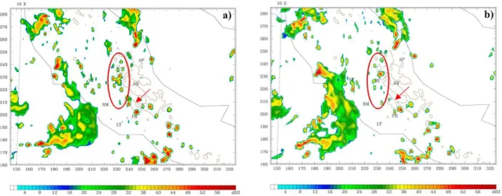
Figure 12.Reflectivity (dBZ) simulated by the ALL_2OL(a)and ALL_3OL(b)experiments with two and three outer loops, respectively, at 14:00 UTC, 20 May 2008.
The new Thompson et al. scheme (Thompson et al., 2008) for microphysics, the Kain–Fritsch scheme (Kain, 2004) for cumulus convection, for D01 only, the Mellor, Yamada, Nakanishi and Niino level 2.5 (Nakanishi and Niino, 2006) for planetary boundary layers, the rapid radiative transfer model (Mlawer et al., 1997) and the Goddard (Chou and Suarez, 1994) schemes for longwave and shortwave radia-tion, respectively, are used for all the experiments. The Noah land surface model (LSM; the successor to the OSU (Oregon State University) LSM described by Chen and Dudhia, 2001) for land surfaces is used.
Besides the first guess xb and the observations yo, as explained in Sect. 3.1, another important input for WRF– 3DVAR is the background error covariance matrixB. This is computed using the NMC method, and a domain-specificB has been generated (CV5 option) using the empirical orthog-onal function (EOF) to represent the vertical covariance.
To estimate the NMC-based error statistics, two forecasts have been performed every day for a period of 1 week (Sug-imoto et al., 2009) starting on 15 May 2008: a 24 h fore-cast (starting at 00:00 UTC) and a 12 h forefore-cast (starting at 12:00 UTC) valid at the same time. The differences between the two forecasts att+24 andt+12 are used to calculate the domain-averaged error statistics.
4.2 Experimental design
Several experiments are performed with the aim of improv-ing ICs. The GTS (Global Telecommunication System) con-ventional observations – SYNOP (surface synoptic obser-vations) and TEMP (upper-level temperature, humidity and winds) – are used with and without non-conventional radar data. The assimilation window for conventional data is set to ±1 h, whereas the one for radar data is set to ±5 min
at the analysis time. To verify the impact of radar data, a
total of four WRF experiments are performed for the high-resolution domain (3 km): in the control experiment (CTL), no data assimilation is performed; in the CON experiment, the assimilation of SYNOP and TEMP observations is per-formed at 00:00 UTC, 20 May 2008; in the RAD experi-ment, the assimilation of Monte Midia radar data (both re-flectivity and radial velocity) is performed; in the ALL ex-periment, both conventional data (SYNOP and TEMP) and radar data are ingested. A specific background error covari-ance matrix calculated for the highest-resolution domain is used for CON, RAD and ALL. For these above simulations, one outer loop is used as the default. Two additional exper-iments (ALL_2OL and ALL_3OL) are carried out similarly to ALL, but using two and three outer loops, respectively, during the assimilation procedure. The multiple outer loop strategy (Rizvi et al., 2008) allows for the inclusion of non-linearity in the observation operators and for the assessment of the influence of observations entering for each cycle. The non-linear problem is solved iteratively as a sequence of lin-ear problems by running more than one analysis outer loop, so the assimilation system is able to ingest more observa-tions.
All experiments last 24 h, from 00:00 UTC, 20 May 2008 until 00:00 UTC, 21 May. They are summarized in Table 1.
5 Results
5.1 Initial conditions
2930 I. Maiello et al.: Impact of radar data assimilation using WRF-3DVAR
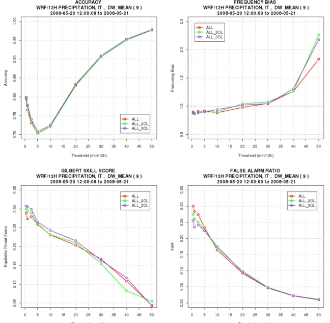
Figure 13.Outer loop sensitivity: ACC, FBIAS, ETS and FAR for ALL, ALL_2OL and ALL_3OL. The red line refers to one loop, the green line to two loops, and the violet line to three loops.
available potential energy (CAPE), useful for assessing the instability of the atmosphere and therefore the possibility of triggering convection, a lifted index (LI), which measures the severity of the thunderstorm, and theK index, which gives an indication of the thunderstorm occurrence. The CAPE at Pratica di Mare suggests a weakly unstable environment and that severe thunderstorms are unlikely to occur (small LI). No significant differences are found between the experiments, except for the LI listed in Table 2. The CAPE is significantly underestimated for all simulations, whereas the LI is overes-timated. The WRF K index is in good agreement with the observed one.
The observed and WRF radio soundings at Pratica Di Mare at 00:00 UTC, 20 May 2008 (Figs. 5 and 6, respec-tively) clearly show no large differences between the WRF
20 May 2008) and location (41◦65′N, 12◦43′E).
Index PDM CTL CON RAD ALL CAPE (J Kg−1) 47.7 0 0 0 0 LI (◦C) −0.1 0.6 1.2 0.6 0.6
K(◦C) 33 32 32 32 32
5.2 Impact on radar reflectivity and rainfall
The impact of Monte Midia radar data assimilation on the forecast is evaluated by comparing the observed reflectivity and the estimated rain rate with those produced by the WRF experiments.
5.2.1 Impact on the precipitation forecast
The VMI (vertical maximum intensity) reflectivity of the Monte Midia radar at 14:00 UTC on 20 May clearly shows the precipitation in central Italy (Fig. 7a) and on the seaside near the Lazio coast. Precipitation can also be inferred from the cloudiness derived from the Geostationary MSG (Me-teosat Second Generation) satellite images (Fig. 7b, c), where a “banana-shaped” cloud structure is also clearly shown over the central Tyrrhenian Sea. Aligned cells are also detected inland near Rieti (Fig. 7a, red circle). The Monte Midia radar highlights this last feature: a reflectivity of approximately 50–55 dBZ at 14:00 UTC associated with a few small con-vective cells oriented north–south between Rome (RM) and Rieti (RI) (solid red oval in Fig. 7a) is clearly detected by the radar. Another area of moderate precipitation (about 40 dBZ on the border between Lazio and Abruzzo) was also detected (red arrow in Fig. 7a).
The CTL simulation clearly shows (Fig. 8a) a large area of reflectivity over the sea that is overestimated both in amount and the affected area. Moreover, an attempt to reproduce the small convective cells between Rome and Rieti is also found, but these small cells are wrongly oriented and the reflectiv-ity is underestimated. The assimilation of conventional data (Fig. 8b) removes part of the north–south oriented area of reflectivity north of Viterbo (VT), making it closer to the
of the area covered by the cells near Rieti, but they are not yet correctly aligned. The RAD simulation (Fig. 8c) partly reduces the areal distribution of the reflectivity over the sea-side, showing an attempt to separate the two elongated areas of reflectivity as they can be deduced by the satellite image (Fig. 7b, c). Moreover, RAD both reduces the convection in the Viterbo area and correctly generates aligned cells north of Rome near Rieti (Fig. 8c, red oval), as the Monte Midia radar detected (Fig. 7a). The assimilation of radar and conventional data (ALL, Fig. 8d) shows a distribution of the reflectivity over the Tyrrhenian Sea even closer to the one deduced by the satellite images than by RAD, but an over-reduction of the structure and reflectivity of the cells north of Rieti is also found. The previous analysis suggests that the assimilation of radar reflectivity and radial velocity largely impacts the forecast even if only one radar is assimilated. Moreover, the assimilation of either the radar data only or the radar and convectional data together reduces the differences between the forecast and the observation.
Similar to the reflectivity, a comparison between the ob-served (Fig. 9) and the WRF 12 h accumulated rainfall (Fig. 10) is now performed.
2932 I. Maiello et al.: Impact of radar data assimilation using WRF-3DVAR
are found for the precipitation inland between CTL, CON and RAD. This last one is the sole simulation able to pro-duce a red spot in the Rieti area (Fig. 10c) like the observed one (Fig. 9) clearly related to the aligned cells discussed pre-viously. Similarly to CTL and CON, ALL (Fig. 10d) does not produce the red spot of precipitation in the Rieti area, but the precipitation between RM and FR is correctly reproduced, as for CTL and RAD.
In summary, the precipitation forecast also clearly shows an impact of the radar data assimilation by producing a pre-cipitation pattern closer to the observed one.
5.3 Statistical evaluation
In order to compare the experiments carried out for the Aniene event objectively, four statistical indicators are used (Wilks, 1995): forecast accuracy (ACC), false alarm rate (FAR), frequency bias (FBIAS) and equitable threat score (ETS).
The ACC index shows the accuracy of the forecast; a per-fect forecast has ACC=1. FAR estimates the forecast
fre-quency failures; a perfect forecast has FAR=0. FBIAS gives
information on the correctness of a precipitation forecast: values greater than 1 indicate an overestimation in the num-ber of forecast events; the perfect value is FBIAS=1. ETS
represents the fraction of the events reproduced correctly, taking into account random hit chance; the best value is 1. The ETS index may have values lower than or near zero if the forecasts are wrong, so values of 0.5/0.6 are fairly good. Figure 11 shows the results for the previous indexes for the 12 h accumulated rainfall as a function of different thresh-olds. The WRF simulations show no large differences be-tween them, but ACC clearly shows improvements for CON (Fig. 11, green line) with respect to other experiments for thresholds between 5 and 30 mm/12 h; accordingly, the FAR index for CON shows values lower than the others for the same thresholds. Moreover, CON produces the best values for ETS at all thresholds, even though it rapidly degrades for the higher ones. Vice versa, FBIAS gives the worst values for CON between 5 and 20 mm/12 h, whereas it improves for higher thresholds between 30 and 40 mm/12 h. More-over, the values of FBIAS are close to the best value of 1 for thresholds lower than 30 mm/12 h for all the simulations, whereas this index has values greater than 1 for all the exper-iments.
These results do not support completely the previous find-ing that the RAD and ALL experiments produce a better forecast; this disagreement is probably produced by the rain gauge location. In fact, the highest density of surface stations is nearby Rome (Fig. 3), where the CON simulation produces rainfall in good agreement with the observation.
6 Impact of outer loops on precipitation
Based on the previous results, a set of sensitivity tests for WRF–3DVAR is performed for the ALL experiment only. These new experiments are carried out using two and three outer loops during the assimilation procedure (Table 3). All the experiments performed using 3DVAR (CON, RAD and ALL) discussed previously are carried out using one outer loop. The multiple outer loop strategy (Rizvi et al., 2008) allows for the inclusion of non-linearity in the observation operators and for the assessment of the influence of obser-vations entering for each cycle. The non-linear problem is solved iteratively as a sequence of linear problems by run-ning more than one analysis outer loop, so the assimilation system is able to ingest more observations.
As already pointed out in Sect. 5.2.1, ALL (Fig. 8d) pro-duces a reduction in the differences between the forecast and the observed reflectivity. Using two outer loops during the assimilation procedure, a strong areal attenuation of the dBZ over Viterbo is obtained (Fig. 12a), but at the same time, the aligned cells near Rieti are not reproduced exactly. Adding one more loop (ALL_3OL, Fig. 12b), the reflectivity near Viterbo is increased again, whereas the cells north of Rieti are reproduced better: they are similar to what ALL produces and to what the Monte Midia radar detected. Finally, the “banana-shaped” structure over the central Tyrrhenian Sea is well defined. These results suggest that the increase in the number of outer loops may positively impact the forecast for heavy rainfall.
To evaluate the impact of outer loops better, ACC, FAR, FBIAS and ETS are used again. From the ACC index graph, no large differences are highlighted between the three exper-iments. On the other hand, FBIAS shows small differences for thresholds between 10 and 30 mm/12 h for ALL_2OL and ALL_3OL (Fig. 13, upper right, green and violet curves, respectively): both have values close to 1. The ETS index produces better scores for ALL_3OL (violet curve, Fig. 13, bottom left) for thresholds lower than 30 mm/12 h. Finally, FAR gives a quite good response for the two experiments if using more than one outer loop (green and violet curves, Fig. 13, bottom right) for very low thresholds between 0 and 5 mm/12 h.
The previous results confirm that the increase in the num-ber of outer loops may positively impact the forecast for heavy rainfall.
7 Summary and conclusions
gether with conventional observations (ALL). If using more than one outer loop, for the ALL experiment only, a positive impact is obtained for two and three outer loops (ALL_2OL and ALL_3OL, respectively). Statistical indicators are used to compare the model simulations objectively. The statistical results do not support the previous finding, mostly because the surface stations are concentrated near the urban area of Rome. Obviously, the assimilation of these stations (CON) drives the results toward them. Statistical indicators are also used to investigate the outer loop impact: in this case, statis-tics confirm the model results. This is because the multiple outer loop technique allows the assimilation of a larger num-ber of observations progressively into WRF–3DVAR.
In conclusion, the assimilation of radar radial velocity and reflectivity data shows a positive impact on precipitation forecasts, also if they are ingested together with conventional observations and if the outer loop strategy is used.
Finally, to evaluate the previous results properly, it has also to be considered that the WRF–3DVAR radar data assimila-tion scheme has a few limitaassimila-tions:
1. the lack of the ice phase in the 3DVAR microphysics; 2. the estimation of theBmatrix for high-resolution data
assimilation can be improved by using the ensemble ap-proach or by the combined use of an ensemble Kalman filter.
Moreover, the lack of radar coverage on the Tyrrhenian coast-line from where the system approaches it is also a limiting factor in the assimilation process.
Finally, the technique of multiple outer loops will be inves-tigated further by tuning length-scale and observation error parameters, and thinning of radar data has to be undertaken either to reduce the observation-error spatial correlation or the computational cost of the assimilation (Montmerle and Faccani, 2009). Moreover, following Wang et al. (2013), the new observation operator that, instead of assimilating radar reflectivity directly, assimilates retrieved rainwater and wa-ter vapor derived from radar reflectivity, could be applied. Wang et al. (2013) showed that one of the problems of as-similating the reflectivity is in the use of a linearizedZ−qr
(reflectivity–rainwater) equation as the observation operator
well as using data from several operative radars located in central Italy, also including dual-polarization systems.
Acknowledgements. The authors are grateful to HIMET (High Innovation in Meteorology and Environmental Technologies) and Sapienza University of Rome for radar and computing resources support, as well as the National Department for Civil Protection. NCAR is also acknowledged for the WRF and 3DVAR systems.
Edited by: G. Pappalardo
References
Barker, D. M., Huang, W., Guo, Y.-G., and Bourgeois, A.: A Three-Dimensional Variational (3DVAR) Data Assimilation System For Use With MM5, NCAR Tech. Note, NCAR/TN-453+STR, UCAR Communications, Boulder, CO, 68 pp., 2003.
Barker, D. M., Huang, W., Guo, Y.-R., Bourgeois, A., and Xiao, Q.: A Three-Dimensional Variational (3DVAR) Data Assimila-tion System For Use With MM5: ImplementaAssimila-tion and Initial Re-sults, Mon. Weather Rev., 132, 897–914, 2004.
Bech, J., Codina, B., Lorente, J., and Bebbington, D.: The sensitiv-ity of single polarization weather radar beam blockage correc-tion to variability in the vertical refractivity gradient, J. Atmos. Oceanic Technol., 20, 845–855, 2003.
Chen, F. and Dudhia, J.: Coupling an advanced land-surface/hydrology model with the Penn State/NCAR MM5 modeling system. Part I: Model description and implementation, Mon. Weather Rev., 129, 569–585, 2001
Chou M.-D. and Suarez, M. J.: An efficient thermal infrared ra-diation parameterization for use in general circulation models, NASA Tech. Memo, 104606, 3, 85 pp., 1994.
Courtier, P., Thépaut, J.-N., and Hollingsworth, A.: A strategy for operational implementation of 4D-Var using an incremental ap-proach, Q. J. Roy Meteorol. Soc., 120, 1367–1387, 1994. Dudhia, J.: Numerical Study of Convection Observed during
the Winter Monsoon Experiment Using a Mesoscale Two-Dimensionale Model, J. Atmos. Sci., 46, 3077–3107, 1989. Fisher, M.: Background Error Statistics derived from en ensemble
2934 I. Maiello et al.: Impact of radar data assimilation using WRF-3DVAR
Fulton, R. A., Breidenbach, J. P., Seo, D., Miller, D., and O’Bannon, T.: The WSR-88D rainfall algorithm, Weather Forecast., 13, 377–395, 1998.
Gao, J., Xue, M., Brewster, K., and Droegemeier, K. K.: A three dimensional variational data analysis method with recursive filter for Doppler radars, J. Atmos. Oceanic Technol., 21, 457–469, 2004.
Kain, J. S.: The Kain-Fritsch convective parameterization: an up-date, J. Appl. Meteor., 43, 170–181, 2004.
Kalnay, E.: Atmospheric modeling, data assimilation and pre-dictability, Cambridge University Press, Cambridge, UK, 364 pp., 2003.
Lindskog, M., Salonen, K., Jarvinen, H., and Michelson, D. B.: Doppler Radar Wind Data Assimilation with HIRLAM 3DVAR, Am. Meteorol. Soc., 132, 1081–1092, 2004.
Mlawer, E. J., Taubman, S. J., Brown, P. D., Iacono, M. J., and Clough, S. A.: Radiative transfer for inhomogeneous atmo-sphere: RRTM, a validated correlated-k model for the long-wave, J. Jeophys. Res., 102, 16663–16682, 1997.
Montmerle, T. and Faccani, C.: Mesoscale assimilation of radial velocities from Doppler radars in a preoperational framework, Mon. Weather Rev., 137, 1939–1953, 2009.
Nakanishi, M. and Niino, H.: An Improved Mellor–Yamada Level-3 Model: Its Numerical Stability and Application to a Regional Prediction of Advection Fog, Bound.-Layer Meteorol., 119, 397– 407, 2006.
Parrish, D. F. and Derber, J. C.: The National Meteorological Cen-ter’s Spectral Statistical-Interpolation Analysis System, Mon. Weather Rev., 120, 1747–1763, 1992.
Picciotti, E., Montopoli, M., Gallese, B., Cimoroni, A., Ferrauto, G., Ronzitti, L., Mancini, G., Volpi, A., Sabatini, F., Bernardini, L., and Marzano, F. S.: Rainfall mapping in complex orography from C-band RADAR at Mt. Midia in Central Italy: data synergy and adaptive algorithms, Proceeding of ERAD 2006, Barcelona, Spain, 341–344, 2006.
Picciotti, E., Montopoli, M., Di Fabio, S., and Marzano, F. S.: Statis-tical Calibration of Surface Rain Fields from C-band Mt. Midia Operational RADAR in Central Italy, ERAD 2010, Sibiu, Roma-nia, 2010.
Richardson, L. F.: Weather prediction by numerical process, Cam-bridge University Press, CamCam-bridge, UK, 236 pp., 1922. Rizvi, S., Guo, Y.-R., Shao, H., Demirtas, M., and Huang,
X.-Y.: Impact of outer loop for WRF data assimilation system (WRFDA), 9th WRF Users’ Workshop, Boulder, Colorado, 23– 27 June 2008.
Skamarock, W. C., Klemp, J. B., Dudhia, J., Gill, D. O., Barker, D. M., Duda, M. G., Huang, X.-Y., Wang, W., and Powers, J. G.: A description of the Advanced Reasearch WRF Version 3. NCAR Technical Note, TN 475+STR, 113 pp., available at: www.mmm.ucar.edu/wrf/users/docs/arwv3.pdf (last access: Jan-uary 2012), 2008.
Sugimoto, S., Crook, N. A., Sun, J., Xiao, Q., and Barker, D. M.: An examination of WRF 3DVAR radar data assimilation on its capa-bility in retrieving unobserved variables and forecasting precip-itation through observing system simulation experiments, Mon. Weather Rev., 137, 4011–4029, doi:10.1175/2009MWR2839.1, 2009.
Sun, J. and Crook, N. A.: Dynamical and Microphysical Retrieval from Doppler RADAR Observations Using a Cloud Model and
Its Adjoint, Part I: Model Development and Simulated Data Ex-periments, J. Atmos. Sci., 54, 1642–1661, 1997.
Sun, J. and Crook, N. A.: Dynamical and Microphysical Retrieval from Doppler RADAR Observations Using a Cloud Model and Its Adjoint, Part II: Retrieval Experiments of an Observed Florida Convective Storm, J. Atmos. Sci., 55, 835–852, 1998.
Sun, J. and Wang, H.: Radar data assimilation with WRF 4DVar. Part II: comparison with 3D-Var for a squall line over the US Great Plains, Mon. Weather Rev., 11, 2245–2264, doi:10.1175/MWR-D-12-00169.1, 2012.
Sun, J. and Wang, H.: WRF-ARW variational storm-scale data as-similation: current capabilities and future developments, Adv. Meteorol., 2013, 815910, doi:10.1155/2013/815910, 2013. Sun, J., Flicker, D. W., and Lilly, D. K.: Recovery of three
di-mensional wind and temperature fields from simulated single-Doppler radar data, J. Atmos. Sci., 48, 876–890, 1991.
Sun, J., Chen, M., and Wang, Y.: A frequent-updating analysis sys-tem based on radar, surface, and mesoscale model data for the Beijing 2008 forecast demonstration project, Weather Forecast, 25, 1715–1735, 2010.
Thompson G., Field, R., Rasmussen, R. M., and Hall, W. D.: Ex-plicit forecasts of winter precipitation using an improved bulk microphysics scheme, Part II: implementation of a new snow pa-rameterization, Am. Meteorol. Soc., 136, 5095–5115, 2008. Vulpiani, G., Pagliara, P., Negri, M., Rossi, L., Gioia, A., Giordano,
P., Alberoni, P. P., Cremonini, R., Ferraris, L., and Marzano, F. S.: The Italian radar network within the national early-warning sys-tem for multi-risks management, Proc. of Fifth European Con-ference on Radar in Meteorology and Hydrology (ERAD 2008), 184, Finnish Meteorological Institute, Helsinki, 30 June–4 July, 2008.
Wang, H., Sun, J., Zhang, X., Huang, X., and Auligne, T.: Radar data assimilation with WRF 4D-Var. Part I: system development and preliminary testing, Mon. Weather Rev., 141, 2224–2244, 2013.
Wang, H., Sun, J., Fan, S., and Huang, X. Y.: Indirect assimilation of radar reflectivity with WRF 3D-Var and its impact on pre-diction of four summertime convective events, J. Appl. Meteor. Climatol., 52, 889–902, 2013.
Wang, W., Bruyère, C., Duda, M., Dudhia, J., Gill, D., Lin, H.-C., Michalakes, J., Rizvi S., and Zhang X., Beezley J. D., Coen J. L., and Mandel J.: ARW, Version 3 Modeling Sys-tem User’s Guide, Mesoscale and Microscale Meteorology Di-vision, National Center for Atmospheric Research, 2011, avail-able at: http://www.mmm.ucar.edu/wrf/users/docs/user_guide_ V3/ARWUsersGuideV3.pdf (last access: April 2011), 2011. Wilks, D. S.: Statistical Methods in the Atmospheric Sciences,
Aca-demic Press, San Diego, USA, 467 pp., 1995.
Xiao, Q. and Sun, J.: Multiple-RADAR Data Assimilation and Short-Range Quantitative Precipitation Forecasting of a Squall Line Observed during IHOP_2002, Mon. Weather Rev., 135, 3381–3404, 2007.
Xiao, Q., Kuo, Y.-H., Sun, J., and Lee, W.-C.: Assimilation of Doppler RADAR Observations with a Regional 3DVAR System: Impact of Doppler Velocities on Forecasts of a Heavy Rainfall Case, J. Appl. Meteor., 44, 768–788, 2005.