www.hydrol-earth-syst-sci.net/21/267/2017/ doi:10.5194/hess-21-267-2017
© Author(s) 2017. CC Attribution 3.0 License.
Improving the precipitation accumulation analysis using lightning
measurements and different integration periods
Erik Gregow1, Antti Pessi2, Antti Mäkelä1, and Elena Saltikoff1
1Meteorological Research, Finnish Meteorological Institute, P.O. Box 503, 00101 Helsinki, Finland 2Applied Meteorology, Vaisala, 3 Lan Dr., Westford, MA 01886, USA
Correspondence to:Erik Gregow ([email protected])
Received: 7 March 2016 – Published in Hydrol. Earth Syst. Sci. Discuss.: 17 March 2016 Revised: 24 November 2016 – Accepted: 17 December 2016 – Published: 11 January 2017
Abstract. The focus of this article is to improve the pre-cipitation accumulation analysis, with special focus on the intense precipitation events. Two main objectives are ad-dressed: (i) the assimilation of lightning observations to-gether with radar and gauge measurements, and (ii) the anal-ysis of the impact of different integration periods in the radar–gauge correction method. The article is a continuation of previous work by Gregow et al. (2013) in the same re-search field.
A new lightning data assimilation method has been im-plemented and validated within the Finnish Meteorological Institute – Local Analysis and Prediction System. Lightning data do improve the analysis when no radars are available, and even with radar data, lightning data have a positive im-pact on the results.
The radar–gauge assimilation method is highly dependent on statistical relationships between radar and gauges, when performing the correction to the precipitation accumulation field. Here, we investigate the usage of different time inte-gration intervals: 1, 6, 12, 24 h and 7 days. This will change the amount of data used and affect the statistical calculation of the radar–gauge relations. Verification shows that the real-time analysis using the 1 h integration real-time length gives the best results.
1 Introduction
Accurate estimates of accumulated precipitation are needed for several applications such as flood protection, hydropower, road- and fire-weather models. In Finland, one of the most economically relevant users of precipitation is the
hy-dropower industry. Between 10 and 20 % of Finnish annual electric power production comes from hydropower, depend-ing on the amount of precipitation and water levels in dams and water reservoirs. In order to maintain correct calcula-tion of the energy supplied to customers and to avoid (or at least minimize) the environmental risks and economical losses during extreme precipitation and flooding events, a profound analysis of the expected water amounts in dams and reservoirs from catchment areas is needed. The current hydropower strategy of Finland is to increase capacity by improving the efficiency of existing plants through techni-cal adjustments. The maintenance and planning of proper dam structures need the most up-to-date information about the rain rates to be able to adjust the regulation functions of the dams, both for the current and the changing climatic con-ditions (IPCC-AR5, 2013).
interrup-situations. In their study, the nonparametric kriging with ex-ternal drift outperformed other methods in an accumulation period of 60 min. Wang et al. (2015) developed a sophisti-cated method for urban hydrology, which preserves the non-normal characteristics of the precipitation field. They also noticed that common methods have a tendency to smooth out the important but spatially limited extremes of precipitation. Comparing radars and gauges, an additional challenge arises from the different sampling sizes of the instruments. Radar measurement volume can be several kilometers wide and thick (a 1◦
beam is approximately 5 km wide at 250 km), while the measurement area of a gauge is 400 cm2 (weigh-ing gauges) or 100 cm3(optical instruments). Part of the dis-parateness of radar and gauge measurements is due to vari-ability of the raindrop size distribution within the area of a single radar pixel. Jaffrain and Berne (2012) have observed variability up to 15 % of the rain rate in a 1×1 km pixel, with time steps of 1 min.
Lightning is associated with convective precipitation, but in areas where a large portion of precipitation is stratiform, lightning data alone are not adequate for precipitation esti-mation. Although convective events contribute only a frac-tion of the annual precipitafrac-tion amount, they might be im-portant during flooding events. However, lightning has been used to complement and improve other datasets. Morales and Agnastou (2003) combined lightning with satellite-based measurements to distinguish between convective and strat-iform precipitation area and achieved a remarkable 31 % bias reduction, compared to satellite-only techniques. Light-ning has also been assimilated to numerical weather predic-tion (NWP) models, using nudging techniques, or improv-ing the initialization process of the model. This can be done by blending them with other remote sensing data to create heating profiles (e.g., estimating the latent heat release when precipitation is condensed). Papadopulos et al. (2005) used lightning data to identify convective areas and then modified the model humidity profiles, allowing the model to produce convection and release latent heat using its own convective parameterization scheme. They combined lightning with 6-hourly gauge data, within a mesoscale model in the Mediter-ranean area, and showed improvement in forecasts up to 12 h lead time. Pessi and Businger (2009) derived a lightning–
backup plan in the occasions when radar data are either miss-ing or of deteriorated quality. Even though these occasions are rare, they often occur on days when detailed precipita-tion estimates are of great interest. Thunderstorms produc-ing heavy localized rainfall are also often producproduc-ing heavy winds, causing unavailability of radar data due to breaks on electricity and data communications. Our principal goal is to have as good an analysis as possible, which is different from having a best analysis to start a model.
Gregow et al. (2013) have demonstrated the benefit of assimilating different data sources (radars and gauges) in precipitation estimation. The largest uncertainties were ob-served during heavy convective rainfall. These are the situ-ations when lightning occurs. The accumulation process is based on the radar reflectivity field, where gauges correct the initial field; e.g., if there is no reflectivity field, there is no accumulation (gauges are not used alone). To improve the spatially accurate real-time precipitation analysis, new meth-ods are adopted by fusion of weather radar, lightning obser-vations and rain gauge information in novel ways. This leads to better possibilities in estimating convective rainfall events (i.e., > 5 mm h−1) and the accumulated precipitation for the benefit of hydropower management and other related appli-cation areas. The work reported here has been performed us-ing the Local Analysis and Prediction System (LAPS), which is used operationally in the weather service of the Finnish Meteorological Institute (FMI). Testing new approaches in an operational system has its challenges. For example, it is not possible to exclude a large amount of independent refer-ence stations. Also, the possibilities to rerun cases with dif-ferent settings have been limited. The major benefit of work-ing in an operational environment is that we can be sure that we only use data and methods which are operationally avail-able and feasible.
2 Observations and instrumentation
Here, we describe the three data sources employed in this study (rain gauge, radar and lightning observations) and the verification periods used in this study.
2.1 Rain gauge observations
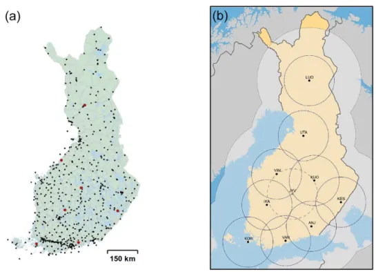
Rain gauges provide point observations of the accumula-tion. They are usually considered more accurate than radar as point values and are frequently used to correct the radar field (Wilson and Brandes, 1979). The surface precipitation network (in total, 472 stations) consists of standard weight-ing gauges and optical sensors mounted on road-weather masts. Since 2015, FMI has managed 102 stations instru-mented with the weighting gauge OTT Messtechnik Plu-vio2. The Finnish Transport Agency (FTA) runs 370 road-weather stations with optical sensor measurements (Vaisala Present Weather Detectors models PWD22 and, to some ex-tent, PWD11). The precipitation intensity is measured in dif-ferent time intervals which are summed up to 1 h precipita-tion accumulaprecipita-tion informaprecipita-tion. Uncertainties and more de-tailed information can be found in Gregow et al. (2013). If measurements consistently indicate poor data quality, either manually identified from station error logs or by inspecting the data, those stations are blacklisted within the LAPS pro-cess and do not contribute to the precipitation accumulation analysis. Hereafter, in this article, the weighting gauges and road-weather measurements are indistinctly called gauges and their placement in Finland is shown in Fig. 1a.
2.2 The radar data
As of summer 2016, FMI operates 10 C-band Doppler radars (with the newest one operational since late 2015). All but one station (VIM in western Finland; see Fig. 1b) are dual-polarization radars. At the moment, the quantitative precipi-tation estimation based on dual polarization is not used oper-ationally in FMI, but the polarimetric properties contribute to the improved clutter cancellation (i.e., removal of non-meteorological echoes, especially sea clutter, birds and in-sects). In southern Finland, the distance between radars is 140–200 km, but in the north, the distance between stations LUO and UTA is 260 km. The location of the radars and the coverage is shown in Fig. 1b. As Finland has no high moun-tains, the horizon of all the radars is near zero elevation with no major beam blockage, and, in general, the radar coverage is very good except in the most northern part of the coun-try. The Finnish radar network does have a very high system utilization rate (e.g., no interruption). During the years 2014 and 2015, the utilization rate was > 99 %. Further details of the FMI radar network and processing routines are described in Saltikoff et al. (2010).
The basic radar volume scan consists of 13 plan posi-tion indicator (PPI) sweeps. The FMI-operated LAPS
ver-sion (hereafter FMI-LAPS) is using the six lowest eleva-tions: 0.3 (alternative 0.1 or 0.5, depending on site location), 0.7, 1.5, 3.0, 5.0 and 9.0, which are scanned out to 250 km, and repeated every 5 min. These radar volume scans are fur-ther used in LAPS routines for the rain rate calculations but also as proxy data to the lightning data assimilation (LDA) method (see Sect. 3.2).
2.3 The Lightning Location System (LLS)
The Lightning Location System (LLS) of FMI is part of the Nordic Lightning Information System (NORDLIS). The sys-tem detects cloud-to-ground (CG) and intracloud (IC) strokes in the low-frequency (LF) domain. Finland is situated be-tween 60–70◦N and 19–32◦E, and thunderstorm season
be-gins usually in May and lasts until September. During the period 1960–2007, on average, 140 000 ground flashes oc-curred during approximately 100 days per year (Tuomi and Mäkelä, 2008). The present modern LLS was installed in summer 1997 (Tuomi and Mäkelä, 2007; Mäkelä et al., 2010, 2016). The system consists of Vaisala Inc. sensors of various generations, and the sensor locations in 2015 and the efficient network coverage area can be seen in Fig. 2. Lightning loca-tion sensors detect the electromagnetic (EM) signals emit-ted by lightning return strokes, and measure the signal az-imuth and exact time (GPS). Sensors send this information to the central processing computer in real time which combines them, optimizes the most probable strike point and outputs this information to the end user. More detailed information of LLS principles is described in Cummins et al. (1998). 2.4 Verification periods
Figure 1.In panel(a), the Finnish surface gauge stations are shown (as dots on the map); these are used to measure the hourly precipitation accumulation. The red dots indicate the position of the seven independent stations used for the verification. In panel(b), the outer rectangular frame of the map depicts the LAPS analysis domain. The black dots represent the 10 Finnish radar stations and the outer black curved lines display their coverage. The thin circles surrounding each radar represent the areas where measurements are performed below 2 km height. The dashed circle indicates radar station JYV, which was not included in the radar network during summer 2015.
Figure 2.The LLS sensor locations (white dots) and coverage (grey circular areas) as of the year 2015.
3 Methods
The systems used to assimilate radar, gauge and lightning measurements are described in Sect. 3.1 and 3.2. The impact of different integration time periods on the regression and Barnes (RandB) method is shown in Sect. 3.3 and 3.4 and the verification methods in Sect. 3.5.
3.1 The Local Analysis and Prediction System (LAPS) The LAPS produces 3-D analysis fields of several different weather parameters (Albers et al., 1996). LAPS performs a high-resolution spatial analysis where observational input from several sources is fitted to a coarser background model first-guess field (e.g., ECMWF forecast model). Addition-ally, high-resolution topographical data are used when cre-ating the final analysis fields. The FMI-LAPS products are mainly used for nowcasting purposes (i.e., what is currently happening and what will happen in the next few hours), which is of critical interest for end users who demand near-real-time products.
coun-tries (Fig. 1b). LAPS highly relies on the existence of high-resolution observational network, in both space and time, and especially on remote sensing data. The FMI-LAPS is able to process several types of in situ and remotely sensed ob-servations (Koskinen et al., 2011), among which radar re-flectivity, weighting gauges and road-weather observations are used for calculating the precipitation accumulation. The Finnish radar volume scans are read into LAPS as NetCDF format files; thereafter, the data are remapped to the LAPS internal Cartesian grid and the mosaic process combines data of the different radar stations (Albers et al., 1996). The rain rates are calculated from the lowest levels of the LAPS 3-D radar mosaic data via the standardZ-R formula (Marshall and Palmer, 1948), which is then used for precipitation accu-mulation calculations (see Sect. 3.2). Other information on observational usage, first-guess fields, the coordinate system etc. is described in Gregow et al. (2013).
In this study, the lightning data are ingested into the FMI-LAPS. Modifications have been made to the software in or-der to use it together with FMI operational radar input data and the new lightning algorithms.
3.2 The LAPS lightning data assimilation (LDA) method
A lightning data assimilation (hereafter LDA) system has been developed by Vaisala and distributed as open and free software (Pessi and Albers, 2014). The LDA method is con-structed to build up statistical relationships between radar and lightning measurements. The lightning information used for the LAPS LDA method is the location data (e.g., time, longitude and latitude) for each CG lightning stroke. LDA counts the amount of CG lightning strokes and converts light-ning rates into vertical radar reflectivity profiles within each LAPS grid cell. The radar reflectivity–lightning (hereafter Rad-Lig) relationship profiles may differ depending on the local geographical regime and climate. A set of default pro-files are included within the LDA package, which were de-rived over the eastern United States with the use of radar data from NEXRAD network and lightning data from the GLD360 network (Pessi, 2013; Said et al., 2010). These pro-files can be used as a first guess if propro-files for the local cli-mate are not available.
For this study over Finland, climatological Rad-Lig reflec-tivity relationship profiles were estimated using NORDLIS-LLS lightning information and operational radar volume data from the Finland area during summer 2014. A total of ap-proximately 220 000 lightning strokes were used for this cal-ibration. The FMI-LAPS LDA used a 5 min interval of light-ning and radar data, within a LAPS grid box of 3×3 km res-olution. The collected strokes are divided into binned cate-gories using an exponential division (i.e., 2n... 2n+1), follow-ing the same method used in Pessi (2013). This results in six different lightning categories (e.g., with 1, 2–3, 4–7, 8–15, 16–31 and 32–63 strokes) for the NORDLIS-LLS dataset.
For each of these six categories, the average reflectivity is calculated at each grid point for each level and gives the aver-age Rad-Lig profiles (Fig. 3a), which is the baseline method. There is a good correlation (R2=0.95) between the maxi-mum reflectivity of profile and number of lightning strokes (Fig. 3b; results shown for the average Rad-Lig profiles). We extend this method to also calculate the third quartile (i.e., 75 % percentile) and the variable quartile Rad-Lig profiles, for each category. The variable quartile method uses a range between the 50 % percentile (for the lower dBZ values) and the 95 % percentile (for the highest dBZ values). The spe-cific percentiles used for the six categories are the 50, 50, 60, 75, 90 and 95 % percentiles, respectively. The reasoning is to take into account the uncertainties in the low categories (due to larger spread and bias in the collected datasets) and, on the other hand, rely on the high percentiles for the high categories (since these have less spread). The profiles from the two categories with largest amount of strokes have the least data, because they are the rarest categories. All datasets suffer from missing data at some height levels, but these two categories are more sensitive due to the overall small data amounts. This can sometimes create artificial peaks of re-flectivity values that are too low. This was especially seen at high altitudes, which can partly be explained by the radar measurement geometry. Therefore, these two reflectivity pro-files have been manually smoothed to have the same shape as the other profiles.
The Rad-Lig reflectivity profiles can be used either inde-pendently or merged with the radar data in the LAPS ac-cumulation analysis. When merging the two sources, radar and lightning reflectivity values are compared at each grid point both horizontally and vertically. The data source giving the highest reflectivity value will be used in that LAPS grid point. The logic behind this is that the radars are more likely to underestimate than overestimate the precipitation (due to attenuation, beam blocking or the nearest radar missing from the network; e.g., Battan, 1973; Germann, 1999), especially in thunderstorm situations. This is an approximation, aiming to compensate for the most serious radar error sources, which could be a subject for further improvement in future devel-opments (especially if independent quality estimates of the radar data become available). LAPS then uses the generated 3-D volume reflectivity field in a similar manner, as it would use the regular volume radar data, for example, to adjust hy-drometeor fields and rainfall.
The reflectivity (Z; mm6m−3)parameter, measured by the radar or estimated by LDA method, is converted to precipita-tion intensity (R; mm h−1) within LAPS, using a pre-selected Z-Requation (Marshall and Palmer, 1948) as of the type
Z=A·Rb, (1)
Figure 3.Panel(a)shows Rad-Lig relationship profiles (smoothed) from Finland NORDLIS-LLS, calculated using the dataset from summer 2014. Profiles are divided into binned categories of strokes, with a temporal resolution of 5 min and spatial resolution of 3 km. Panel(b) shows profiles’ max reflectivity values vs. lightning rate (logarithmic scale of bins).
which is relevant in this study since it is carried out dur-ing the summer period. These static values introduce a gross simplification, since the drop size and particle shapes vary according to the weather situation (drizzle/convective, wet snow/snow grain). Challenging situations include both con-vective showers, with heavy rainfall, and the opposite event of drizzle, with little precipitation (Uijlenhoet, 2001). On the other hand, the same static factors have been used for many years in FMI’s other operational radar products, and looking at long-term averages, the radar accumulation data do match the gauge accumulation values within reasonable accuracy (Aaltonen et al., 2008). The intensity field (R; Eq. 1) is cal-culated at every 5 min, and the 1 h accumulation is thereafter obtained by accumulating 5 min intervals. Gires et al. (2014) have shown that the scale difference has an effect on verifi-cation measures (such as normalized bias, e.g., RMSE) but it decreases with growing accumulation time (e.g., from 5 to 60 min). In our study, the 60 min accumulation period is smoothing some of the differences.
The following FMI-LAPS precipitation accumula-tion products are calculated based on radar (hereafter Rad_Accum), LDA (hereafter LDA_Accum) and the combined radar and LDA (hereafter Rad_LDA_Accum) precipitation accumulation.
3.3 The FMI-LAPS regression and Barnes (RandB) analysis method
The FMI-LAPS RandB method corrects the precipitation ac-cumulation estimates using radar and gauge datasets. The first step in this method is to make the radar–gauge correc-tion using the regression method. Data of hourly accumula-tion values are derived from the radar–gauge pairs within the LAPS grid (i.e., from the same location and time), and from this a linear regression function can be established. The cor-rections from the regression method are applied to the whole
radar accumulation field and thereafter used as input for the second step, the Barnes analysis. Within LAPS routines, the Barnes interpolation converge the radar field towards gauge accumulation measurements at smaller areas (i.e., for gauge station surroundings). Several iterative correction steps are performed within the Barnes analysis, adjusting the final ac-cumulation. The FMI-LAPS RandB method is described in more details in Gregow et al. (2013).
In this article, the RandB method is used to calcu-late the precipitation accumulation with the use of radar, gauges, lightning and the combination of radar–lightning. This gives the additional three FMI-LAPS accumulation products: Rad_RandB, LDA_RandB and Rad_LDA_RandB, respectively.
3.4 RandB method and the integration time period The original FMI-LAPS RandB method uses radar and gauge data from the recent hour. Using only the latest hour, the gauge observational dataset can suffer from too few obser-vations and thereby affect the quality and robustness of the regression and Barnes calculations. As a further investigation in this article, we use a selection of longer time periods (e.g., the previous 6, 12, 24 h and 7 days of data) in order to build up a larger radar–gauge dataset. These datasets are thereafter used to make the correction within the RandB method.
We have limited our studies to compare how the occur-ring synoptic weather situation, i.e., frontal or convective sit-uation (1 to 12 h), and the medium-time-range information (24 h to 7 days) impact the accumulation analysis. The longer the integration time, the less information on the situational weather occurring at analysis time; i.e., the dataset is getting more smoothed and extremes might disappear.
dataset collected within the last 1 h), Rad_LDA_RandB_6hr, Rad_LDA_RandB_12hr, Rad_LDA_RandB_24hr and Rad_LDA_RandB_7d, respectively.
3.5 Verification methods
The hourly accumulation results have been verified against surface gauge observations, both dependent and indepen-dent stations. The depenindepen-dent station data are included in the FMI-LAPS analysis calculating the 1 h precipitation accu-mulation; i.e., the analysis is depending on the station infor-mation used as input. There are seven independent stations which are excluded from the LAPS analysis. Note that, in the Rad_Accum and Rad_LDA_Accum products, the gauge data have not been used; therefore, all gauge stations are indepen-dent references for their verification. In this study, we apply a filter to the verification datasets where hourly accumula-tion data less than 0.3 mm are discarded (due to the lowest threshold value of surface gauge measurements from the FMI database). In a separate verification exercise for the 2016 data, only stations located more than 100 km and more than 150 km from the nearest radar station were used to demon-strate the potentially deteriorating quality of radar data with distance to the radar due to, e.g., attenuation and beam broad-ening (a 1◦
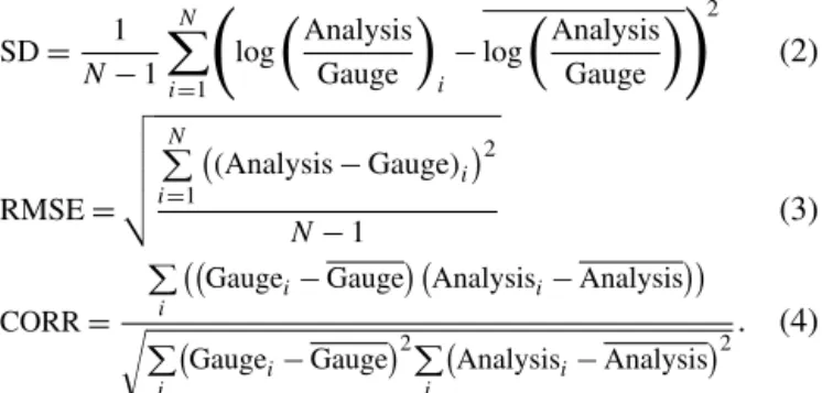
beam is 5 km wide at a distance of 250 km). The validation of the different analysis methods is based on the logarithmic standard deviation (SD; Eq. 2), root mean square deviation (RMSE; Eq. 3) and Pearson’s correlation coefficient (CORR; Eq. 4):
SD= 1 N−1
N
X
i=1
log Analysis Gauge i −log Analysis Gauge !2 (2) RMSE= v u u u t N P
i=1
(Analysis−Gauge)i
2
N−1 (3)
CORR=
P
i
Gaugei−Gauge
Analysisi−Analysis
r P
i
Gaugei−Gauge
2P
i
Analysisi−Analysis
2 . (4)
SD quantifies the amount of variation (i.e., spread) of a dataset. A low SD indicates that the data points tend to be close to the mean value of the dataset. Here, we use the log-arithm of the quotients, in order to get the datasets closer to be normally distributed. RMSE is a quadratic scoring rule which measures the average magnitude of the error. Since the errors are squared before they are averaged, RMSE gives a relatively high weight to large errors. CORR gives a mea-sure of the linear relationship (both strength and direction) between two quantities.
4 Results
Verification results using lightning data are presented in Sect. 4.1 and the impact from different integration time in-tervals in Sect. 4.2.
4.1 FMI-LAPS LDA results
The verification for the entire summer of 2015, i.e., using verification dataset (a) including days with no thunderstorms, assures that introducing lightning data has no significant im-pact on the overall performance of the system. The imim-pact of using the LDA method for estimating the precipitation accu-mulation is neutral for this long verification period (shown in Fig. 4, where the data are from dependent stations). The same result is seen in the scores of RMSE, SD and CORR values (not included here). Since the data have been much influenced by weather situations not related to lightning, the focus will be on the subsets, i.e., datasets (c) and (d), the 25-day periods of intense lightning 25-days of both 2015 and 2016, respectively.
The 25-day period with frequent thunderstorms dur-ing summer 2015, verification dataset (c), for which we used the average method to calculate the Rad_Lig pro-files, shows an inconsistent result using lightning data (see Table 1, left column). For the independent dataset, the Rad_LDA_Accum has a slightly improved result (lower RMSE value) when compared with Rad_Accum. On the other hand, Rad_LDA_RandB gets worse results, as can be seen from the RMSE and CORR. The dependent data show almost neutral impact (RMSE is slightly better for Rad_LDA_RandB) with the use of the LDA method and av-erage calculated Rad-Lig profiles.
Figure 5 shows the results using verification dataset (e), where different Rad-Lig profiles are compared (e.g., average, third quartile and variable quartile profiles) and validated against Rad_Accum. The precipitation accumulation esti-mates are improved at high accumulation values (> 5 mm) us-ing either third or variable quartile profiles. Simultaneously, they both add to the overestimate in low accumulation values (< 5 mm). The third quartile profiles give the largest overesti-mate over the whole accumulation scale. The variable quar-tile gives the overall best result, with improved estimates for high accumulation values and only slight overestimation at low values.
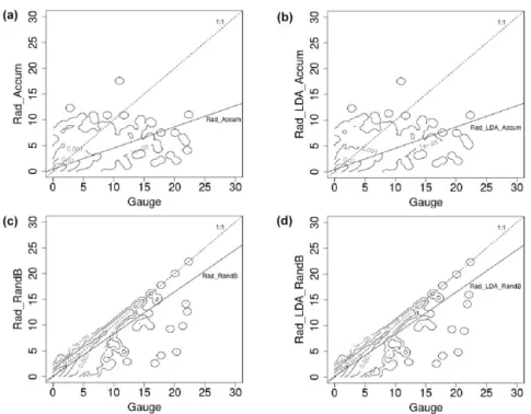
Figure 4.The FMI-LAPS precipitation accumulation (described in plots with density isolines of hourly accumulation values in millime-ters) calculated using four different methods. Fit in solid line (see regression equations), the perfect solution would align on the 1:1 dashed line:(a)Rad_Accum (y=0.410x+0.398),(b)Rad_LDA_Accum (y=0.413x+0.396),(c)Rad_RandB (y=0.817x+0.093) and (d)Rad_LDA_RandB (y=0.819x+0.091). Results are from the dependent gauge dataset during summer 2015, i.e., verification dataset (a).
Table 1.Precipitation accumulation results from summer of 2015 (i.e., dataset c, left column) and 2016 (i.e., dataset d, right column), for periods of the 25 intensive lightning days (e.g., > 100 CG strokes per day) during both years. Precipitation results are shown for radar (Rad_Accum) and radar merged with lightning data (Rad_LDA_Accum), together with and without gauge measurements included with the RandB method (Rad_RandB and Rad_LDA_RandB, respectively). In the lowest panels, only data from more than 100 or 150 km from the nearest radar are used. Verification is performed against both independent and dependent stations, i.e., those used or left out from the gauge analysis.
Summer 2015 (average scheme) Summer 2016 (variable quartile scheme)
Independent Rad_ Rad_LDA_ Rad_ Rad_LDA_ Independent Rad_ Rad_LDA_ Rad_ Rad_LDA_ Accum Accum RandB RandB Accum Accum RandB RandB
No. obs 3206 3332 256 256 No. obs 1320 1333 74 74
SD 0.27 0.27 0.11 0.11 SD 0.32 0.32 0.12 0.11
RMSE 1.66 1.64 0.58 0.70 RMSE 2.62 2.60 0.92 0.89
CORR 0.67 0.67 0.97 0.96 CORR 0.64 0.65 0.96 0.96
Dependent Dependent
No. obs 3566 3567 No. obs 1364 1376
SD 0.12 0.12 SD 0.14 0.13
RMSE 0.77 0.76 RMSE 1.27 1.19
CORR 0.93 0.93 CORR 0.93 0.94
> 100 km > 100 km
No. obs No. obs 656 656 694 698
SD SD 0.34 0.34 0.15 0.15
RMSE RMSE 2.44 2.39 1.03 1.01
CORR CORR 0.66 0.67 0.95 0.95
> 150 km > 150 km
No. obs No. obs 153 153 168 171
SD SD 0.39 0.39 0.20 0.20
RMSE RMSE 2.46 2.42 1.47 1.43
Figure 5. Verification of hourly accumulation values for Rad_Accum (black squares, with regression line equation y=
0.349x+0.638) and LDA_Accum (triangle, cross and circular markers), using three different methods to calculate the relationship profiles: average (blue triangles,y=0.360x+0.691), third quartile (red circles, y=0.417x+0.844) and the variable quartile (green crosses, y=0.365x+0.710) accumulation estimates. The corre-sponding regression lines (see equations) are represented with same color as the markers for each method. Data are for the 4-day period in summer 2014, i.e., verification dataset (e). The best-fit curve (i.e., the 1 : 1 fit) is shown as a black solid line.
and increased CORR values for Rad_LDA_Accum com-pared to Rad_Accum. Also, Rad_LDA_RandB gets smaller errors than Rad_RandB (see SD and RMSE in Table 1, most upper-right panel). For the dependent stations, all scores are improved using the LDA method, especially the RMSE (as seen in Table 1, right column, second panel). The verifi-cation of distance dependencies, i.e., for observations fur-ther away than 100 and 150 km from the nearest radar sta-tions, shows improved accumulation estimates when using the LDA method (see Table 1, right column, two last pan-els). The RMSE and CORR scores for Rad_LDA_Accum and Rad_LDA_RandB are better than Rad_Accum and Rad_RandB, respectively. Here, only dependent gauges are available for verification.
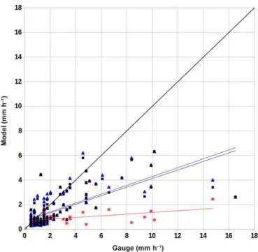
Comparing accumulation results from the 4-day period, i.e., verification dataset (e), for radar alone (Rad_Accum; black markers in Fig. 6) and lightning alone (LDA_Accum; red markers in Fig. 6), it is clear that the use of LDA_Accum is less accurate than Radar_Accum results. Figure 6 also shows that the Rad_LDA_Accum estimates (using the base-line method, with average Rad-Lig profiles) are amplified over the whole range of precipitation values, compared to
Figure 6. Verification of hourly accumulation values for LDA_Accum (red stars, with regression line equationy=0.068x+
0.685) and the merged Rad_LDA_Accum (blue triangles, y=
0.360x+0.691), compared to Rad_Accum (black boxes, y=
0.349x+0.638). The corresponding regression lines (see equations) are represented with same color as the markers for each method. Data are for the 4-day period in summer 2014, i.e., verification dataset (e). The black solid line is the best-fit line (1 : 1 fit).
Rad_Accum (Fig. 6; compare the blue with the black mark-ers). For the high accumulation values (> 5 mm h−1), this is a positive effect, while in the lower range (< 5 mm h−1) there is an overestimation of the results.
4.2 RandB method and impact from different integration periods
Figure 7.Impact of changing the integration time length, with verification for the independent gauges, using verification dataset (a) from sum-mer 2015. Accumulation plots with density isolines of hourly values in millimeters:(a)Rad_LDA_Accum (with regression line equationy=
0.594x−0.312),(b)Rad_LDA_RandB (y=0.891x−0.147),(c)Rad_LDA_RandB_6hr (y=0.732x−0.160),(d)Rad_LDA_RandB_12hr (y=0.725x−0.169),(e)Rad_LDA_RandB_24hr (y=0.715x−0.167) and(f)Rad_LDA_RandB_7d (y=0.692x−0.166). The fit is shown in solid lines (see regression equations); the perfect solution would align on the 1 : 1 dashed line.
Table 2.Impact of the integration time length on the RandB method for the dependent and independent stations datasets during summer 2015, i.e., dataset (a). The Rad_LDA_Accum (e.g., a method not using RandB) is included as a reference.
Dependent Rad_LDA_ Rad_LDA_ Rad_LDA_ Rad_LDA_ Rad_LDA_ Rad_LDA_ Accum RandB_1hr RandB_6hr RandB_12hr RandB_24hr RandB_7d
No. of observations 13 200 16 311 10 956 10 917 10 915 11 033
SD (log(R/G)) 0.25 0.13 0.13 0.13 0.14 0.14
RMSE 1.20 0.52 0.67 0.71 0.72 0.72
CORR 0.64 0.93 0.91 0.90 0.89 0.89
Independent
No. of observations 1177 1492 1028 1013 1005 1014
SD (log(R/G)) 0.25 0.15 0.22 0.22 0.22 0.22
RMSE 1.38 0.68 1.16 1.23 1.24 1.24
5 Discussions and conclusions
The aim of this article is to describe new methods on how to improve the hourly precipitation accumulation estimates, especially for heavy rainfall events (> 5 mm) and as much as possible for the low-valued ranges (< 5 mm).
The strength of the LDA method is that the radar and light-ning information can be merged and complement each other. This is especially important in areas of poor or even non-existent radar coverage, where the lightning information will improve the reflectivity field and thereby the hourly precipi-tation accumulation analysis. It is important to recall that, in the LAPS accumulation process, the reflectivity field is the first step, which is then corrected with gauges (e.g., if there is no reflectivity field, gauges will not be used and there will be no accumulation field). The results in this article are lim-ited to Finland but should this area be extended to include Scandinavia, the LDA method will become even more use-ful. There are also other LAPS users in other parts of the world, whom we want to encourage to continue this work.
The whole summer periods of 2015 and 2016 show neu-tral impact on the results using the LDA method; scores are not included here but Fig. 4 shows the graphs for tion dataset (a). It is important to make long-term verifica-tion in order to see that the system is robust and does not generate any bad data during any weather situation, i.e., per-form a sanity check of the system. However, in order to nar-row down our analysis to areas and times where lightning did occur (i.e., exclude stratiform precipitation), we focused our results on the subset of 25 lightning intensive days for both 2015 and 2016, datasets (c) and (d), respectively. The subset of 2015, using the average method, gave inconsistent results and no unambiguous conclusions could be drawn (Table 1, left column).
New methods to calculate the Rad-Lig profiles were tested and reveal that the variable quartile method improves the es-timates for the large accumulation (i.e., > 5 mm), though with some overestimation in low accumulation (Fig. 5). The third quartile approach has the highest impact on the whole accu-mulation field, which results in large overestimates for the low accumulation values (i.e., 0–5 mm). The average method smoothes out the small-scale variances, which are observed in heavy convection. Hence, the collected radar reflectivity profiles are less representative, and therefore the calculated Rad-Lig profiles will have values that are too low in these cases. As a result, the average method will have a low im-pact on the final precipitation accumulation estimates, com-pared to the use of the third quartile and variable quartile methods (Fig. 5). One should also mention that there is an overall uncertainty due to instrumental errors and the collo-cation between observations within the LDA method. This could potentially result in dislocation and bad quality of the received radar and lightning measurements, which would af-fect the calculated Rad-Lig profiles (for example, in the event of radar attenuation, where strong rainfall weakens some part
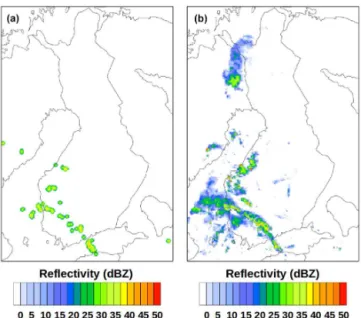
Figure 8. Reflectivity field simulated from lightning data alone (left) and, for verification, from radar data alone (right) 30 July 2014 at 16:00 UTC. The reflectivity color scale is shown below plots.
of the reflectivity field). Here, the collected radar profiles will have reflectivity values that are too low and give underesti-mated Rad-Lig profiles, especially when using the average method.
The newest results from 2016 and the 25-day subset show that there is a benefit to using the LDA (variable quartile) method. Mainly, all scores are becoming better and few are unchanged when lightning information is used to estimate the precipitation accumulation (see Table 1, right column). Veri-fying the dataset with distance to radar stations (i.e., gauges situated further away than 100 and 150 km) also shows the same results; the accumulation product is improved with the LDA method. The impact on scores is mainly in the second decimal, but they are consistent, and clearly show the ten-dency of improvement by using the LDA method with the variable quartile profiles. One reason we do not see a larger impact by the LDA method could be that the Finnish radar network does have a very high quality and system utilization rate and therefore is less impacted by the LDA method. In an upcoming version of FMI-LAPS, the verification will be focusing on including areas with poor (or non-existent) radar coverage where gauges are available.
and this could have an effect on the methodology used here. In future developments, after collecting longer time series to quantify the nature of uncertainty of lightning-based precip-itation estimates, we intend to improve the analysis in this direction.
In the present analysis area, we mainly anticipate the use-fulness of lightning data as a backup plan of rare but signifi-cant cases. Due to the rare nature of such events, it is not pos-sible to collect a statistically representative dataset in a few years; even though attenuation of radar signals or completely missing data are observed several times a summer, it is not so often that such events happen just over a rain gauge station. However, our overall analysis shows that when we include the lightning data every day at every point, they make, on average, a small improvement, and they are there as a safety network waiting for the cases where radars fail.
For the near-real-time accumulation product, data used from the recent hour of analysis time do give the best pre-cipitation accumulation result (Table 2 and Fig. 7). We see correlation peaking at the 1 h integration period and decreas-ing already for the 6 h period. Therefore, accorddecreas-ing to the results in this study, the use of long time integration periods for the RandB method (until 7 days in this case) does not im-prove the hourly precipitation accumulation analysis. Berndt et al. (2014) compared data resolutions from 10 min to 6 h and reported a large improvement in the correlation (from 10 min to 1 h, the correlation increased 0.37 to 0.57). From 1 to 6 h, the corresponding increase was 0.57 to 0.62, respec-tively. In Norway, Abdella and Alfredsen (2010) have shown that the use of average monthly adjustment factors leads to less than optimal results. One could speculate that there is an intermediate choice of temporal resolution that would im-prove the results in this article. For example, there could be better results using periods of 2 to 5 h. This has not been investigated in this article but will be considered in future studies.
6 Data availability
LAPS source code, including the LDA method, is available from NOAA (2017). The materials and data used in this
ar-References
Aaltonen, J., Hohti, H., Jylhä, K., Karvonen, T., Kilpeläinen, T., Koistinen, J., Kotro, J., Kuitunen, T., Ollila, M., Parvio, A., Pulkkinen, S., Silander, J., Tiihonen, T., Tuomenvirta, H., and Vajda, A.: Strong precipitation and urban floods (Rankkasateet ja taajamatulvat RATU), Finnish Environment Institute (Suomen ympäristókeskus), Helsinki, Finland, 80 pp., 2008.
Abdella, Y. and Alfredsen, K.: Long-term evaluation of gauge-adjusted precipitation estimates from a radar in Norway, Hydrol. Res., 41, 171–192, 2010.
Albers, S. C., McGinley, J. A., Birkenheuer, D. L., and Smart, J. R.: The local analysis and prediction system (LAPS): Analyses of clouds, precipitation, and temperature, Weather Forecast., 11, 273–287, 1996.
Battan, L. J.: Radar Observation of the Atmosphere, University of Chicago Press, Chicago, USA, 1973.
Berndt, C., Rabiei, E., and Haberlandt, U.: Geostatistical merging of rain gauge and radar data for high temporal resolutions and vari-ous station density scenarios, J. Hydrology, 508, 88–101, 2014. Cummins, K. L., Murphy, M. J., Bardo, E. A., Hiscox, W. L., Pyle,
R. B., and Pifer, A. E.: A combined TOA/MDF technology up-grade of the U.S. National Lightning Detection Network, J. Geo-phys. Res., 103, 9035–9044, doi:10.1029/98JD00153, 1998. Einfalt, T., Jessen, M., and Mehlig, B.: Comparison of radar and
raingauge measurements during heavy rainfall, Water Sci. Tech-nol., 51, 195–201, 2005.
Germann, U.: Radome attenuation – a serious limiting factor for quantitative radar measurements?, Meteorol. Z., 8, 85–90, 1999. Gires, A., Tchiguirinskaia, I., Schertzer, D., Schellart, A., Berne, A., and Lovejoy, S.: Influence of small scale rainfall variability on standard comparison tools between radar and rain gauge data, At-mos. Res., 138, 125–138, doi:10.1016/j.atmosres.2013.11.008, 2014.
Goudenhoofdt, E. and Delobbe, L.: Evaluation of radar-gauge merging methods for quantitative precipitation estimates, Hy-drol. Earth Syst. Sci., 13, 195–203, doi:10.5194/hess-13-195-2009, 2009.
Gregow, E., Saltikoff, E., Albers, S., and Hohti, H.: Precipitation ac-cumulation analysis – assimilation of radar-gauge measurements and validation of different methods, Hydrol. Earth Syst. Sci., 17, 4109–4120, doi:10.5194/hess-17-4109-2013, 2013.
Jaffrain, J. and Berne, A.: Influence of the subgrid variability of the raindrop size distribution on radar rainfall estimators, J. Appl. Meteorol. Clim., 51, 780–785, doi:10.1175/JAMC-D-11-0185.1, 2012.
Jewell, S. A. and Gaussiat, N.: An assessment of kriging-based rain-gauge-radar merging techniques, Q. J. Roy. Meteor. Soc., 141, 2300–2313, doi:10.1002/qj.2522, 2015.
Koistinen, J. and Michelson, D. B.: BALTEX weather radar-based precipitation products and their accuracies, Boreal Environ. Res., 7, 253–263, 2002.
Koskinen, J. T., Poutiainen, J., Schultz, D. M., Joffre, S., Koisti-nen, J., Saltikoff, E., Gregow, E., TurtiaiKoisti-nen, H., Dabberdt, W. F., Damski, J., Eresmaa, N., Göke, S., Hyvärinen, O., Järvi, L., Karppinen, A., Kotro, J., Kuitunen, T., Kukkonen, J., Kulmala, M., Moisseev, D., Nurmi, P., Pohjola, H., Pylkkö, P., Vesala, T., and Viisanen, Y.: The Helsinki Testbed: A mesoscale measure-ment, research, and service platform, B. Am. Meteorol. Soc., 92, 325–342, doi:10.1175/2010BAMS2878.1, 2011.
Mäkelä, A., Tuomi, T. J., and Haapalainen, J.: A decade of high-latitude lightning location: Effects of the evolving lo-cation network in Finland, J. Geophys. Res., 115, D21124, doi:10.1029/2009JD012183, 2010.
Mäkelä, A., Rossi, P., and Schultz, D. M.: The daily cloud-to-ground lightning flash density in the contiguous United States and Finland, Mon. Weather Rev., 139, 1323–1337, doi:10.1175/2010MWR3517.1, 2011.
Mäkelä, A., Mäkelä, J., Haapalainen, J., and Porjo, N.: The veri-fication of lightning location accuracy in Finland deduced from lightning strikes to trees, Atmos. Res., 172, 1–7, 2016.
Marshall, J. S. and Palmer, W. M.: The Distribution of raindrops with size, J. Meteorol., 5, 165–166, 1948.
Morales, C. A. and Anagnostou, E. N.: Extending the capabilities of high-frequency rainfall estimation from geostationary-based satellite infrared via a network of long-range lightning observa-tions, J. Hydrometeorol., 4, 141–159, 2003.
NOAA: Latest release of LAPS software, available at: http://laps. noaa.gov/cgi/LAPS_SOFTWARE.cgi, last access: 11 January 2017.
Papadopoulos, A., Chronis, T. G., and Anagnostou, E. N.: Improv-ing convective precipitation forecastImprov-ing through assimilation of regional lightning measurements in a mesoscale model, Mon. Weather Rev., 133, 1961–1977, 2005.
Pessi, A.: Characteristics of Lightning and Radar Reflectivity in Continental and Oceanic Thunderstorms, 93th Annual American Meteorological Society Meeting, Austin, Texas, USA, 6–10 Jan-uary 2013, availabe at: https://ams.confex.com/ams/93Annual/ webprogram/Paper215562.html (last access: 9 January 2017), 2013.
Pessi, A. and Albers, S.: A Lightning Data Assimilation Method for the Local Analysis and Prediction System (LAPS): Impact on Modeling Extreme Events, 94th Annual American Meteo-rological Society Meeting, Atlanta, Georgia, USA, 1–6 Febru-ary, 2014, available at: https://ams.confex.com/ams/94Annual/ webprogram/Paper238715.html (last access: 9 January 2017), 2014.
Pessi, A. and Businger, S.: The Impact of Lightning Data Assimila-tion on a Winter Storm SimulaAssimila-tion over the North Pacific Ocean, Mon. Weather Rev., 137, 3177–3195, 2009.
Said, R. K., Inan, U. S., and Cummins, K. L.: Long-range lightning geolocation using a VLF radio atmospheric waveform bank, J. Geophys. Res., 115, D23108, doi:10.1029/2010JD013863, 2010. Saltikoff, E., Huuskonen, A., Hohti, H., Koistinen, J., and Järvi-nen, H.: Quality assurance in the FMI Doppler Weather radar network, Boreal Environ. Res., 15, 579–594, 2010.
Schiemann, R., Erdin, R., Willi, M., Frei, C., Berenguer, M., and Sempere-Torres, D.: Geostatistical radar-raingauge combi-nation with nonparametric correlograms: methodological consid-erations and application in Switzerland, Hydrol. Earth Syst. Sci., 15, 1515–1536, doi:10.5194/hess-15-1515-2011, 2011. Sideris, I. V., Gabella, M., Erdin, R., and Germann, U.: Real-time
radar-raingauge merging using spatiotemporal co-kriging with external drift in the alpine terrain of Switzerland, Q. J. Roy. Me-teor. Soc., 140, 1097–1111, 2014.
Tuomi, T. J. and Mäkelä, A.: Lightning observations in Finland, Reports, Finnish Meteorological Institute, Helsinki, Finland, 2007:5, 49 pp, 2007.
Tuomi, T. J. and Mäkelä, A.: Thunderstorm climate of Finland 1998–2007, Geophysica, 44, 29–42, 2008.
Uijlenhoet, R.: Raindrop size distributions and radar reflectivity– rain rate relationships for radar hydrology, Hydrol. Earth Syst. Sci., 5, 615–628, doi:10.5194/hess-5-615-2001, 2001.
Wang, L.-P., Ochoa-Rodríguez, S., Onof, C., and Willems, P.: Singularity-sensitive gauge-based radar rainfall adjustment methods for urban hydrological applications, Hydrol. Earth Syst. Sci., 19, 4001–4021, doi:10.5194/hess-19-4001-2015, 2015. Wilson, J. W. and Brandes, E. A.: Radar Measurement of Rainfall –