Correcting the radar rainfall forcing of a hydrological model with data assimilation: application to flood forecasting in the Lez Catchment in Southern France

(1)

HESSD

9, 3527–3579, 2012

Data assimilation for the correction of

radar rainfall

E. Harader et al.

Title Page

Abstract Introduction

Conclusions References

Tables Figures

◭ ◮

Back Close

Full Screen / Esc

Printer-friendly Version Interactive Discussion

Discussion

P

a

per

|

Dis

cussion

P

a

per

|

Discussion

P

a

per

|

Discussio

n

P

a

per

|

Hydrol. Earth Syst. Sci. Discuss., 9, 3527–3579, 2012 www.hydrol-earth-syst-sci-discuss.net/9/3527/2012/ doi:10.5194/hessd-9-3527-2012

Hydrology and Earth System Sciences Discussions

This discussion paper is/has been under review for the journal Hydrology and Earth System Sciences (HESS). Please refer to the corresponding final paper in HESS if available.

Correcting the radar rainfall forcing of a

hydrological model with data

assimilation: application to flood

forecasting in the Lez Catchment in

Southern France

E. Harader1,2, V. Borrell Estupina2, S. Ricci1, M. Coustau2, O. Thual1,3, A. Piacentini1, and C. Bouvier2

1

URA CERFACS-CNRS, URA1875, Toulouse, France 2

HSM, UMR5569 CNRS IRD UM1 UM2, Montpellier, France 3

INPT, CNRS, IMFT, Toulouse, France

Received: 21 February 2012 – Accepted: 5 March 2012 – Published: 15 March 2012 Correspondence to: E. Harader (harader@cerfacs.fr)

(2)

HESSD

9, 3527–3579, 2012

radar rainfall

E. Harader et al.

Title Page

Tables Figures

◭ ◮

Back Close

Full Screen / Esc

Discussion

P

a

per

|

Dis

cussion

P

a

per

|

Discussion

P

a

per

|

Discussio

n

P

a

per

|

Abstract

The present study explores the application of a data assimilation (DA) procedure to correct the radar rainfall inputs of an event-based, distributed, parsimonious hydrologi-cal model. A simplified Kalman filter algorithm was built on top of a rainfall-runoffmodel in order to assimilate discharge observations at the catchment outlet. The study site

5

is the 114 km2 Lez Catchment near Montpellier, France. This catchment is subject to heavy orographic rainfall and characterized by a karstic geology, leading to flash flooding events. The hydrological model uses a derived version of the SCS method, combined with a Lag and Route transfer function. Because it depends on geographical features and cloud structures, the radar rainfall input to the model is particularily

uncer-10

tain and results in significant errors in the simulated discharges. The DA analysis was applied to estimate a constant correction to each event hyetogram. The analysis was carried out for 19 events, in two different modes: re-analysis and pseudo-forecast. In both cases, it was shown that the reduction of the uncertainty in the rainfall data leads to a reduction of the error in the simulated discharge. The resulting correction of the

15

radar rainfall data was then compared to the mean field bias (MFB), a corrective coef-ficient determined using ground rainfall measurements, which are more accurate than radar but have a decreased spatial resolution. It was shown that the radar rainfall cor-rected using DA leads to improved discharge simulations and Nash criteria compared to the MFB correction.

20

1 Introduction

For flash flood prediction, hydrologists may use tools as rudimentary as rainfall-discharge curves or as refined as complex physical and distributed hydrological models, all with the goal of converting atmospheric and soil conditions into discharge volumes, flood peak amplitudes and arrival times. All of these tools are subject to uncertainties related

25

(3)

HESSD

9, 3527–3579, 2012

radar rainfall

E. Harader et al.

Title Page

Tables Figures

◭ ◮

Back Close

Full Screen / Esc

Discussion

P

a

per

|

Dis

cussion

P

a

per

|

Discussion

P

a

per

|

Discussio

n

P

a

per

|

quantities and their spatial distribution throughout the catchment, as runoffgeneration depends upon rainfall location. Errors in rainfall estimates have a significant impact on prevision and event reconstruction quality. In studies of flash flood modelling for Roma-nian catchments between 36 and 167 km2, Zoccatelli et al. (2010) demonstrated that neglecting rainfall spatial variability resulted in a deterioration of the simulation

qual-5

ity. Roux et al. (2011) showed that the MARINE model (Estupina-Borrell, 2004) was dependent upon the distribution of rainfall data in order to correctly represent the soil saturation dynamics of the 545 km2Gardon d’Anduze Catchment in Southern France. Finally, in a study of the 2002 flash flood in the Gard Department of Southern France, Anquetin et al. (2010) demonstrated that the spatial resolution provided by radar

rain-10

fall was necessary for the correct representation of flood dynamics in catchments with areas from 2.5 to 99 km2.

The sensitivity of models to rainfall distribution highlights the importance of using a rainfall product with a fine spatial and temporal resolution, such as radar rainfall. However, depending on the characteristics of the model and the storm event, finely

re-15

solved radar rainfall may have a variable effect on hydrological behavior and can result in either improvement or degradation of the simulation quality (Tetzlaffand Uhlenbrook, 2005; Anquetin et al., 2010). As demonstrated by Tetzlaffand Uhlenbrook (2005), radar rainfall often degrades simulation efficiency, except in the case of highly variable con-vective events, due to decreased data quality with radar. Using a physically-based,

20

distributed model, Anquetin et al. (2010) showed that simulation error increases with the ratio of the rainfall length scale to the catchment scale, arguing for the necessity of radar rainfall. However, properly calibrated lumped models can outperform distributed models when radar rainfall is relatively uniform over the basin (Smith et al., 2004).

The use of radar data is often limited by increased uncertainties compared to ground

25

(4)

HESSD

9, 3527–3579, 2012

radar rainfall

E. Harader et al.

Title Page

Tables Figures

◭ ◮

Back Close

Full Screen / Esc

Discussion

P

a

per

|

Dis

cussion

P

a

per

|

Discussion

P

a

per

|

Discussio

n

P

a

per

|

mountainous regions based on distance considerations, as done so for the HYDRAM rainfall product used in this study, leads to a lower quality rainfall product compared to using a composite (highest quality scan at any given point) method (Cheze and Hel-loco, 1999). Additionally, in the Lez Catchment, radar data quality varies by season and is diminished in winter months due to bright band e_ffects related to predominantly

strat-5

iform rainfall (Coustau et al., 2011; Emmanuel et al., 2012; Tabary, 2007). Techniques for removing bright band effects are foreseen in the next generation M ´et ´eo-France rain-fall product (PANTHERE), which will help to improve winter rainrain-fall.

A possible post-treatment correction to radar rainfall is the removal of the mean field bias (MFB) (Wilson and Brandes, 1979), a correction which uses gauge data to

elim-10

inate errors due to instrumentation and a non-linear vertical profile reflectivity (VPR). Adjustment of radar rainfall using gauge data has been shown to lead to improved pre-diction accuracy (Vieux and Bedient, 2004; Cole and Moore, 2008). Building on this approach, Kahl and Nachtnebel (2008) implemented a technique which corrects radar rainfall using a correction plane in which the coefficients are determined by minimizing

15

an objective function.

Identifying a correction to the rainfall data input to hydrological models can also be formulated as an inverse problem (Tarantola, 2005; McLaughlin and Townley, 1996) conveniently solved in the framework of data assimilation. Data assimilation is a math-ematical technique inherited from estimation theory, initially developped for

meteoro-20

logical applications, that combines measurements with model simulations in order to improve the numerical prediction of a system. Data assimilation leads to an optimal es-timation of the set of parameters, initial or boundary conditions which allow the model to accurately represent the system.

Data assimilation for the improvement of hydrological event reconstruction or

fore-25

(5)

HESSD

9, 3527–3579, 2012

radar rainfall

E. Harader et al.

Title Page

Tables Figures

◭ ◮

Back Close

Full Screen / Esc

Discussion

P

a

per

|

Dis

cussion

P

a

per

|

Discussion

P

a

per

|

Discussio

n

P

a

per

|

Meier et al., 2011). Chumchean et al. (2006) applied a Kalman filter technique (Bouttier and Courtier, 1999) to the calculation of the mean field bias with the use of an autore-gressive (AR) function to model the time evolution of the MFB; this technique resulted in a reduction in the error associated with the MFB when given sufficient rain gauge data.

5

Previous studies have adopted a variety of approaches to implementing the Kalman Filter algorithm. A common factor of these non-variational data assimilation applica-tions is that errors in the model states or parameters are assumed to follow Bayesian statistics and their probability density functions are determined recursively. The Kalman Filter explicitly propagates these errors in time, assuming a linear dynamic model. The

10

Extended Kalman Filter (EKF) re-estimates the Jacobian of the dynamic model at each new time step in order to address possible non-linearities in the evolution of the errors (Goegebeur and Pauwels, 2007). In systems where the error covariances are either di_fficult to define or the computational cost to propagate them is too great, the En-semble Kalman Filter (EnKF) estimates the error covariance at each timestep using

15

the ensemble members (Weerts and El Serafy, 2006; Pauwels and De Lannoy, 2009). The use of ensemble methods, however, comes at the cost of greatly increasing the number of model runs. The simplified version of the version of the Kalman Filter used in this study is applied over a single time window covering either the entire flood event or the start of the flood event and with a scalar control vector containing a corrective

coef-20

ficient to the input rainfall. The background error variance is predefined using the MFB and does not evolve in time, thus avoiding the need for an EKF or ensemble approach. These simplifications are adapted to the correction of time-invariant parameters which should not evolve over the course of the rainfall event.

In this paper, discharge observations are assimilated with a simplified Kalman Filter

25

(6)

HESSD

9, 3527–3579, 2012

radar rainfall

E. Harader et al.

Title Page

Tables Figures

◭ ◮

Back Close

Full Screen / Esc

Discussion

P

a

per

|

Dis

cussion

P

a

per

|

Discussion

P

a

per

|

Discussio

n

P

a

per

|

correction is assumed to remain constant. The state variables, outputs, inputs or pa-rameters to be corrected are gathered into a control vector, which in this case contains only the constant rainfall corrective coefficient. The observation operator mapping the control vector onto the observation space is represented by the integration of the hy-drological model. The KF algorithm relies on the hypothesis that the relation between

5

the rainfall corrective parameter and the discharge at the catchment outlet is fairly lin-ear. In our study, an outer loop procedure was applied to account for some of the non-linearities in this relation. The analysis was carried out for 19 heavy rainfall events occuring within the Lez catchment in Southern France between 1997 and 2008. The events were of variable intensity and had measured peak flows between approximately

10

10–400 m3s−1 at the watershed outlet. It was shown that the reduction of the uncer-tainty in the rainfall data leads to a reduction of the error in the simulated discharge and that the radar rainfall corrected using DA leads to improved discharge simulations and Nash criteria, over the MFB correction.

The paper is outlined as follows: Sect. 2 explores pertinent hydrological features of

15

the Lez Catchment and the structure of the hydrological model. The DA procedure is presented in Sect. 3. The results of the study and the impacts of data assimilation upon the efficiency of the hydrological model are described in Sect. 5. Finally, a summary of the key results obtained and suggestions for future research directions are presented in Sect. 6.

20

2 Study site and hydrological model description

2.1 The Lez Catchment

The Lez Catchment in Southern France (Fig. 1) is a medium sized karstic basin located 15 km north of the town of Montpellier. The catchment is 114 km2 at Lavalette, where discharge measurements are taken. This portion of the Lez river is fed by several

25

(7)

HESSD

9, 3527–3579, 2012

radar rainfall

E. Harader et al.

Title Page

Tables Figures

◭ ◮

Back Close

Full Screen / Esc

Discussion

P

a

per

|

Dis

cussion

P

a

per

|

Discussion

P

a

per

|

Discussio

n

P

a

per

|

downstream of Lavalette, such as the Mosson, the Lironde and the Verdanson were not taken into account in this study. If the Mosson tributary is included, the catchment drains a total of 560 km2. This larger catchment includes the town of Montpellier which extends from the gauging station at Lavalette in the North to the Mauguio rain gauge in the South.

5

The Lez River flows for a total of 26 km before emptying into the Mediterranean Sea. The riparian area of the Lez Hydrosystem has been extensively developed downstream of the town of Castelnau-le-Lez and continuing into the estuary, Etangs-Palavasiens. The undeveloped stretch of the Lez river extends for 10–15 km from the source to Castelnau-le-Lez and has an average slope of 3 ‰, compared to less than 1 ‰ in

10

developed areas.

The landscape of the Lez Catchment at Lavalette is defined by plains and hilly gar-rigue with limestone outcrops and very little urbanisation. The plains are composed of 200 to 800 m thick Valanginian marls1, covered by soil usually less than 1 m thick. Land use ranges between agricultural (vineyards) and forest in the plains, along with

15

undeveloped garrigue; the limestone outcrops have very little soil cover and thin vege-tation.

2.1.1 The Karst system

The source of the Lez is a seasonal spring which serves as the main outlet of a 380 km2 limestone and dolomite karstic aquifer (shown by the dotted line in Fig. 1) (Avias, 1992).

20

When the spring pool reaches a level of₊65 m, it overflows into the Lez River. Sev-eral smaller seasonal springs drain the same system; these are discussed in greater detail in Fleury et al. (2009). The Lez Spring is actively pumped to provide water to the city of Montpellier. During the summer, part of the pumped flow is returned to the Lez River in order to maintain a minimum discharge of 160 l s−1. The aquifer is

25

1

(8)

HESSD

9, 3527–3579, 2012

radar rainfall

E. Harader et al.

Title Page

Tables Figures

◭ ◮

Back Close

Full Screen / Esc

Discussion

P

a

per

|

Dis

cussion

P

a

per

|

Discussion

P

a

per

|

Discussio

n

P

a

per

|

recharged during winter and fall by infiltration through the limestone outcrops as well as river losses (swallow holes).The recharge cycle appears to be sustainable, with no permanent impact to groundwater resources (Fleury et al., 2009).

Karstic systems are defined by the presence of conduits and fractures in the underly-ing limestone bedrock, resultunderly-ing in complex transport networks and variable response

5

times following rainfall events. The main surface processes considered to play a role in runoffgeneration in the watershed are soil depth and the slope of the hillside. The subsurface processes that contribute to runo_ffare poorly understood: they may reduce flood intensity by storing water in the epikarst and through deep inflitration (D ¨orfliger et al., 2008) or they may intensify the flood severity through the contribution of

ground-10

water to peak flow (Kong A Siou et al., 2011). The advanced study and modelling of the Lez karstic system is currently the subject of numerous research projects.

2.1.2 Climate and rainfall data

The climate of the region is generally dry, with mean annual evapotranspiration (1322 mm at Mauguio for the period 1996 to 2005 – Fig. 1) greater than mean annual rainfall

15

(909 mm at Prades for the period 1992 to 2008)2. Most of the yearly rainfall is re-ceived in fall and winter in the form of heavy climatic and orographic precipitations. Extreme rainfall events, particularly in fall and late summer periods, are favored in this region due to humidity generated by the warm Mediterranean Sea and a closed cy-clone which helps to transport warm, moist air masses to the coast (Nuissier et al.,

20

2008). In September of 2002, rainfall totaled as much as 600–700 mm in certain re-gions and resulted in destructive floods causing 24 deaths and 1.2 billion euros in economic damages (Boudevillain et al., 2011). The combination of intense autumnal rainfall and small karstic watersheds leads to dangerous flash flood conditions in the Mediterranean costal region.

25

2

(9)

HESSD

9, 3527–3579, 2012

radar rainfall

E. Harader et al.

Title Page

Tables Figures

◭ ◮

Back Close

Full Screen / Esc

Discussion

P

a

per

|

Dis

cussion

P

a

per

|

Discussion

P

a

per

|

Discussio

n

P

a

per

|

Rainfall in the Lez Catchment is measured by either an S-band radar located in Nˆımes at a distance of approximately 65 km from the basin or by a network of 4 rain-fall gauges (Prades, Montpellier-ENSAM, Maugio, Saint Martin de Londres – Fig. 1a). Radar data were treated using the HYDRAM algorithm developed by M ´et ´eo-France for the correction of ground clutters, the vertical profile of reflectivity, and conversion of

5

reflectivity to rainfall using the Marshall-Palmer relationship,

Z₌200R1.6, (1)

whereZ is the reflectivity in mm6m−3, R is the radar rainfall intensity in mm h−1 and 200 and 1.6 are empirical constants derived by the drop size distribution. For the HYDRAM treatment, the sameZ-R relationship is used for stratiform and convective

10

rainfall (Tabary, 2007). The Nˆımes radar produces scans at three different elevations at 5 min intervals: 2.5◦ (0–22 km), 1.3◦(22–80 km) and 0.6◦(distances beyond 80 km). These three different scans are used to produce a composite radar image which de-scribes rainfall for areas at different distances to the radar. The lowest unobstructed scan is selected for a given distance range. For the Lez Catchment, the 1.3◦scan was

15

used (Bouilloud et al., 2010) to produce cumulative rainfall depths at a spatial reso-lution of 1 km2 and a time step of 5 min. A network of 20 rain gauges within a 50 km range of the catchment provided cumulative rainfall data for adjustments using the MFB (Fig. 1b), a measure of the ratio of radar to rain gauge rainfall during a specified time period (here the length of the flood event):

20

MFB=

1

n P

iGi

1

n P

iRi

, (2)

whereG_i is the rain gauge measurement at location,i in mm,R_i is the radar measure-ment at the same location in mm andn is the number of rain gauges selected. The value of the radar measurement at the gauge location was selected to be the average of the central pixel and its 8 nearest neighbors. The ratio of rain gauge to radar

mea-25

(10)

HESSD

9, 3527–3579, 2012

radar rainfall

E. Harader et al.

Title Page

Tables Figures

◭ ◮

Back Close

Full Screen / Esc

Discussion

P

a

per

|

Dis

cussion

P

a

per

|

Discussion

P

a

per

|

Discussio

n

P

a

per

|

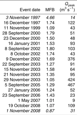
2.1.3 Rainfall events

Table 1 displays the 19 rainfall events measured by HYDRAM-treated radar for the Lez Catchment along with their associated MFB values and peak discharges. In general, events lasted several days and cumulative rainfall was sampled at a time step of 1 h. The episode MFBs were between 0.87 and 1.80, indicating that radar was never more

5

than 45 % away from the “true” rainfall value (assuming absolute confidence in ground measurements) with the exception of November 1997. The very high MFB for this event indicates that either the rain gauges, the radar or both were not functioning properly. With the exception of November 2008, all events have MFB values greater than 1, with an average of 1.39. As mentioned in Sect. 2.1.2, these values are a feature of the

10

distance between the Nˆımes radar and the watershed.

Rainfall events were separated into two classes based on their peak discharges: regular events which have a peak discharge greater than 40 m3s−1 and very small events which have a peak discharge less than or equal to 40 m3s−1. This classification is used to determine the range of discharges that will be assimilated as discussed in

15

Sect. 5.1.

2.2 The Hydrological model

The hydrological model is event-based, parsimonious and distributed. It operates on independant grid cells, using a SCS-derived runoffproduction function and a Lag and Route transfer function. Discharges are calculated using an hourly timestep in order to

20

(11)

HESSD

9, 3527–3579, 2012

radar rainfall

E. Harader et al.

Title Page

Tables Figures

◭ ◮

Back Close

Full Screen / Esc

Discussion

P

a

per

|

Dis

cussion

P

a

per

|

Discussion

P

a

per

|

Discussio

n

P

a

per

|

2.2.1 The runoffproduction function

The runoff production function is the link between the precipitation falling over the catchment and the discharge emitted to surface waters. Not all rain becomes dis-charge and processes such as infiltration, evapotranspiration, percolation and intercep-tion determine the eventual fate of incident rainfall. The ATHYS software, developed

5

by HydroSciences Montpellier (www.athys-soft.org), permits the use of several runoff

production functions, including Green & Ampt, TopModel, Girard, modified SCS and Smith & Parlange. From these options, a derived version of the SCS equations was selected for this study. The SCS model was originally created by engineers at the US Soil Conservation Service for use with small agricultural watersheds (less than 8 km2).

10

Numerous papers have been published demonstrating the utility of this model for pre-dicting runoffvolume (Abon et al., 2011; Sahu et al., 2007; Mishra and Singh, 2004). For predicting the instaneous runoffrate during an event, a derived version of the SCS equation is necessary. The derivation of the SCS function is shown below. The first use of these equations was performed by Gaume et al. (2004). The initial form of the

15

SCS equation is as follows,

V(t)= [Pb(t)−Ia]

2

P_b(t)−I_a₊SA, (3)

whereV is the cumulative runoffvolume generated by the watershed at timet in m3, I_ais the initial abstraction in mm,P_bis the cumulative rainfall depth at timetin mm, S is the potential storage depth of the watershed at the start of the event (potential

maxi-20

mum retention) in mm andAis the catchment area. For this study,P_bis considered as the level in a cumulative rainfall reservoir. Assuming an initial abstraction equal to 0.2S derived from studies of small rural watersheds (USDA Natural Resources Conserva-tion Service, 1986) and dividing by the area of the catchment, Eq. (3) reads,

P_e(t)₌ [Pb(t)−0.2S]

2

P_b(t)+0.8S , (4)

(12)

HESSD

9, 3527–3579, 2012

radar rainfall

E. Harader et al.

Title Page

Tables Figures

◭ ◮

Back Close

Full Screen / Esc

Discussion

P

a

per

|

Dis

cussion

P

a

per

|

Discussion

P

a

per

|

Discussio

n

P

a

per

|

whereP_e(t) is the cumulative runoffdepth generated by the watershed at timetin mm. Taking the time derivative of Eq. (4) leads to the instantaneous runo_ff rate (or runo_ff intensity) with units of mm s−1, denotedi_e(t). The time derivative ofP_b(t) is the rainfall rate (or rainfall intensity) in mm s−1, denoted i_b(t). The runoff intensity can now be described as a fraction of the rainfall intensity:

5

i_e(t)=i_b(t)Pb(t)−0.2S P_b(t)+0.8S

2−Pb(t)−0.2S

P_b(t)+0.8S

. (5)

Equation (5) has a form reminiscent of that described in the rational method (Doodge, 1957), which expresses the rate of runoff leaving the watershed outlet as a function of the percentage of area contributing to runoff, C(t), the rainfall rate and the area of the watershed. This method promotes the idea ofsaturation excess _{(Braud et al.,}

10

2010), where the contributing area is the soils which have been saturated and can no longer store water (Dunnian runoffgeneration). This is in contrast toinfiltration excess in which the soil’s capacity to allow incoming water to infiltrate is overcome and runoff

is generated while underlying soils remain unsaturated (Hortonian runoffgeneration). The equation of the rational method is shown below:

15

Q(t)=C(t)ib(t)A, (6)

whereQ(t) represents the runoffrate in m3s−1,C(t) is the proportion of the watershed contributing to runoff production, i_b(t) is the rainfall intensity in mm s−1 and A is the area in m2. Although the SCS method does not distinguish between Hortonian and Dunnian processes, thus making the physical meaning of its runoffproduction different

20

from that of the Rational Method, we can define the proportion of rainfall contributing to runoff,C(t), as follows,

C(t)= (_P

b(t)−0.2S P_b(t)+0.8S

2−Pb(t)−0.2S P_b(t)+0.8S

ifP_b(t)>0.2S

(13)

HESSD

9, 3527–3579, 2012

radar rainfall

E. Harader et al.

Title Page

Tables Figures

◭ ◮

Back Close

Full Screen / Esc

Discussion

P

a

per

|

Dis

cussion

P

a

per

|

Discussion

P

a

per

|

Discussio

n

P

a

per

|

The derived SCS method is thus convenient as it allows for the representation of runoff generation as a function of rainfall intensity throughout the event with param-eters that can be calibrated using physical measurements. This equation is valid for cumulative rainfalls greater than the initial abstraction. It should also be noted that the runoffcoefficient can never be greater than 1, meaning that runoffgeneration will never

5

exceed rainfall intensity:

lim

P_b(t)→∞C(t)=1. (8)

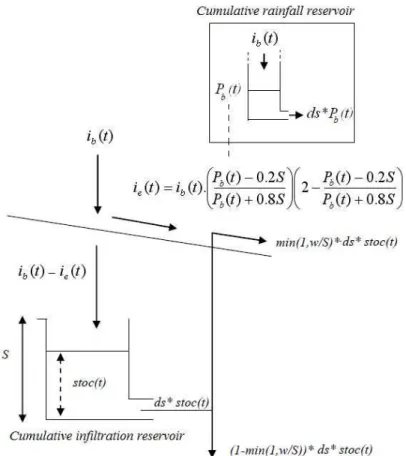
To represent the ability of the soil to regain part of its absorption potential during pauses in the rainfall, this version of the SCS method allows the soil to drain. The vol-ume of water lost to drainage is a function of two conceptual reservoirs: the cumulative

10

rainfall reservoir, levelP_b(t) and the soil reservoir, level stoc(t), shown in Fig. 3. The rate of drainage of the cumulative rainfall reservoir and the soil reservoir is described by:

dP_b(t)

dt =ib(t)−d s.Pb(t), (9)

15

dstoc(t)

dt =ib(t)−ie(t)−d s.stoc(t), (10)

whered s is the drainage coefficient. The coefficient represents the removal of water through deep infiltration and evapotranspiration during the event and is calculated from the slope of the descending limb of the hydrograph.

The drainage coefficients of the cumulative rainfall reservoir and the soil reservoir

20

were selected to be the same. The water lost to the system by the drainage coefficient is considered to be either lost to deep infiltration or to reemerge as delayed surface runoff,i_d(t), calculated by

i_d(t)=min(1,w

(14)

HESSD

9, 3527–3579, 2012

radar rainfall

E. Harader et al.

Title Page

Tables Figures

◭ ◮

Back Close

Full Screen / Esc

Discussion

P

a

per

|

Dis

cussion

P

a

per

|

Discussion

P

a

per

|

Discussio

n

P

a

per

|

wherew is the soil depth coefficient in mm, which is a watershed parameter, calibrated and held constant for all events. The ratio between the capacity of the soil moisture reservoir at the start of the event, S, and the soil depth coefficient determines the fraction of drainage that becomes delayed runoff. As S approaches w (going from highS to low S), the proportion of runo_fflost to deep infiltration is diminished and a

5

greater portion of the soil moisture reservoir drainage becomes available as delayed discharge. The drainage coefficient was added by Coustau et al. (2012) in order to adapt the SCS equations to the behavior of karstic watersheds and helps to ensure the proper behaviour of the watershed during the descending limb of the hydrograph by including the participation of subsurface flows.

10

The total discharge,i_t(t) is thus:

i_t(t)=i_e(t)+i_d(t). (12)

2.2.2 The transfer function

Supposing that the production function has created runoff at a certain grid location, this runo_ffmust then be transferred to the watershed outlet by what is referred to here

15

as the transfer function. The Lag and Route transfer function is based on a unit hy-drograph approach in which the discharge produced by each cell is assumed to follow the form of a Gaussian distribution. In this way, it looks like the impulse solution of the kinematic wave approach. However, in the present case, the form of the hydro-graph is assumed and imposed upon the runoff generated by each cell. This runoff 20

is independent and does not interact with that of the other cells. This is in contrast to GIS-based approaches which use the kinematic wave approximation (a simplifica-tion of the Saint-Venant equasimplifica-tions for shallow water flow) or the Manning equasimplifica-tions for open channel flow (Bates and De Roo, 2000). In these two cases, the discharges from different cells are allowed to interact and the flow rate will depend upon the depth of

25

(15)

HESSD

9, 3527–3579, 2012

radar rainfall

E. Harader et al.

Title Page

Tables Figures

◭ ◮

Back Close

Full Screen / Esc

Discussion

P

a

per

|

Dis

cussion

P

a

per

|

Discussion

P

a

per

|

Discussio

n

P

a

per

|

The three parameter Lag and Route transfer function described in Tramblay et al. (2011) was selected for simulating discharges in the Lez Catchment (Fig. 4). The three parameters which describe this function are:l_m (the length of the flow path from the cell to the outlet – calculated using a method of steepest descent in order to produce drainage paths for each cell),V₀(the speed of propagation in m s−1) andK₀(a

dimen-5

sionless coefficient used to calculate the diffusion time).

The first step in the transfer function is the calculation of the propagation time to the outlet,T_m, which describes the lag between runo_ffproduction at timet₀and the arrival of an associated elementary hydrograph at the watershed outlet:

T_m₌ lm

V₀. (13)

10

From the propagation time, the diffusion time, K_m can then be calculated. This coeffi -cient represents the velocity distribution of the runoffas it is transferred from the cell to the outlet.K_mis expressed as

K_m₌K₀T_m. (14)

For each grid cell, the diffusion time and propagation time are then used to produce a

15

Gaussian distribution of discharge which represents the elementary hydrograph,q(t) in m3s−1, produced by a rainfall of intensityi_e(t₀):

q(t)

A =

(

0 fort < t₀₊T_m

i_e(t₀)

K_m exp

−t−(t0+Tm) K_m

fort≥t₀₊T_m, (15)

whereAis the area of the grid cell in m2.

To measure the quality of the simulations performed by the hydrological model, the

20

Nash-Sutcli_ffe_fficiency criterion (IE) was selected (Montanari et al., 2009). This crite-rion can be expressed as a function of the error between the model discharge at time j (Qsim,j in m

3

s−1) and measured discharge at timej (Qobs,j in m

3

(16)

HESSD

9, 3527–3579, 2012

radar rainfall

E. Harader et al.

Title Page

Tables Figures

◭ ◮

Back Close

Full Screen / Esc

Discussion

P

a

per

|

Dis

cussion

P

a

per

|

Discussion

P

a

per

|

Discussio

n

P

a

per

|

j, squared, and normalized by the variance of the measured discharge (σ_obs2 ):

IE(%)=100



1− P

j(Qsim,j−Qobs,j)

2

σ_obs2



, (16)

wherej varies from 1 to N, the total number of observations available for the event. For this study, IE is calculated over the entire length of the rainfall event, regardless of the number of observations assimilated. The window of observations selected for

5

assimilation will be discussed in detail in Sect. 3.

A second measure of quality is the normalized difference in peak flow between the simulation (Qsim,peak) and the observations (Qobs,peak), PH:

PH=Qsim,peak−Qobs,peak

Q_obs_,_peak . (17)

2.2.3 Sensitivity of the model to rainfall inputs and parameterisation

10

Rainfall plays a key role in the estimation of discharges using hydrological models. The model used in this study is sensitive to the quantity and intensity of rainfall and this sensitivity varies depending on previous conditions. As the soil reservoir becomes saturated, a greater proportion of incident rainfall runs offand is emitted as discharge. To illustrate this phenomena, a linear multiplier of the rainfall intensity, denotedα, was

15

introduced into the model:

i_b(t)=α i_b⋆(t), (18)

wherei_b⋆is the observed radar rainfall andi_bis the rainfall used by the model. Figure 5 displays the discharge as a function ofαat 3 h before the flood peak. This timestep was selected because it demonstrates saturated behaviour for larger values ofα and

non-20

(17)

HESSD

9, 3527–3579, 2012

radar rainfall

E. Harader et al.

Title Page

Tables Figures

◭ ◮

Back Close

Full Screen / Esc

Discussion

P

a

per

|

Dis

cussion

P

a

per

|

Discussion

P

a

per

|

Discussio

n

P

a

per

|

(ii) the differential equations describing soil and rainfall reservoir drainage. Because of the strong influence of the rainfall input upon model results,αwas chosen as the target of the DA procedure.

In the work of Coustau et al. (2012), the model was tested for its sensitivity to the parameterisation selected.S (the potential storage depth at the start of the event) and

5

V₀(the velocity of transfer) were identified as key parameters. S was shown to have an important effect on the amplitude of the flood peak, whileV₀influenced the arrival time. The calibration ofS andV₀for this study will be discussed in Sect. 4.

3 Data assimilation methods

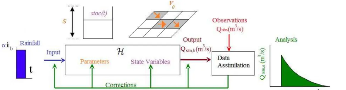
The conceptual hydrological model used in this study can be represented as a

non-10

linear operator, H, as in Fig. 6. This operator translates rainfall input data i_b into discharge data Q_sim, using model parameters (such as S and V₀) to solve ordinary differential equations for the state variables, stoc and P_b. Each of the parameters, inputs, state variables and outputs of this model is uncertain and could potentially be corrected with a DA algorithm using observed data. The output from the background

15

simulation (background discharge – before assimilation) is shown asQ_sim_,_b, the anal-ysis simulation (analanal-ysis discharge – after data assimilation) is shown as Q_sim_,_a, and the observations used to produce the analysis areQ_obs. In this study, the assimilation algorithm was applied to correct the radar rainfall,i_binput to the model using discharge observations. The correction, shown in Fig. 6, is a multiplicative coe_fficient of the

rain-20

fall intensity, denotedα, presented in Sect. 2.2.3. This coefficient is contained within the control vector,x₌(α).

Assuming that the errors in the model parameters and the observations follow a Gaussian distribution, the optimal value of the control vector is the analysis,xa, which minimizes the cost functionJ:

25

(18)

HESSD

9, 3527–3579, 2012

radar rainfall

E. Harader et al.

Title Page

Tables Figures

◭ ◮

Back Close

Full Screen / Esc

Discussion

P

a

per

|

Dis

cussion

P

a

per

|

Discussion

P

a

per

|

Discussio

n

P

a

per

|

The cost function, J expresses the difference between the control vector, x and its a priori value, xb (the background), and the di_fference between the control vector in the observation space and the observation vector, yo, weighted respectively by the background and observation error covariance matrices, B and R. The background control vector is selected asx_b₌(1) (no change to the input rainfall). The observation

5

vector gathers together the observed discharges during the flood event.

Bothxbandyoare considered to deviate from the “true” state of the system,xt. The difference between each of xb,xa and yo and the true state, xt are the background, analysis and observation errors denotedǫ_b,ǫ_a andǫ_o. These errors are assumed to be unbiased and uncorrelated.

10

In Eq. (19), the observation operatorH is non-linear as it represents the integration of the hydrological model for a given radar rainfall data set. As a consequence, J is non-quadratic and an incremental approach is used to approximate xa such that

∇J(xa)=0. The increment,δx, is defined as:

δx₌x−xb. (20)

15

The Jacobian matrix H of the observation operator H is expressed using the Taylor expansion computed around a reference vectorxref, initially chosen asxb:

H(xb₊δx) ≈ H(xb)+∂H

∂x|xb(δx). (21)

Using Eq. (21), Eq. (19) reads:

J_inc(δx)=δxTB−1δx₊(yo− H(xb)−Hδx)TR−1(yo− H(xb)−Hδx). (22)

20

Taking the gradient ofJ_incleads to,

∇J_inc(δx)=B−1δx−HTR−1(yo− H(xb)

| {z }

d

−Hδx), (23)

whered is the innovation vector. J_inc is at a minumum when ∇J_inc is null. By setting Eq. (23) equal to 0 and solving forδx, the following solution is generated:

δxa₌Kd (24)

(19)

HESSD

9, 3527–3579, 2012

radar rainfall

E. Harader et al.

Title Page

Tables Figures

◭ ◮

Back Close

Full Screen / Esc

Discussion

P

a

per

|

Dis

cussion

P

a

per

|

Discussion

P

a

per

|

Discussio

n

P

a

per

|

Using Eq. (20),δxais solved forxa:

xa₌xb₊Kd, (25)

wherexais the Kalman Filter analysis andKis the gain matrix described by,

K=BHT(HBHT+R)−1. (26)

The use of the Kalman Filter analysis equations relies on the hypothesis thatH(x) is

5

linear on [xa,xref], wherex_ais the minimum ofJ_inc, the quadratic approximation ofJ. To compensate for non-linearities in H(x), the outer loop process used in this study allows for the recalculation of the linear tangent,Hat the location of the analysis of the previous iteration(xa) in order to create a new quadratic approximation ofJ, as shown in Fig. 7.

10

The formulation of the Kalman Filter derived above presents several key simplifica-tions when compared to other work. The control vector, often used to correct model states, contains a single constant parameter that is applied to the model inputs, (α). If applicable in this case, the state vector would include (stoc_{i ,j}(t_k),P_b_{i ,j}(t_k)), wherei andjrepresent the x and y coordinates of each point andt_kis some time step, k. Since

15

the control vector contains onlyα and is assumed constant in time, its background er-ror covariance matrix is not propagated in time. The analysis is then determined over the entire assimilation window.

The background error is assumed to follow a Gaussian model and is described by its variance as the control vector is a scalar. The background error variance is set to 40 %

20

ofx_bsquared. The value of 40 % was determined by taking the average of|1−MFBi|,

thus relatingBto the average rainfall correction.

The observation errors are supposed uncorrelated, makingRa diagonal matrix. The observation error variance, σ_obs2, is chosen to be inversely proportional to the dis-charge value, thus favoring larger disdis-charge observations. A proportionality coefficient,

25

(20)

HESSD

9, 3527–3579, 2012

radar rainfall

E. Harader et al.

Title Page

Tables Figures

◭ ◮

Back Close

Full Screen / Esc

Discussion

P

a

per

|

Dis

cussion

P

a

per

|

Discussion

P

a

per

|

Discussio

n

P

a

per

|

assimilation window selected (reanalysis or forecast mode).

σ_obs_,i2₌max

(βobs Q_i )

2_,0.01

fori₌t_i:t_f. (27)

Rhas a lower bound of 0.01 m6s−2 and no upper bound. As the errors coming from each source of information are not precisely known, different values of the proportion-ality coefficient were considered as described in Sect. 5.1.

5

The data assimilation algorithm described above is applied in 2 modes: reanalysis and forecast. In reanalysis, all valid observations during the rainfall event are assimi-lated and in forecast, the assimilation window ends 3 h before the flood peak. Beyond this time, the model is integrated to provide a forecast of the event peak.

4 Initialisation and calibration of the model

10

The hydrological model contains several types of parameters: watershed constants which can be calibrated using batch calibration procedures, mathematical properties of the equations and one initial condition of the watershed,S, which must be calibrated separately for each event. The watershed constants and the initial condition are cal-ibrated by selecting the value which maximises the IE of the simulated discharge for

15

a given event. In the case ofS, the calibration process is finished at this stage, while batch parameters are averaged over all events. It should be noted that while the lan-guage “initialisation” is used here, S is a parameter in this data assimilation system and not a model state, thus it does not evolve during the event.

4.1 Calibration of model parameters

20

(21)

HESSD

9, 3527–3579, 2012

radar rainfall

E. Harader et al.

Title Page

Tables Figures

◭ ◮

Back Close

Full Screen / Esc

Discussion

P

a

per

|

Dis

cussion

P

a

per

|

Discussion

P

a

per

|

Discussio

n

P

a

per

|

either ground rainfall or high quality radar rainfall data and discharges were available. The drainage coe_fficient, d s, is a mathematical property of the hydrological model equal to the coefficient of the exponential recession limb of the hydrograph. This is a constant for all episodes. Since the diffusion time,K_m, is a function of both V₀ and K₀, many values of these two parameters can result in the same velocity distribution

5

at the watershed outlet. To avoid problems of equifinality,K₀ was set as a fixed value before calibratingV₀. The parametersV₀,w,d sandK₀were set as 1.3 m s−1, 101 mm, 0.28 d−1and 0.3 (dimensionless) respectively for all events.

4.2 Initialisation ofS

The soil moisture deficit at the start of the event, represented by the parameter, S,

10

must be calculated at the beginning of each event. In reanalysis mode, a posterioriS values, hereafter referred to asS_cal, were calibrated for each episode of the 19 radar rainfall episodes using an objective function which maximises the IE value for simula-tions forced with the MFB corrected radar rainfall in order to minimise the error in the parameterisation. In forecast mode, the event hydrograph is not known. As a

conse-15

quence, S must be estimated at the start of the event using known indicators of the soil hydric state at this time. For example, piezometric readings could be used to esti-mate the hydric state of the watershed in the morning if heavy rain is predicted for the evening. In this study, a calibration curve relatingS to indicators of the catchment wet-ness state is used to estimate a prioriS values for each episode from measurements

20

of aquifer piezometry or soil moisture indicators derived from surface models (Coustau et al., 2012). These estimatedS values are referred to asS_reg.

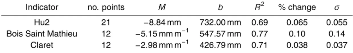
Using the historical record of discharge and rainfall from 1997–2008, calibration curves for S were developed using 3 catchment wetness state indicators: Hu2 (%), the piezometer located at Bois Saint Mathieu (m) and the piezometer located at Claret

25

(22)

HESSD

9, 3527–3579, 2012

radar rainfall

E. Harader et al.

Title Page

Tables Figures

◭ ◮

Back Close

Full Screen / Esc

Discussion

P

a

per

|

Dis

cussion

P

a

per

|

Discussion

P

a

per

|

Discussio

n

P

a

per

|

Segu´_ı, 2008) and estimates the % soil saturation at the root horizon. The measure-ments for each event are taken as the value of the indicator at 06:00 a.m. the day of the event. Hu2 data are available for 18 of the 19 events and piezometer data are available for 14 of the 19 events.

For each indicator, a regression of slopeM and y-interceptb was formed using the

5

indicator as the independant variable andS_cal as the dependant variable as shown in Table 2.R2is the coe_fficient of determination for the linear regression betweenS_caland the physical indicators. To validate each regression, split sample tests were performed. Each regression was performed using only the first half of the data available to con-struct a “historical period”; the S_reg values calculated using the validation regression

10

were then compared with theS_regvalues calculated using the regression for the entire record. The average and standard deviation of the % difference between these two S_reg values are presented in Table 2. The average % di_fference between S_reg for the validation curve andS_cal during the validation period was 0.22, 0.21 and 0.16 for Bois Saint Mathieu, Claret, and Hu2 respectively. When considering the difference between

15

S_reg and S_reg for the validation curve, the piezometer at Claret was the most robust indicator during validation. The validation curve S_reg values for Hu2 were closest to S_calduring the validation period.

TheS_regvalues calculated using the different regressions are shown in Table 3. The starred entries in this table represent events for which either indicator data was not

20

available or data assimilation was not preformed (October 2008). An analysis of the impact of errors in the parameterisation is presented in Sect. 5.3.1.

5 Application of data assimilation for the correction of radar rainfall

This section first explores the method of data assimilation applied in 2 modes: re-analysis and pseudo-forecast. In Sect. 5.2, the results of the rere-analysis mode are

25

(23)

HESSD

9, 3527–3579, 2012

radar rainfall

E. Harader et al.

Title Page

Tables Figures

◭ ◮

Back Close

Full Screen / Esc

Discussion

P

a

per

|

Dis

cussion

P

a

per

|

Discussion

P

a

per

|

Discussio

n

P

a

per

|

As mentioned in Sect. 3, the assimilation window ends 3 h before the flood peak in pseudo-forecast mode. This choice of assimilation window is intended to demonstrate the possible performance of the algorithm in a real-time forecasting environment, while acknowledging that the arrival time would not be known in this case. A complementary approach would be a sliding window, reflecting increased knowledge of the event as

5

time goes on.

5.1 Illustration of the data assimilation procedure

For the 19 radar rainfall events, the range of assimilated discharges is 15–300 m3s−1 for normal episodes and 2–40 m3s−1 for very small episodes (peak discharge less than or equal to 40 m3s−1). Very large discharges are unrealiable due to the use of

10

a rating curve to calculate the river stage-discharge relationship beyond 300 m3s−1. Small discharges are eliminated in order to better represent the flood behavior of the watershed. For each calculation of the analysis control vector in both analysis and forecast modes, 5 iterations of the outer loop method were used.

Episodes with notable double peaks (September 2002, October 2002, December 2002,

15

September 2005 and October 2008) were separated into single peaks prior to assimila-tion due to the inability of the hydrological model to properly represent multiple peaks in succession. Data assimilation was applied to all episodes in both forecast and reanaly-sis mode, with the exclusion of October 2008. The rising limb of this event takes place over a period of time less than three hours long, thus no discharge measurements are

20

assimilated in forecast mode.

To illustrate the procedure in the two different modes, the episode of November 2008 was selected. In renalysis mode, the soil moisture parameter, S_cal is 142 mm. β_obs is chosen to be 0.25 m6s−2 in order to reflect an almost complete confidence in the observations. As shown in Fig. 8, the IE is improved from−0.52 to 0.72 following

as-25

(24)

HESSD

9, 3527–3579, 2012

radar rainfall

E. Harader et al.

Title Page

Tables Figures

◭ ◮

Back Close

Full Screen / Esc

Discussion

P

a

per

|

Dis

cussion

P

a

per

|

Discussion

P

a

per

|

Discussio

n

P

a

per

|

blue and the corrected rainfall is in light blue with each bar the width of a 1 h timestep. This color scheme is conserved throughout the paper. In this case, α₌0.70 for the analysis, meaning that the optimal state of the rainfall is less than that predicted by the uncorrected radar data. This reduced rainfall then results in an analysis hydrograph that is less than the background hydrograph.

5

In forecast mode, observations are assimilated from the start of the event until 3 h before the peak discharge. This process is illustrated in Fig. 9 for the forecast mode of November 2008; the first analysis and the final result of the outer loop are shown. For this demonstration, S and β_obs were kept the same as those for the reanalysis mode. The first iterate of the outer loop (black) overestimates the correction to the

10

rainfall for a majority of the assimilation period. This overestimation is corrected with subsequent iterates. The first iterate has the best IE with 0.71 which is nearly equal to that of the reanalysis mode. However, this is not the optimal state for the assimilation period (up to 3 h before peak flow). Following new estimations of the Jacobian matrix,

H, at the analysis location, the final IE after all iterations of the outer loop is 0.62. The

15

finalα was 0.61, suggesting that the algorithm underestimates the rainfall in forecast mode. The analysis hydrograph (green curve) is still improved over the background hydrograph (pink curve), as it reduces the amount of rainfall; however, the reduction is overestimated when only the start of the episode is assimilated.

It should be noted that several modifications to the assimilation procedure are

neces-20

sary to optimally assimilate data in the forecast mode. First of all, an a priori estimation ofS (Sreg), as presented in Sect. 4, is required. Secondly, the observation error

co-variance must be adjusted to reflect representativeness errors due to the size of the assimilation window (only the start of the event is known). To account for increased errors in the observations,β_obs should be increased in the forecast mode. Trials using

25

(25)

HESSD

9, 3527–3579, 2012

radar rainfall

E. Harader et al.

Title Page

Tables Figures

◭ ◮

Back Close

Full Screen / Esc

Discussion

P

a

per

|

Dis

cussion

P

a

per

|

Discussion

P

a

per

|

Discussio

n

P

a

per

|

5.2 Reanalysis mode results

5.2.1 Impact of the rainfall correction

For the reanalysis mode, results are compared to the background state simulations and then to simulations with the MFB-corrected radar rainfall. Figure 10 presents the change in IE for the reanalysis compared with the background state for 19 episodes

5

with 7 additional peaks due to separation of multi-peak episodes. The IE values for simulations using uncorrected radar rainfall (the background simulation) are poor and in most cases are not of sufficient quality to reproduce the flood event. The qual-ity of the simulation is greatly improved following data assimilation and IE values are between 0.5 and 1 for a majority of episodes. The only degraded episode is that of

10

December 2003; this deterioration is related to the 300 m3s−1 upper assimilation limit described in Sect. 5.1 and is discussed in greater detail in Sect. 5.2.3.

5.2.2 Comparison of data assimilation to the MFB correction

A linear regression was performed between the MFB andα as shown in Fig. 11. The two quantities are expected to be related as they both represent corrections to the same

15

rainfall. If errors due to other sources are minimized (parameterisations, measurement errors for the gauges and discharge), the two corrective factors should tend towards the same value. The two quantities are well correlated with a R2 equal to 0.77. The slope, however, is 1.12, which suggests a systematic underestimation of rainfall by the MFB correction ifαis considered to be the optimal state.

20

The difference between the simulated discharges resulting from the rainfall corrected by the DA procedure and the MFB correction is presented in Fig. 12. The change in PH was calculated as PHMFB−PHα; positive results are thus increases in the positive

y-axis. 78 % of episodes showed an improved IE and 81 % of episodes showed an improved PH compared to the MFB correction. The average improvement in IE was

25

(26)

HESSD

9, 3527–3579, 2012

radar rainfall

E. Harader et al.

Title Page

Tables Figures

◭ ◮

Back Close

Full Screen / Esc

Discussion

P

a

per

|

Dis

cussion

P

a

per

|

Discussion

P

a

per

|

Discussio

n

P

a

per

|

value of 0). When deteriorations in the IE occured, they have the tendancy to be small, (−0.01 to−0.06). Deteriorations in the PH have a much larger range (₊0.02 to 0.21).

In most cases,αprovides improved results over the MFB correction. However, some of the improvement in the simulations withα when considering double peaks may be due to an increased time resolution. The MFB was calculated using rainfall over the

5

entire event, whereas the events were seperated into single peaks when usingα. The MFB is also calculated over a much larger spatial extent than that of the physical basin, leading perhaps to representativeness errors.

5.2.3 Limitations

The quality of the December 2003 simulation (Fig. 13a) was degraded following data

10

assimilation when compared to the background state. This is the result of a non-monotonic error in the discharge during the episode, as seen in Fig. 13b. Positive errors in the rising and descending limbs of the hydrograph result in an analysis state with a reduced rainfall. However, the sign of the error in the region near the peak is negative and this part of the hydrograph is not well-represented. To counteract this problem, the

15

upper limit of assimilated observations can be increased to include more observations at the hydrograph peak. The inclusion of these points increases the number of negative errors taken into account by the algorithm and results in an analysis which decreases rainfall less than when discharge observations are limited to less than 300 m3s−1.

5.3 Forecast mode results

20

5.3.1 Sources of uncertainty

In forecast mode, the efficacity of the DA algorithm is affected by both a lack of informa-tion about the event (representativeness errors) and a poor parameterisainforma-tion compared to the a posterioriS values (S_cal). In this study, representativeness errors refer to the fact that the start of the event may not be indicative of what comes later. For example,

(27)

HESSD

9, 3527–3579, 2012

radar rainfall

E. Harader et al.

Title Page

Tables Figures

◭ ◮

Back Close

Full Screen / Esc

Discussion

P

a

per

|

Dis

cussion

P

a

per

|

Discussion

P

a

per

|

Discussio

n

P

a

per

|

a gently sloped rising limb may then be followed by a large and quickly-rising peak flow. In this case, the algorithm would miss the peak region if it was to match observations at the start of the event as closely as possible. With regards to the parameterisation, S_cal requires a fully described event to be calculated, thus in forcast mode,S must be estimated by physical indicators of catchment wetness state at the start of an event

5

using the regression curves described in Sect. 4.2. To select the highest quality re-gression, the assimilation results for 3 different catchment wetness state indicators will be considered in Sect. 5.3.2.

To compare the effects of the two sources of uncertainty discussed above, IE and PH values were compared for simulations using analyses calculated in forecast mode

10

with (1) parameterisation using S_Hu2 (β_obs₌0.25 m6s−2) and (2) di_fferent values of the R matrix (βobs=0.25 m

6

s−2, 25 m6s−2 and 250 m6s−2) and S_cal. The range of β_obs values helps to estimate the uncertainty coming from the observations, while the comparison of the data assimilation results using S_Hu2 and S_cal gives an idea of the uncertainty resulting from the parameterisation.

15

Figure 14a presents a box plot of the change in IE for the 4 cases and Fig. 14b presents the results for the PH. The error in the parameterisation a_ffects the median, as seen by the decreased median for the simulations usingS_Hu2, while the represen-tativeness error affects the spread of the results. The quality of improvements possible in forecast mode is thus affected by the physical parameter selected to calculateS_reg

20

and the range of those improvements is controlled byβ_obs.

5.3.2 Results for 3 different soil moisture parameterizations

Figure 15 presents boxplots of the improvements to IE and PH values for the three differentSparameterizations. β_obsis selected as 250 m6s−2in order to limit the amount of confidence placed in the observations when the event is incompletely described (the

25