www.ocean-sci.net/11/195/2015/ doi:10.5194/os-11-195-2015
© Author(s) 2015. CC Attribution 3.0 License.
Argo data assimilation into HYCOM with an EnOI method in the
Atlantic Ocean
D. Mignac1,2, C. A. S. Tanajura2,3,4, A. N. Santana2, L. N. Lima2, and J. Xie5
1Graduate Program in Geophysics, Physics Institute and Geosciences Institute, Federal University of Bahia, Salvador, Brazil 2Oceanographic Modeling and Observation Network, Center for Research in Geophysics and Geology,
Federal University of Bahia, Salvador, Brazil
3Physics Institute, Federal University of Bahia, Salvador, Brazil
4Ocean Sciences Department, University of California, Santa Cruz, CA, USA 5Institute of Atmospheric Physics, Chinese Academy of Sciences, Beijing, China Correspondence to:D. Mignac ([email protected])
Received: 8 April 2014 – Published in Ocean Sci. Discuss.: 2 July 2014
Revised: 18 December 2014 – Accepted: 8 January 2015 – Published: 11 February 2015
Abstract. An ocean data assimilation system to assimilate Argo temperature (T) and salinity (S) profiles into the HY-brid Coordinate Ocean Model (HYCOM) was constructed, implemented and evaluated for the first time in the Atlantic Ocean (78◦S to 50◦N and 98◦W to 20◦E). The system is based on the ensemble optimal interpolation (EnOI) algo-rithm proposed by Xie and Zhu (2010), especially made to deal with the hybrid nature of the HYCOM vertical coor-dinate system with multiple steps. The Argo T–S profiles were projected to the model vertical space to create pseudo-observed layer thicknesses (1pobs), which correspond to the model target densities. The first step was to assimilate1pobs considering the sub-state vector composed by the model layer thickness (1p) and the baroclinic velocity components. After that, T andS were assimilated separately. Finally,T
was diagnosed below the mixed layer to preserve the density of the model isopycnal layers. Five experiments were per-formed from 1 January 2010 to 31 December 2012: a control run without assimilation, and four assimilation runs consid-ering the different vertical localizations ofT,Sand1p. The assimilation experiments were able to significantly improve the thermohaline structure produced by the control run. They reduced the root mean square deviation (RMSD) ofT andS
calculated with respect to Argo independent data in 34 and 44 %, respectively, in comparison to the control run. In some regions, such as the western North Atlantic, substantial cor-rections in the 20◦C isotherm depth and the upper ocean heat content towards climatological states were achieved.
The runs with a vertical localization of1pshowed positive impacts in the correction of the thermohaline structure and reduced the RMSD of T (S) from 0.993◦C (0.149 psu) to 0.905◦C (0.138 psu) for the whole domain with respect to the other assimilation runs.
1 Introduction
analyses for climate diagnostics studies and they contribute to a better understanding of the physical mechanisms that are responsible for the ocean variability. For example, the depth of the mixed layer and the heat content can be better repre-sented by analyses than by model simulations without assim-ilation (Carton and Giese, 2008).
A major obstacle in ocean data assimilation is the rel-atively small volume of observed ocean data available for assimilation and validation. Most of the spatial and high-frequency temporal variability from the ocean surface is ac-quired by satellite measurements such as the sea surface height (SSH) and sea surface temperature (SST). However, these observations are available for only a few decades and they are insufficient to determine the sub-surface variability (Ezer and Mellor, 1994; Chassignet et al., 2006). Therefore, the implementation of the Argo network with more than 3300 profilers freely reporting temperature and salinity data down to 2000 m has transformed the in situ ocean observing system in the new millennium (Schiller and Brassington, 2011). For the first time it is possible to have continuous measurements of the temperature, salinity and velocity of the upper ocean which makes the Argo network indispensable for any global or regional data assimilation system (Chassignet et al., 2007; Oke et al., 2008; Xie and Zhu, 2010). For example, Oke and Schiller (2007) showed that the assimilation of SST and SSH should be complemented with Argo profiles since the assimi-lation of this component plays a crucial role in improving the model thermohaline state, especially for salinity.
Among all data assimilation methods, the ensemble-based methods use a set of different model states to estimate the model errors (Evensen, 2003; Oke et al., 2005). One widely used is the ensemble optimal interpolation (EnOI) (Oke et al., 2005) in which the ensemble members are derived from an existing model run. This reduces the computational cost of the assimilation and makes this method suitable for oper-ational purposes. It is already verified that the EnOI is able to effectively constrain the model towards observations. For instance, it was successfully applied to assimilate Argo data in the Pacific Ocean (Xie and Zhu, 2010), sea level anomaly (SLA) data in the South China Sea (Xie et al., 2011) and in the Gulf of Mexico (Counillon and Bertino, 2009), and SLA, SST and Argo data in the Australian region (Oke et al., 2008) and in the Indo-Pacific Ocean (Yan et al., 2010).
Considering the importance of the model in the construc-tion of the analysis, several state-of-the-art, publically avail-able ocean circulation models should be evaluated in order to develop an operational ocean forecasting system with data assimilation. One choice is the HYbrid Coordinate Ocean Model (HYCOM). It is formulated in terms of target densi-ties and employs a hybrid vertical coordinate system to com-bine the best features of each vertical coordinate in specific oceanic regions (Bleck, 2002). The model has fixed z-levels to better represent the mixed layer, isopycnal layers to dis-cretize the deep stratified ocean andσ-levels to better repro-duce the bathymetry in shallow areas. Because of the hybrid
nature of the model, the best way to assimilate vertical pro-file data into HYCOM is still an open question. A choice of the model prognostic variables should be made a priori since only two of the three state variables – temperature, salinity and potential density – are independent. Furthermore, the layer thickness, which is a key model variable, varies spa-tially and temporally according to the evolution of tempera-ture, salinity and density.
Taking into account these characteristics, Thacker and Es-enkov (2002; hereafter TE) proposed a method to assimilate expendable bathythermographic (XBT) data into HYCOM with a three-dimensional variational scheme (3-D Var). In this work, the XBT profiles are converted into observed layer thicknesses that respect the target densities of each model layer, and the temperature and salinity of the XBTs are pro-jected to each observed layer thickness. Xie and Zhu (2010; hereafter XZ) used an EnOI scheme to assimilate Argo data, and showed that the TE approach produced significant im-provements in relation to simpler schemes, in which the in-novation is calculated in the observational space.
Very little has been published to evaluate the impact of in situ profile data assimilation into HYCOM with a focus on the Atlantic Ocean (e.g., Thacker et al., 2004; Belyaev et al., 2012). In the present work, a data assimilation sys-tem for HYCOM was constructed, implemented and real-ized for the Atlantic Ocean for the first time. The data as-similation algorithm follows the EnOI scheme suggested by XZ very closely. The present system was developed within the Brazilian Oceanographic Modeling and Observation Net-work (REMO) to be a component of an operational ocean forecasting system for the Atlantic Ocean (www.rederemo. org) (Tanajura and Belyaev, 2009; Lima et al., 2013; Tanajura et al., 2013). In this paper, the focus is on the impact of Argo data assimilation over the Atlantic Ocean and on a sensitiv-ity study of the analysis run, considering different vertical localizations of the model error co-variance matrix involv-ing temperature, salinity and especially the layer thickness. The REMO forecasting system uses a nested model approach based on HYCOM. The present work deals with the con-struction of large-scale analyses over almost the whole At-lantic Ocean. This domain was conceived and configured to provide reasonable boundary conditions to higher-resolution grids of greater interest to REMO over the South Atlantic. In the near future, the present data assimilation methodol-ogy will be used in the Atlantic domain, and in the higher-resolution grids over the Metarea V (from 35.5◦S to 7◦N,
west of 20◦W to Brazil) and sub-regions off the Brazilian
coast of particular interest to the Brazilian Navy and the ac-tive petroleum industry located there.
2 HYCOM and its configuration
HYCOM is a primitive equation general circulation model, which has evolved from the Miami Isopycnic Coordinate Ocean Model (MICOM) (Bleck and Smith, 1990). The main advantage of the isopycnal coordinate is its ability to main-tain the properties of water masses which do not commu-nicate directly with the mixed layer. In HYCOM, with the advection of layer thicknesses by the continuity equation, the isopycnal coordinates smoothly transform into the z -coordinate in the weakly stratified upper ocean mixed layer and into the terrain-following σ-coordinate in the shallow water regions (Bleck, 2002; Chassignet et al., 2007). The freedom to adjust the vertical spacing of the coordinate sur-faces in HYCOM simplifies the numerical implementation of several physical processes, such as turbulence in the mixed layer, detrainment and convective adjustment. Also, the ca-pability of assigning additional coordinate surfaces to the oceanic mixed layer in HYCOM allows the option of im-plementing sophisticated vertical mixing turbulence closure schemes (Halliwell, 2004). Hence, HYCOM is considered to be a suitable model for operational ocean forecasting sys-tems and climate studies (Chassignet et al., 2007, 2009). In this work, the version 2.2.14 of HYCOM was used.
The model grid in the present configuration has 760×480 horizontal grid points, with a spatial resolution of 0.25◦, which remains constant in longitude, but varies in latitude attaining higher resolution towards the poles. The computa-tional model domain covered almost all the Atlantic Ocean from 78◦S to 50◦N and from 100◦W to 20◦E, excluding
the Pacific Ocean, the Mediterranean Sea and the North At-lantic subpolar region. The choice for the northern limit at 50◦N was based on two facts. First, the surface currents
are primarily zonal at this latitude (Gabioux et al., 2013). Second, the purpose of this grid is to provide reasonable boundary conditions to higher-resolution grids that will soon be configured along the Brazilian coast, which is the area of main interest to REMO and far away from the northern boundary. On the lateral boundaries, relaxation to monthly climatological temperature and salinity from Levitus (1982) was applied considering the outermost 10 grid cells and the timescale of 30 days. This approach attempts to preserve cli-matological shear through geostrophic adjustment and has been successfully used in previous works (e.g., Paiva and Chassignet, 2001; Gabioux et al., 2013). Constant barotropic volume fluxes were imposed: zero flux in the north, eastward flux of 110 Sv in the Drake Passage, westward flux of 10 Sv in 12 grid points adjacent to South Africa along 20◦E, and
eastward flux of 120 Sv further south to Antarctica.
The model was configured to use surface pressure as ref-erence for potential density, aiming for improved represen-tation of near-surface fields, at the cost of not representing accurately the Antarctic Bottom Water (Chassignet et al., 2003). The vertical domain was discretized in 21 vertical lay-ers. The chosen target potential densities were 19.50, 20.25,
21.00, 21.75, 22.50, 23.25, 24.00, 24.70, 25.28, 25.77, 26.18, 26.52, 26.80, 27.03, 27.22, 27.38, 27.52, 27.64, 27.74, 27.82 and 27.88. To obtain the volumetric density in kg m−3, 1000 should be added to each target density. The first layers have a few light target density values that ensure a minimum of three fixed-depth layers near the surface of the ocean.
The vertical mixing scheme is the K-profile parameteri-zation (KPP) (Large et al., 1994). The model bathymetry was interpolated from the Earth Topography 1 (ETOPO1) with 1 min resolution. The model was initialized from the state of rest with climatological thermohaline structure, and a 30-year spin-up was performed using monthly climato-logical forcing fields from the Comprehensive Ocean and Atmosphere data set (COADS) (Woodruff et al., 1987). Then, from January 1995 to December 2009, the model was forced on the ocean surface with 6-hourly atmospheric re-analysis version 1 by the National Centers for Environmen-tal Prediction/National Centers for Atmospheric Research (NCEP/NCAR) (Kalnay et al., 1996), including precipita-tion, wind speed at 10 m, short- and long-wave radiation fluxes at the surface, air temperature and humidity at 2 m. The result of this simulation was used as the initial condi-tion for the Argo data assimilacondi-tion experiments starting on 1 January 2010.
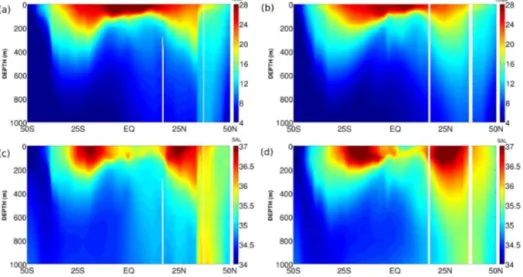
Figure 1 shows the mean state of temperature and salinity simulated by HYCOM from 1 January 1997 to 31 December 2008 and its comparison with the World Ocean Atlas 2013 Climatology (WOA13) (Boyer and Mishonov, 2013) along 25◦W for the upper 1000 m. WOA13 climatology shown in Fig. 1 spans the period from 1995 to 2012. In general, the pattern of the simulated temperature and salinity is similar to the WOA13 climatology, particularly in the South Atlantic, which is the main target area for REMO. In the North At-lantic large differences are seen between 25 and 50◦N
Figure 1.Mean temperature (◦C) and salinity (psu) in the upper 1000 m along 25◦W for(a)averaged simulated temperature from January 1997 to December 2008,(b)climatological temperature from WOA13,(c)averaged simulated salinity from January 1997 to December 2008, and(d)climatological salinity from WOA13.
3 The data assimilation scheme
The analysis (Xa) according to the EnOI scheme is given by the formula (Evensen, 2003)
Xa=Xb+K(Y−HXb), (1) whereXb∈RN is the model background state or the prior, K is the gain matrix,Y is the vector of observations, Y ∈
RNOBS, and HXb is the projection of the prior onto the observational space by the observational operator H. The term(Y−HXb)is called the innovation vector and the term K(Y−HXb)is the analysis increment. The gain matrixKis calculated from the equation
K=α(σ◦B)HT[αH(σ◦B)HT+R]−1, (2) whereBis the co-variance matrix of the model errors andR is the diagonal variance matrix of the observational error. The termα∈(0,1]is a scalar that can tune the magnitude of the analysis increment and σ denotes the localization operator applied overBby a Schur product represented by the symbol
◦. Equation (2) is used by many data assimilation schemes such as the optimal interpolation, the ensemble Kalman fil-ter (EnKF) or the EnOI. In the EnOI scheme,Bis estimated from the equation
B=
A′A′T
(M−1), (3)
where A′= [A′1
A′2, . . ., A′M], A′k=(Xk− 1
M
PM
m=1Xm), Xk∈RNis the model state vector of thekth ensemble mem-ber withkvarying from 1 toM, andM=132 is the number of ensemble members used in all assimilation steps in this study. This ensemble of model anomalies can be taken from
a long-term model run (Evensen, 2003) or a spin-up run (Oke et al., 2008) in order to capture the model variability at cer-tain scales. Thus, even being stationary in time, this ensemble of model anomalies allows for the description of the spatial correlations and the anisotropic nature of ocean circulation, keeping the analysis dynamically consistent and substantially reducing the computational cost. Details on how theBmatrix was calculated here regarding the high-frequency variability of the model are described below.
3.1 Calculation of the innovation vector
Figure 2.Profile of potential temperature (◦C), salinity (psu) and potential density (kg m−3) from an Argo float located at 4.04◦N and 23◦W on 1 January 2010 plotted against its approximation for HYCOM as layer averages. The model target density is indicated by the solid black vertical lines.
by an equation of state for seawater (Brydon et al., 1999). The estimated surface density from the Argo profile is com-pared to the top layer target density to decide whether any sufficiently low-density water was observed. If not, the min-imum thickness is assigned to the layer and the procedure is repeated for the layer below. Once water with the target density is encountered, the remainder of the potential density profile can be partitioned and the layer averages will corre-spond to the model target densities down to the maximum depth of the Argo profile.
Figure 2 shows the vertical profiles of potential temper-ature, salinity and potential density at z-levels and the new synthetic observations defined at model layers for an Argo float located at 4.04◦N and 23◦W on 1 January 2010. In Fig. 2, each1pobsrespects the target densities of the model as soon as the first target density is found in the potential density profile of the Argo data. Also, the averages for all the observational variables are computed for each layer, as shown by the discretized profiles of potential temperature and salinity in the model layers. The step functions of T,
Sand1pobsare the data that will be actually assimilated by the EnOI scheme.
3.2 The modified EnOI to assimilate profile data into HYCOM
After the observation is defined in the HYCOM layers, the observed layer thicknesses are assimilated in a first step by Eqs. (1) and (2), and the analysis update is carried out for the model control state vector (1pi,Ui,Vi); i=1, . . ., nz,
where1pi,Uiand Viare the layer thicknesses and the
baro-clinic velocity components, respectively, defined at the nz model layers for a single time step. To avoid the analyzed layer thicknesses occasionally becoming negative, a
compu-tationally efficient scheme based on Sakov et al. (2012) is used. If the thickness of a layer becomes negative, it is reset to zero and the thickness deficit is added to the neighboring layers. The layers are traversed twice, once from top to bot-tom, and a second time from bottom to top. Finally, the sum of the layer thicknesses should be equal to the initial bottom pressure (or local depth).
In the next step, temperature and salinity are assimilated separately and in a univariate way also according to Eqs. (1) and (2), but now with the previously adjusted layer thick-nesses. Finally,T orSis diagnosed below the mixed layer by the seawater equation of state. According to TE, “within the context of HYCOM, when correcting temperature, it is nec-essary to decide whether to move interfaces, keeping poten-tial densities of the layers unchanged, or to correct the densi-ties, leaving the interfaces unchanged”. Therefore, when the assimilation of layer thicknesses is performed, the potential density should be kept constant in the ocean simulated with isopycnal coordinates. Considering that most of theT cor-rections in the experiments of XZ were due to changes in the layer thicknesses by the assimilation of1pobs,T was chosen to be diagnosed below the mixed layer in the present work, instead ofS.
3.3 Generation of a running ensemble
Many authors have shown how sensitive the EnOI and EnKF schemes are to the ensemble size (Mitchell et al., 2002; Evensen, 2003; Oke et al., 2007). In the EnOI scheme, the propagation of the observational information is highly de-pendent on the size and the quality of the ensemble, be-cause the final analysis can be regarded as a combination of the ensemble anomalies whose relative weight is determined by the co-variances. In this work, 132 ensemble members were used. They were selected from the model free run for each assimilation day, regarding the intra-seasonal variabil-ity and the high-frequency model dynamics. This number of ensemble members was chosen after a few sensitivity experi-ments considering a reasonable representation of the model’s anomalies without high computational cost, and is in agree-ment with the numbers used in recent works (e.g., Counillon and Bertino, 2009; Xie and Zhu, 2010; Xie et al., 2011).
3.4 Localization
The localization technique is a feasible solution to reduce the effect of the sampling error in the ensemble-based meth-ods, especially when the ensemble size is small (Hamill et al., 2001; Oke et al., 2007). The significance range of a mea-surement is a critical question in assimilation. In the present case, it should be unreasonable that a measurement in the Gulf Stream contributes to resolving the mesoscale features of the circulation of the Brazil Current. Therefore, the lo-calization aims to delete long-distance correlations that may appear in the gain matrix and to limit the influence of a single observation by the Kalman update equation within a fixed re-gion around the observation location. However, a drawback of the localization is that it can breakdown the geostrophic balance. Oke et al. (2007) showed that localization conserves the geostrophic balance when the radius of the localization is equal to or larger than the radius of decorrelation, which is the scale in which the correlations become negligible.
For many EnKF and EnOI schemes, localization is only applied in the horizontal direction (Oke et al., 2008; Sakov et al., 2012). However, some works have already investigated the vertical localization and its impact on the analysis, such as in XZ. They presented a vertical localization scheme forT
andSwhen assimilating Argo profiles into HYCOM. Here, localization in the vertical direction is also investigated, but differently from XZ, as the focus is on1p.
The operatorσ◦in Eq. (2) defines the implementation of the localization by a Schur product, i.e., a product between elements with the same index in the arrays. The notationσ◦B denotes the Schur product of a correlation matrixσ with the Bmatrix, and this approach is used in many works (Oke et al., 2007, 2008; Xie and Zhu, 2010). Here, the localization operator is separated into a horizontal component(σh)and a vertical component(σv), and it is defined asσ=σhσv. 3.4.1 Horizontal localization
In order to define the horizontal correlation matrixσh, a fifth-order function is used as in Gaspari and Cohn (1999):
σh Iij, L= (4)
−1 4 Iij L 5 +1 2 Iij L 4 +5 8 Iij L 3 −5 3 Iij L 2
+1, 0≤Iij≤L 1 12 Iij L 5 −1 2 Iij L 4 +5 8 Iij L 3 +5 3 Iij L 2
−5IijL+4−2 3
Iij
L
−1
, L < Iij≤2L
0, Iij>2L
In this function,Iijis defined as the Euclidean distance
be-tween any two arbitrary points in the horizontal space andL
is the horizontal scale of influence defined as 150 km for all the assimilated variables. It is similar to a Gaussian function in physical space but more compact. The correlation function σhforces the model error co-variance matrixB to decrease to zero when Iij reaches 300 km. Thus, the radius of
local-ization is defined as 300 km.
The horizontal scale of influence was chosen to be 150 km because this number roughly matches the scales of boundary
currents (Ezer and Mellor, 1994; Carton and Giese, 2008). Since the present work was the first REMO effort to im-plement an EnOI scheme to assimilate Argo data into HY-COM, the horizontal scale of influence was fixed for the en-tire model domain and for all depths. In this case, the choice of 150 km was conservative in order to avoid capturing co-variances that could damage the analysis in high-variability regions, such as the Gulf Stream and the Brazil–Malvinas Confluence.
3.4.2 Vertical localization
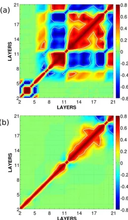
Concerning the vertical localization, XZ found considerable off-diagonal correlations for temperature and salinity be-tween different HYCOM layers. However, there was no sig-nificant impact in the analysis when those co-variances were filtered and no significant differences in the experiments with and without vertical localization were reported. However, in the present work the vertical localization of co-variances be-tween the layer thicknesses was investigated. They showed considerable off-diagonal correlations of above 0.4 or below
−0.4 from the seventh layer to the bottom (Fig. 3). In the for-mulation of the vertical localization operator, the vertical dis-tance between the layers was measured by the water column stratification, rather than by the Euclidian distance. Thus, in order to define the correlation matrixσv, the following func-tion was used:
σv
(i,j )=exp
h
−(1ρ(i,j )/Lρ)2 i
, (5)
where1ρ(i,j )is the density difference between the HYCOM
layersi andj, andLρ is a vertical-scale factor defined as
0.5 kg m−3according to XZ. As shown by Fig. 3, when ap-plying the vertical localization, the elements a few entries away from the diagonal in the co-variance matrix are almost canceled, but the correlations between the adjacent layers re-main.
3.5 Observational errors
Since the observations that are actually assimilated are de-fined in the model vertical space, the observational errors of
T andSin the model layers are calculated as a function of the depthDin meters, respectively, as in XZ:
SDT(D)=0.05+0.45 exp(−0.002D), (6) SDS(D)=0.02+0.10 exp(−0.008D). (7) The standard deviations of the observational errors ofT
vary in the vertical from 0.5◦C on the surface to 0.05◦C in
the deep ocean. ForS, they vary from 0.12 to 0.02 psu. Ac-cording to Eqs. (6) and (7), the observational errors are as-sumed Gaussian with zero mean and uncorrelated.
Figure 3.Vertical correlations of layer thickness between different layers at the location of an Argo float (69.95◦W and 30.14◦N) in the model domain:(a)calculated directly from the model ensembles (M=132) and(b)after applying the vertical localization of layer thickness according to Eq. (5) andLρ defined as 0.5 kg m−3. The
white lines denote correlations above 0.4 and below−0.4.
is assigned to the minimum layer thickness allowed by the model configuration, and the standard deviation is defined as 0.051pk, where1pkrepresents the layer thickness at thekth
layer calculated from the observed profiles. In the isopycnal layers, the standard deviation is defined by the formula
SD(1pk)=max (8)
0.5δpk,max
0.051pk, 1pk
0.05+(0.5−0.05)sdσ (k)
SDσ (k)
,
whereδpk is the minimum layer thickness specified by the
model configuration for the kth layer, sdσ (k) is the
mini-mum standard deviation of the potential density defined as 0.001 kg m−3, and SDσ (k)is the standard deviation of the
po-tential density from observations. The latter should be small when the potential density from the observed layer thickness has values close to its target density.
4 Assimilation experiments 4.1 Argo data and quality control
The Argo data employed in the assimilation were collected from a global data center (available at: ftp://ftp.ifremer. fr/ifremer/argo/geo/atlantic_ocean/). All those observations were required to step into a data quality control (QC) pro-cedure, which is an essential part to any oceanic data assim-ilation system since spurious data can compromise the anal-ysis quality and introduce artificial trends in the assimilation results (Yan and Zhu, 2010). The QC used in this work was both developed by REMO together with the Brazilian Navy and tests the date, the location and the temperature and salin-ity of each Argo profile previously collected. The validation ofT andS profiles was made according to all criteria and references established by the Global Temperature and Salin-ity Pilot Program from the Intergovernmental Oceanographic Commission (IOC, 1990) and from the database of the Na-tional Oceanographic Data Center (NODC).
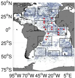
From January 2010 to December 2012, 47 999 valid Argo profiles were assimilated into HYCOM in the Atlantic Ocean. These profilers covered almost the entire model do-main, and were especially dense in the North Atlantic, as shown in Fig. 4.
4.2 Configuration and evaluation of the assimilation experiments
Five integrations were performed from 1 January 2010 to 31 December 2012 to evaluate the impact of the Argo data assimilation and the vertical localization in the correction of the ocean state and circulation. The first one was a control run without assimilation (CTL). The other runs were assimilation runs, namely, (i) assimilation without vertical localization (ASSIM), (ii) assimilation with vertical localization of layer thickness (VL_DP), (iii) assimilation with vertical localiza-tion of temperature and salinity (VL_TS) and (iv) assimila-tion with vertical localizaassimila-tion of all the assimilated variables (VL_DPTS). In all experiments with data assimilation, a 3-day observational window was considered in order to select all the valid profiles collected 3 days before the assimilation day. The interval between each assimilation step was also 3 days and the scalarαin Eq. (2) was defined as 0.3.
Figure 4.Locations of the 47 999 valid Argo profiles (blue dots) as-similated and also used to validate the prior state of each experiment from 2010 to 2012 in the model domain (100◦W–20◦E, 78◦S– 50◦N), which excludes the Pacific Ocean, the Mediterranean Sea, and the North Atlantic subpolar region. The 16 fixed moorings from PIRATA used in the experiment’s validation are represented by red dots. The numbers of valid Argo profiles in the 12 sub-regions (a–l) were 3085, 2352, 2522, 540, 1463, 2750, 2475, 1849, 1560, 1597, 2536 and 3067.
to the evaluation of forecasts. Moreover, 16 fixed moorings from the Prediction and Research Moored Array in the Tropi-cal Atlantic (PIRATA) were used as another independent data set for validation. Their locations are represented by red dots in Fig. 4. Also, the domain was split into 12 sub-regions from a to l, as shown in Fig. 4, in order to evaluate the regional impact of the assimilation. These sub-regions and their coor-dinates were selected taking into account the spatial distribu-tion of the surface mean kinetic energy and the mean stan-dard deviations of SSH, SST and sea surface salinity (SSS) from 1997 to 2008. The numbers of Argo profiles assimi-lated in the experiments in the 12 sub-regions a–l were 3085, 2352, 2522, 540, 1463, 2750, 2475, 1849, 1560, 1597, 2536 and 3067.
Outputs from the HYCOM Navy Coupled Ocean Data Assimilation (HYCOM+NCODA) (Chassignet et al., 2007, 2009) system available in z-levels and fields from the Ocean Surface Current Analyses Real Time (OSCAR) (Johnson et al., 2007) were employed to compare the velocity fields pro-duced by the assimilation runs. Also, WOA13 climatology for the period from 2005 to 2012 was used to evaluate the mean state of T, S and heat content of the upper 300 m (HC300) in all experiments. In this period, WOA13 includes the global coverage of Argo floats to compose the climato-logical gridded fields ofT andSin 1/4◦of spatial resolution.
5 Results
5.1 Comparison of mean states
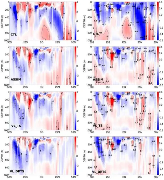
The first comparison is conducted with the WOA13 climatol-ogy along 25◦W for the upper 1000 m (Fig. 5). It was already verified that the free model run mean from 1997 to 2008 showed substantial differences with respect to the WOA13 climatology (Fig. 1). According to Chen et al. (2000), ocean circulation models can naturally present large and systematic biases inT andS due to their initialization and configura-tion. This is also shown by the control run, particularly in the North Atlantic. As mentioned before, to simulate the MW in the Atlantic, relaxation ofT andSin the boundary condition is imposed without mass flux. Moreover, the resolution of 1/4◦could also be a limitation to accurately solve the Gulf
Stream and its associated dynamics in the mid-latitudes of the North Atlantic (Hulburt and Hogan, 2000). The main pur-pose of this grid is to provide boundary conditions for higher-resolution grids focusing on the Metarea V. However, even with these limitations, the assimilation schemes are able to substantially reduce these differences and correct the ocean state towards WOA13. For example, the positive temperature bias up to 3◦C and the negative salinity bias up to 0.4 psu in the upper 300 m of the control run are not produced in any assimilation run. Moreover, all the discrepancies found in the MW are remarkably diminished in the data assimilation runs, which are able to decrease the differences in 0.6 psu and more than 2◦C towards WOA13 between 20 and 40◦N in the sub-surface, especially below 400 m. This correction is very effective in the VL_DP and VL_DPTS runs, which adopt the vertical localization of1p. The VL_DPTS run is able to more efficiently improve the mean T andS states in the North Atlantic along the entire water column by fur-ther reducing the differences of 1◦C and 0.1 psu found in the other assimilation runs with respect to WOA13. Also, at 300 m near 25◦S, only the VL_DPTS run decreases the dif-ferences towards WOA13 from more than 3 to almost 1◦C, while the ASSIM and VL_TS runs are not able to reduce these differences with respect to the control run. But, south of 30◦S, the improvements ofT andSin the VL_DPTS are considerably smaller than those obtained by the other assim-ilation runs.
Near 50◦S, the control run does not well represent the for-mation of the Antarctic Intermediate Water Mass (AAIW). The experiments with data assimilation can correct the neg-ative biases shown by the control run by up to 2◦C and
Figure 5.The model mean minus WOA13 along 25◦W in the upper 1000 m for temperature (◦C) on the left and salinity (psu) on the right from 1 January 2010 to 31 December 2012 according to the CTL run and the prior state of the ASSIM, VL_TS and VL_DPTS runs.
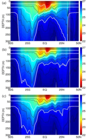
In order to investigate how stratification was modified by Argo data assimilation in the upper 300 m, Fig. 6 shows the meridional section along 25◦W of the mean potential density
and the position of the layers interfaces for the experiments CTL, ASSIM and VL_DPTS. In general, as already shown in Fig. 5, the assimilation runs tend to decrease the temper-ature and increase the salinity in the upper 300 m, driving the model towards WOA13. This is associated with a gen-eral increase of the mean potential density in the sub-surface in all the assimilation experiments, especially between 30◦S and 30◦N. This increase of the potential density can reach more than 0.5 kg m−3 near the equator and in the subtrop-ical gyres. According to Bleck (2002), the implementation of the isopycnal vertical coordinate in HYCOM follows the theoretical formulation that each isopycnal layer will move to be as close as possible to its target density. Therefore, in the assimilation experiments the deeper layers will move towards the surface to encompass the density increase pro-duced by theT andSincrements and satisfy their target
den-sities. For example, near the equator and in the subtropical gyre of the South Atlantic, there is a displacement of 25 m or more of the deeper layer interfaces towards the surface. In the North Atlantic, this displacement is even larger and it can reach 150 m, as can be seen by the behavior of the lower-most white dashed line in Fig. 6 that represents the interface between the 11th and 12th layer. Large et al. (1997) showed that the warm temperature bias near the equator is a common feature of coarse-resolution models and it is related to weak zonal currents and weak zonal slopes of the isotherms. How-ever, all the data assimilation experiments are able to force the present low-resolution model to stack the layer interfaces in the upper 300 m and correct the model bias of temperature and salinity not only at the equator but also at all latitudes, especially between 30◦S and 30◦N.
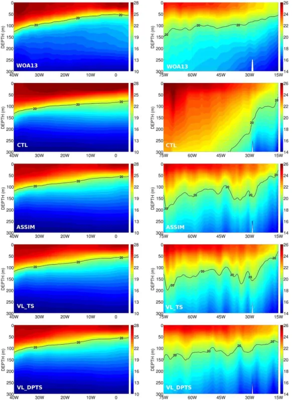
The depth of the 20◦C isotherm is also evaluated for the experiments and the WOA13 climatology in two longitudi-nal sections, one along the equator and the other along 30◦N
equator is about 120 m in the west and it gets shallower in the east with a value of almost 50 m. The control run is clearly warmer than WOA13 in the upper ocean with temperatures higher than 28◦C in the first 100 m, so that the position of
20◦C isotherm is deeper, especially in the east of the section with values close to 100 m. All the assimilation experiments reduce the warm bias in the upper ocean, and the depth of 20◦C isotherm is lifted to a shallower position in much bet-ter agreement with the WOA13 climatology. In the North At-lantic, the control run has an even stronger bias of more than 4◦C in the upper 300 m. Hence, the depth of 20◦C isotherm of the control run is deeper than WOA13, attaining more than 300 m in the west of the section. Again, the experiments with data assimilation are able to significantly reduce the warm bias by moving the position of the 20◦C isotherm more than
150 m towards the surface. This agrees very well with the large displacement of the layer interfaces in the North At-lantic shown in Fig. 6, and also with the WOA13 climatol-ogy. Along 30◦N, between 75 and 65◦W and between 40
and 25◦W, the experiment VL_DPTS is able to bring the 20◦C isotherm up to 50 m closer to the surface in comparison with the other runs without the vertical localization of layer thickness. On the other hand, the experiment VL_DPTS is the only assimilation experiment that does not represent very well the upwelling in the east margin of the Atlantic Ocean at 30◦N in Fig. 7. Probably, this is because there is a strong ver-tical correlation among several model layers in the upwelling region that is not considered by the vertical localization of layer thickness in the VL_DPTS run. Similar behavior was observed in the region of AAIW formation shown in Fig. 5.
To further assess the impact of the assimilation in the up-per ocean thermal structure, the spatial distribution of the HC300 between 50◦S and 50◦N is presented in Fig. 8 for
the WOA13 together with the differences (model mean mi-nus WOA13) for each run. In general, the control run has a larger HC300 in comparison with the WOA13 climatol-ogy. Vast areas of the North and South Atlantic have more than 50 MJ m−2of HC300 excess over the climatology. The largest differences are attained in the Gulf Stream region (about 400 MJ m−2), since it is misplaced northward with re-spect to observations, and in the southwest Atlantic around 40◦S, associated with a misrepresentation of the Brazil– Malvinas Confluence. When Argo data are assimilated, the model temperature is constrained towards WOA13 and there is a strong impact on the HC300. All the assimilation ex-periments decrease the HC300 difference with respect to WOA13 by more than 150 MJ m−2 for large areas of the subtropical North Atlantic and 50 MJ m−2in the equatorial and South Atlantic. However, large differences still remain in the simulated Gulf Stream region. No Argo data were avail-able in this shelf region – to the north of the observed Gulf Stream – to constrain the model (Fig. 4); therefore, the as-similation runs could not correct this discrepancy. Also, no SST and SLA were assimilated and the assimilation of Argo
Figure 6.Potential density (kg m−3) and the position of the layer interfaces along 25◦W in the upper 300 m for the(a)CTL run and the prior state of the(b)ASSIM and(c)VL_DPTS runs from 1 Jan-uary 2010 to 31 December 2012. The white dashed lines represent the interface between the 5th and the 6th, between the 8th and the 9th, and between the 11th and the 12th isopycnal layers, from top to bottom.
only could not completely modify this important circulation feature.
5.2 Comparison with Argo profilers and PIRATA moorings
The root mean square deviation (RMSD) is calculated on a daily basis against Argo and PIRATA observations to objec-tively evaluate the temperature and salinity produced by the experiments. This comparison is done with independent data, since the 24 h, the 48 h and the 72 h simulations after each analysis cycle is assessed. The 72 h simulations correspond to the prior or background states used in the assimilation steps.
Figure 7.Temperature (◦C) along the Equator (left) and along 30◦N (right) in the upper 300 m for the WOA13 climatology, the CTL run and the prior state of the ASSIM, VL_TS and VL_DPTS runs from 1 January 2010 to 31 December 2012.
the only assimilation runs presented are the ASSIM and VL_DPTS, since the other two assimilation runs produced similar curves. The first year of integration has the greatest RMSD reduction for the assimilation experiments. From the second year on, especially in the last year, the RMSD re-duction is smaller and the RMSD values tend to oscillate
Figure 8.Heat content (MJ m−2) to 300 m of the WOA13 clima-tology and the model mean minus WOA13 for the CTL run and the prior state of the ASSIM and VL_DPTS runs over the period from 1 January 2010 to 31 December 2012. Regions shallower than 300 m were not considered.
value ofαhelps avoiding abrupt changes in the model state and numerical instability considering the relatively large dis-crepancies between the model background and observations in certain regions. Also, the model resolution is relatively low and the use of high values ofαcould overfit the data and try to introduce mesoscale patterns that cannot be resolved by the model.
The VL_DPTS run produces smaller RMSDs than the AS-SIM run. The RMSD of the VL_DPTS is about 86 % (69 %) of the ASSIM RMSD for temperature (salinity). However, this improvement is mainly due to the vertical localization of the layer thickness. It was found that when applying the vertical localization of the layer thickness, the number of grid points with negative 1p after assimilation and before the post-processing was greatly reduced. In the 365 assim-ilation steps from 1 January 2010 to 31 December 2012, more than 235 000 grid points with negative1pwere gen-erated and needed post-processing in the ASSIM run. This number was decreased to less than 80 000 in the VL_DP and VL_DPTS runs, which means a reduction of 66 %. The im-provement caused by the vertical localization of1p, rather than the vertical localization ofT andS, will be discussed in detail below.
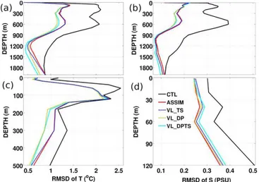
The vertical profiles of the mean RMSD of all runs against Argo and PIRATA data over the whole model domain are presented in Fig. 10. The largest temperature and salinity RMSD of the control run are attained in the top 700 m with respect to Argo data and in the top 200 m with respect to PI-RATA data. This is associated with difficulties that models have with representing the thermocline and pycnocline re-gions of sharp vertical gradients (Oke and Schiller, 2007; Xie and Zhu, 2010). When Argo data are assimilated, the vertical
Figure 9.Depth-averaged RMSD of temperature (◦C) and salinity (psu) to 2000 m against 47 999 Argo profilers in the model domain (100◦W–20◦E, 78◦S–50◦N) from 1 January 2010 to 31 Decem-ber 2012 according to the control run (black) and the prior state of the experiment ASSIM (red) and VL_DPTS (light blue).
thermohaline structure is very much improved. With respect to Argo data, the experiment ASSIM decreases the RMSD of the control run in the top 600 m from 2 to 1.3◦C and from almost 0.4 to 0.19 psu. Regarding PIRATA data, the experi-ment ASSIM reduces the RMSD values of the control run by up to 1◦C and 0.13 psu in the first 120 m. Gains with the ver-tical localization of1pare seen from 200 to 800 m and from 1200 to 2000 m. In these ranges, the experiment VL_DPTS is able to further decrease the RMSD by 0.15◦C and 0.025 psu with respect to the other assimilation runs. The vertical lo-calization of onlyT andS had almost no positive impacts on the RMSD, and contributed to slightly degradingSnear the surface when the runs were compared to PIRATA data. This is mainly because the most important HYCOM variable to determine the thermohaline structure is the model layer thickness (Thacker and Esenkov, 2002; Thacker et al., 2004; Xie and Zhu, 2010). For instance, according to HYCOM for-mulation, if the analysis increments ofT andSdecrease the density of a specific layer in comparison to its target density, the model attempts to move the lower interface downward, so that the flux of denser water across this interface increases the layer density (Bleck, 2002). The opposite happens if there is an increase of the layer density compared to its target den-sity. Therefore, the analysis increments ofT andSwill try to indirectly change the model layer thicknesses in order to ad-just the layer densities to their target densities. However, in the EnOI scheme proposed here, the assimilation of1pobs is realized before the assimilation ofT andS, and is very effective in changing the model layer thicknesses. This may explain why the model thermohaline structure is much more sensitive to the vertical localization of1prather than to the vertical localization ofT andS. The latter was studied by XZ and they also did not find any significant impact in their assimilation experiments.
Figure 10.Vertical distribution of the RMSD of temperature (◦C) and salinity (psu) against 47 999 Argo profilers and 16 PIRATA fixed moorings in the model domain (100◦W–20◦E, 78◦S–50◦N) from 1 January 2010 to 31 December 2012 according to the con-trol run (black) and the prior state of the experiment ASSIM (red), VL_TS (dark dashed blue), VL_DP (dark dashed yellow) and VL_DPTS (light blue). (a)and (b) correspond to the RMSD of
T andSwith respect to Argo observations while(c)and(d) cor-respond to the RMSD of T andS with respect to PIRATA data, respectively.
especially when correlations of the ensemble members come from a free model run that contains large discrepancies in certain regions in comparison with climatology and observa-tions. Since the co-variance matrix of the model errors in the EnOI scheme is calculated by many snapshots of the model state, the performance of the assimilation is quite dependent on the accuracy of the error co-variances (Oke et al., 2005; Xie and Zhu, 2010). Due to the biases of the ensemble mem-bers used in this work, many vertical correlations might not be well represented, especially between distant layers. Thus, since the vertical localization of layer thickness mostly keeps the correlations between adjacent layers, this strategy avoids the generation of many grid points with negative1pduring the assimilation process and makes this approach a safer way to produce a more physically consistent and reliable analysis. To investigate the spatial distribution of the RMSD ofT
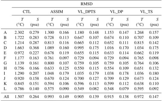
andSwith respect to Argo data above 2000 m, Table 1 con-tains the deviations for all the 12 sub-regions previously de-fined in Fig. 4. In the control run, the largest RMSDs ofTand
Sare attained in the sub-regions a, b and d with values greater than 1.6◦C and 0.27 psu. All those sub-regions are found in
the North Atlantic, where the model has the largest differ-ences in comparison with the WOA13 climatology and with Argo observations. This is particularly clear for sub-region a corresponding to the Gulf Stream region with RMSD of 2.3◦C, and for sub-region d in the Gulf of Mexico with RMSD of 0.368 psu. It should be reinforced that this grid configuration was prepared to provide boundary conditions
for higher-resolution grids focusing on the Metarea V. Hence, the control run is better adjusted with smaller RMSDs in the South Atlantic than in the North Atlantic as shown in Table 1. The maximum RMSD in the South Atlantic is attained in the sub-region i corresponding to the Brazil–Malvinas Conflu-ence with values of 1.29◦C and 0.207 psu. For all the sub-regions, the different EnOI runs are able to reduce the RMSD values ofT andS in comparison with the control run. The greatest impact of data assimilation is in the North Atlantic, where approximately 60 % of the assimilated Argo profiles are found and where the control run has its largest RMSDs. For example, the experiment ASSIM decreases the RMSD of the control run about 1◦C in the sub-regions a and b, and more than 0.17 psu for the sub-regions b, c and d. In the Gulf of Mexico, this reduction is up to 0.2 psu. On other hand, the RMSD reductions by the ASSIM run in the South Atlantic are only about 0.2◦C and 0.04 psu. Even with the large
im-pact of the Argo data assimilation, some regions still remain with large RMSDs. This is the case with the Gulf Stream, the Gulf of Mexico and the Brazil–Malvinas Confluence in the sub-regions a, d and i, respectively, where the experiments still have RMSDs greater than 1◦C and 0.145 psu. These are regions of strong gradients, variability and mesoscale eddy activity. The Gulf Stream is highly influenced by mesoscale circulation and the growth of baroclinic instability after its separation from the North American coast (Robinson et al., 1989; Spall and Robinson, 1990; Lee and Mellor, 2003). Also, the Brazil–Malvinas Confluence is characterized by a weak and warm southward Brazil Current meeting a strong, cold and less saline northward Malvinas Current, which re-sults in large contrasts in stratification and strong eddy ac-tivity (Gordon, 1989; Garzoli and Garrafo, 1989; Goni et al., 1996). Thus, the large RMSD still found in the assimilation runs in these regions can be due to lack of data, inaccuracies in the ensemble members, and limitation of the model reso-lution to solve the mesoscale circulation patterns. Similarly, XZ found that the assimilation of Argo profiles did not cap-ture the mesoscale activities in the Pacific Ocean due to the coarse model resolution, and the Kuroshio System remained with large RMSDs in their assimilation run.
In Table 1, the assimilation experiments with the best per-formances are the ones with vertical localization of layer thickness. This is particularly clear in the sub-regions a, b and c, where the experiments VL_DPTS and VL_DP are able to reduce the RMSD values up to 0.12◦C and 0.018 psu with
Table 1. RMSD of temperature (◦C) and salinity (psu) to 2000 m with respect to Argo data for the prior state of each experiment from 1 January 2010 to 31 December 2012. The calculations were performed for the whole model domain (100◦W–20◦E, 78◦S–50◦N) and for each one of the 12 sub-regions previously defined in Fig. 4.
RMSD
CTL ASSIM VL_DPTS VL_DP VL_TS
T S T S T S T S T S
(◦C) (psu) (◦C) (psu) (◦C) (psu) (◦C) (psu) (◦C) (psu)
A 2.302 0.279 1.300 0.166 1.180 0.148 1.153 0.147 1.268 0.157 B 1.722 0.283 0.728 0.113 0.647 0.107 0.674 0.110 0.707 0.109 C 1.214 0.287 0.813 0.116 0.665 0.112 0.652 0.111 0.815 0.142 D 1.663 0.368 1.089 0.160 0.995 0.175 1.016 0.170 1.034 0.175 E 0.972 0.227 0.678 0.119 0.655 0.115 0.633 0.114 0.662 0.119 F 1.177 0.163 0.761 0.097 0.729 0.094 0.729 0.094 0.765 0.098 G 1.139 0.161 0.800 0.107 0.759 0.105 0.759 0.105 0.764 0.106 H 0.756 0.166 0.633 0.125 0.550 0.115 0.554 0.109 0.651 0.132 I 1.290 0.207 1.048 0.179 1.035 0.179 1.038 0.178 1.036 0.180 J 0.920 0.158 0.670 0.124 0.700 0.127 0.709 0.129 0.673 0.124 K 0.845 0.151 0.594 0.106 0.596 0.113 0.599 0.112 0.638 0.110 L 0.786 0.140 0.575 0.090 0.549 0.082 0.548 0.079 0.595 0.092
All 1.507 0.264 0.993 0.149 0.905 0.139 0.915 0.138 0.972 0.147
the experiments VL_DP and VL_DPTS are just a little bit worse than the experiment ASSIM is the Gulf of Mexico, sub-region d, for salinity, and the sub-regions j and k in the mid-latitudes close to the AAIW formation. In general, the pairs of experiments ASSIM and VL_TS, and VL_DP and VL_DPTS, produced similar results in all sub-regions, and the strategies with vertical localization of layer thickness at-tained smaller RMSDs ofT andS. It corroborates the con-clusion that the vertical localization of1pwas more impor-tant than the vertical localization ofT andSfor the present experiments.
5.3 Adjustment of the altimetry and velocity fields As shown above, the EnOI scheme used in this work adjusts the baroclinic velocity fields via their co-variance with layer thickness in the analysis increments. This is a physically con-sistent adjustment, since the horizontal velocity fields are dominated by the slope of the isopycnal layers, which in turn generates the pressure gradient force. XZ showed that around the assimilated Argo profiles in the mid-latitudes, cyclonic and anti-cyclonic circulations develop, consistent with the large local modifications of the model layer thick-nesses and geostrophy. This is due to the nature of the co-variances, which come from an ensemble of model states and allow for the description of the anisotropic patterns of the circulation (Oke et al., 2005, 2008; Xie and Zhu, 2010). Figure 11 shows the analysis increment of layer thickness and the circulation originating in the 12th layer around an Argo profile located in the mid-latitudes of the North At-lantic on 1 January 2010 regarding the experiments ASSIM
Figure 12.30-day running SSH mean (m) of the control run (black) and the prior state of the experiment ASSIM (red), VL_TS (dark blue), VL_DP (dark yellow) and VL_DPTS (light blue) from 1 Jan-uary 2010 to 31 December 2012. The markers represent the 30-day running mean values of SSH, while the bars correspond to the stan-dard deviations of each run.
and VL_DP. The experiment ASSIM robustly induces thin-ning of layer thickness up to 200 m, and then a stronger and more anisotropic cyclonic pattern is imposed with velocity increments reaching 0.5 m s−1. Both experiments develop a cyclonic circulation around this mid-latitude Argo profile. This is coherent with the negative analysis increment of layer thickness and the negative SSH increment also shown in Fig. 11. Thus, the geostrophic balance was preserved in both experiments. Since the experiment VL_DP has limited in-fluence between distant layers, the analysis increments are smoothed and smaller velocity increments of about 0.1 m s−1 are produced. The cyclonic gyre is better represented in the VL_DP and VL_DPTS (not shown) runs, which show a more negative and more continuous increment of SSH than the AS-SIM run. The analysis constructed by this increment may be more suitable to initialize a model than the analysis by the ASSIM strategy considering the present background state and ensemble members. However, further adjustment of the velocity fields is made by the model itself during further inte-gration to balance the analysis increments after assimilation of1p,T andS.
The trend of SSH reduction by Argo data assimilation in the present experiments is confirmed in Fig. 12. It shows the 30-day SSH running mean of all experiments considering the model domain between 50◦S and 50◦N. From the beginning of the integration to December 2012, SSH is reduced from 0.22 to 0.12 m in the experiments ASSIM and VL_TS, which is compatible with the largest impact found in the first year of assimilation in Fig. 9. The VL_DP and VL_DPTS runs produce a larger reduction from 0.22 to 0.08 m. From this period on, the SSH of all assimilation experiments stabilize around these values and different SSH means are achieved in the experiments with and without vertical localization of layer thickness, but with variability very close to the control run. The diagnostic model SSH varies due to the barotropic pressure mode and especially due to the deviations in
tem-perature and salinity caused by changes in the structure of the layer thicknesses (Chin et al., 2002). Hence, this lower SSH mean in the assimilation experiments reflects the new ther-mohaline state and stratification achieved when Argo data are assimilated. The thermal expansion of seawater consti-tutes a very important component of SSH and then the re-duction of the temperature and the heat content in the assim-ilation experiments contribute strongly to the SSH decrease. For example, the heat content is positively correlated with SSH (Chambers et al., 1998; Willis et al., 2004; Dong et al., 2007). In this work, mean correlation values of 0.802, 0.815 and 0.812 between the HC and SSH are found for the ex-periments CTL, ASSIM and VL_DPTS, respectively. When comparing the monthly means of all the experiments with the WOA13 monthly means over the entire domain (not shown), the experiments VL_DP and VL_DPTS are able to decrease the HC by more than 7 MJ m−2towards the climatology. This could explain why there is a larger decrease of the mean SSH in the experiments with vertical localization of layer thick-ness.
In order to evaluate how the local changes in layer thick-ness, SSH and velocity fields affect the large-scale circula-tion, the zonal velocity along 25◦W in the upper 300 m for all the experiments and HYCOM+NCODA analysis is shown in Fig. 13. Some observed features are clearly represented in the HYCOM+NCODA analysis, such as the South At-lantic Current (SAC) south of 40◦S, the branches of the west-ward South Equatorial Current (SEC), the eastwest-ward equato-rial undercurrent (EUC) and the North Equatoequato-rial Counter-current (NECC). Modifications with respect to the control run were imposed by assimilation. However, some can be considered improvements towards the HYCOM+NCODA analysis, and some cannot. For example, there is a strong zonal current in the control run up to 0.6 m s−1between 30 and 40◦N associated with the Gulf Stream recirculation path, which is much more intense than in the HYCOM+NCODA analysis. This zonal current is reduced to 0.1–0.2 m s−1in the experiments VL_TS and VL_DPTS. However, it is displaced further south in comparison with HYCOM+NCODA anal-ysis, especially in the VL_TS run. In the experiment AS-SIM, this recirculation path is even weaker and merges in the broader eastward flow. Also, in all assimilation experiments the EUC velocity decreases from 0.6 to 0.4 m s−1and gets closer to the magnitude of the HYCOM+NCODA analysis, but the shape of its core remains the same as in the control run and is not as elongated as in the HYCOM+NCODA analy-sis. On the other hand, all data assimilation runs constrain the SAC near to the surface, while it reaches more than 300 m in the HYCOM+NCODA analysis. Finally, assimilation is not able to reduce the magnitude of the SEC and to increase the intensity of the NECC simulated by the control run.
Figure 13.Zonal velocity fields (m s−1) in the upper 300 m along 25◦W of the HYCOM+NCODA analysis, the CTL run and the prior state of the ASSIM, VL_TS and VL_DPTS runs from 1 Jan-uary 2010 to 31 December 2012. The black solid and black dashed lines denote the contours of 0.1 m s−1and−0.1 m s−1, respectively.
undercurrent maximum in the east and a too thick and strong westward current in the west were produced. In the present work, a few modifications were observed in the equatorial Atlantic region as well, but with smaller intensity than in the mid-latitudes. It should be noted that the geostrophic bal-ance that holds in most of the ocean interior loses importbal-ance close to the equator. Therefore, the equatorial current system should be less sensitive to analysis increments by Argo data
assimilation, so that changes in this region may be mostly attributed to remote impacts from the assimilation in extra-equatorial regions.
In the present work, the discrepancies of the model free run and its variability with respect to climatology and ob-servations are an important limitation for the assimilation to produce the correct analysis increments, particularly for the large-scale circulation. For this reason, many works point out that the model biases should be considered during the assimilation process (Reynolds et al., 1996; Dee and Silva, 1998; Bell et al., 2004; Dee, 2005; Xie and Zhu, 2010). Also, improving the co-variances of the ensemble mem-bers may lead to more accurate analyses (Oke et al., 2008; Xie and Zhu, 2010). In addition to the comparison with the HYCOM+NCODA analysis, the surface velocity fields of the assimilation runs were compared to the OSCAR fields. Again, the results did not provide a clear signal about the im-pact of Argo data assimilation on the surface currents. The RMSD of U and V with respect to OSCAR were reduced by less than 5 % in comparison to the control run.
6 Conclusions and discussion
In this work, an EnOI scheme to assimilate Argo data into HYCOM was successfully constructed and implemented. The first results were evaluated against observations and analyses over the Atlantic Ocean. The EnOI scheme was based mostly on the work of XZ. A key variable in the as-similation algorithm was the observed model layer thickness,
1pobs, constructed from the Argo temperature (T) and salin-ity (S) profiles, according to TE. First,1pobswas assimilated and the analysis state vector considered not only the model layer thickness, but also the baroclinic velocities. This pro-cedure is physically consistent, since the horizontal veloc-ity fields are dominated by the difference between the layer depths, which will be the responsible for the pressure gradi-ent force. After that, with the previously adjusted model layer thicknesses,T andS were assimilated in separate steps. Fi-nally,T was diagnosed below the mixed layer through the seawater equation of state following the best results found in XZ. Thus, this EnOI scheme respects the hybrid nature of the HYCOM vertical coordinate system and allows for the restructuring of the isopycnal layer thicknesses and veloci-ties with the assimilation of1pobs. Also, a sensitivity study was performed considering different vertical localizations of the model error co-variance matrix, involving the variables
T,Sand especially1p. Five integrations were realized from 1 January 2010 to 31 December 2012. The study of the im-pact of the vertical localization of1pis an original contribu-tion of this work.
at least 34 % (44 %) forT (S), regarding the control run over the whole domain. Spatially, the RMSD ofT andSdecreased for all the 12 selected sub-regions of the domain with remark-able corrections in the depth of the 20◦C isotherm and heat
content in the upper 300 m towards WOA13, particularly in the North Atlantic. Also, the reorganization of the isopyc-nal layers by the assimilation of1pobshas provided a large reduction of the diagnosed SSH in the model, reflecting the new thermohaline state achieved by Argo data assimilation. Indeed, the correction of layer thickness played a role in cor-recting the model thermohaline structure and stratification, as stated in previous data assimilation works with HYCOM (Thacker and Esenkov, 2002; Chin et al., 2002; Thacker et al., 2004; Xie and Zhu, 2010).
The vertical localization ofT andS did not produce any significant impact in the assimilation experiments, which is consistent with the results found in XZ. However, the exper-iments VL_DP and VL_DPTS with vertical localization of
1pwere able to decrease the RMSD ofT (S) from 0.993◦C
(0.149 psu) to 0.905◦C (0.138 psu) in the whole model do-main with respect to the other assimilation runs. This im-provement was especially seen in the North Atlantic, where the ensemble members and background had their largest bi-ases with respect to observations and climatology. The exper-iments with vertical localization of1pdecreased by 66 % the number of grid points with negative1pgenerated during the assimilation process by constraining the vertical co-variances between more distant layers, and then reducing the degrees of freedom offered by the ensemble members. This result re-inforces how important the quality of the ensemble members is in order to improve the performance of the assimilation, particularly in the EnOI scheme, in which the ensemble is stationary in time and does not evolve with the model in-tegration as in the EnKF (Evensen, 2003; Oke et al., 2005, 2008). In future works with EnOI, the quality of the ensem-ble members should be taken into account. For example, long reanalysis with Argo data assimilation should be performed first to provide new and better ensemble members and, there-fore, improve the accuracy of the model error co-variance to be employed in a new assimilation run. If more accurate en-semble members are employed, it is expected that the strong vertical localization of1pwill not lead to improvements in the analysis.
Despite the evidence that the assimilation experiments caused a strong SSH reduction in the model domain and that the analysis increments of 1p and velocities were locally consistent, there was not a clear improvement in the large-scale circulation. The assimilation schemes were simply bias blind here. The model biases should be considered in future studies to better analyze the impact of Argo data assimi-lation in the large-scale circuassimi-lation. According to Oke and Schiller (2007), the role of Argo data assimilation is mainly to constrain the thermohaline structure of the model, espe-cially for salinity, and this was obtained in the present work. To constrain the SST andT in the mixed layer, the
assimi-lation of SST should be performed, and to correct the upper mesoscale circulation, the assimilation of SLA is needed.
The present work was a key step forward in two major directions. First, it was the basis for the future implemen-tation of assimilation in the other REMO higher-resolution grids. For the current domain with 760×480 horizontal grid points, the Argo data assimilation code took around 12 min of CPU on 32 2 GHz processors to assimilate approximately 150 ArgoT–S profiles. Therefore, it can be easily used in operational mode. Second, it served as the backbone to con-struct the assimilation code for along-track satellite altimetry data and SST analyses that will form the REMO Ocean Data Assimilation System into HYCOM (RODAS_H) for opera-tional and research purposes (Tanajura et al., 2014).
Acknowledgements. This work was financially supported by PETROBRAS and Agência Nacional de Petróleo, Gás Natural e Biocombustíveis (ANP), Brazil, via the Oceanographic Modeling and Observation Network (REMO). The authors of this manuscript would like to acknowledge the support of the National Research Council (CNPq), Ministry of Science, Technology and Innovation of Brazil (proc. 130032/2012-3), and the support of the CAPES Foundation, Ministry of Education of Brazil (proc. BEX 3957/13-6).
Edited by: N. Wells
References
Bell, M. J., Martin, M. J., and Nichols, N. K.: Assimilation of data into an ocean model with systematic errors near the equator, Q. J. Roy. Meteor. Soc., 130, 873–893, 2004.
Belyaev, K. P., Tanajura, C. A. S., and Tuchkova, N. P.: Comparison of Methods for Argo Drifters Data Assimilation into a Hydrody-namical Model of the Ocean, Oceanology, 52, 593–603, 2012. Bleck, R.: An oceanic general circulation model framed in hybrid
isopycnic-Cartesian coordinates, Ocean Modell., 4, 55–88, 2002. Bleck, R. and Smith, L. T.: A wind-driven isopycnic coordinate model of the north and equatorial atlantic ocean. 1. Model devel-opment and supporting experiments, J. Geophys. Res., 95, 3273– 3285, 1990.
Boyer, T. and Mishonov, A.: World Ocean Atlas 2013 Product Doc-umentation, Technical Ed. NOAA Atlas NEDSIS, 14 pp., 2013. Brydon, D., Sun, S., and Bleck, R.: A new approximation of the
equation of state for sea water, suitable for numerical ocean mod-els, J. Geophys. Res., 104, 1537–1540, 1999.
Carton, J. A. and Giese, B. S.: A Reanalysis of Ocean Climate Using Simple Ocean Data Assimilation (SODA), Mon. Weather Rev., 136, 2999–3017, 2008.
Chambers, D., Tapley, B., and Stewart, R.: Measuring heat stor-age changes in the equatorial Pacific: A comparison between TOPEX altimetry and tropical atmosphere-ocean buoys, J. Geo-phys. Res., 103, 591–597, 1998.