www.geosci-model-dev.net/9/431/2016/ doi:10.5194/gmd-9-431-2016
© Author(s) 2016. CC Attribution 3.0 License.
FPLUME-1.0: An integral volcanic plume model accounting for ash
aggregation
A. Folch1, A. Costa2, and G. Macedonio3
1CASE Department, Barcelona Supercomputing Center, Barcelona, Spain
2Istituto Nazionale di Geofisica e Vulcanologia, Sezione di Bologna, Bologna, Italy 3Istituto Nazionale di Geofisica e Vulcanologia, Sezione di Napoli, Naples, Italy Correspondence to:A. Folch ([email protected])
Received: 22 July 2015 – Published in Geosci. Model Dev. Discuss.: 17 September 2015 Revised: 22 December 2015 – Accepted: 5 January 2016 – Published: 2 February 2016
Abstract. Eruption source parameters (ESP) characterizing volcanic eruption plumes are crucial inputs for atmospheric tephra dispersal models, used for hazard assessment and risk mitigation. We present FPLUME-1.0, a steady-state 1-D (one-dimensional) cross-section-averaged eruption column model based on the buoyant plume theory (BPT). The model accounts for plume bending by wind, entrainment of ambient moisture, effects of water phase changes, particle fallout and re-entrainment, a new parameterization for the air entrain-ment coefficients and a model for wet aggregation of ash par-ticles in the presence of liquid water or ice. In the occurrence of wet aggregation, the model predicts aneffectivegrain size distribution depleted in fines with respect to that erupted at the vent. Given a wind profile, the model can be used to deter-mine the column height from the eruption mass flow rate or vice versa. The ultimate goal is to improve ash cloud disper-sal forecasts by better constraining the ESP (column height, eruption rate and vertical distribution of mass) and the effec-tive particle grain size distribution resulting from eventual wet aggregation within the plume. As test cases we apply the model to the eruptive phase-B of the 4 April 1982 El Chichón volcano eruption (México) and the 6 May 2010 Eyjafjalla-jökull eruption phase (Iceland). The modular structure of the code facilitates the implementation in the future code ver-sions of more quantitative ash aggregation parameterization as further observations and experiment data will be available for better constraining ash aggregation processes.
1 Introduction
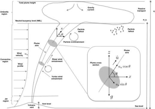
Volcanic plumes (e.g. Sparks, 1997) are turbulent multi-phase flows containing volcanic gas, entrained ambient air and moisture and tephra, consisting on both juvenile (result-ing from magma fragmentation), crystal and lithic (result(result-ing from wall rock erosion) particles ranging from metre-sized blocks to micron-sized fine ash (diameter ≤63 µm). Sus-tained volcanic plumes present a negatively buoyant basal thrust region where the mixture rises due to its momentum. As ambient air is entrained by turbulent mixing, it heats and expands, thereby reducing the average density of the mixture. It leads to a transition to the convective region, in which pos-itive buoyancy drives the mixture up to the so-called neutral buoyancy level (NBL), where the mixture density equals that of the surrounding atmosphere. Excess of momentum above the NBL (overshooting) can drive the mixture higher forming the umbrella region, where tephra disperses horizontally first as a gravity current (e.g. Costa et al., 2013; Carazzo et al., 2014) and then under passive wind advection forming a vol-canic cloud (see Fig. 1).
param-θ s
Volcano vent Wind profile
Jet region Convective
region Umbrella
region
Vortex wind entrainment Shear wind entrainment
Plume axis Neutral buoyancy level (NBL)
uacosθ
θ
uasinθ
Plume cross section
ˆ
u Total plume height
Particle fallout
Particle re-entrainment
z
g
x
Wind velocity ua
Gravity current
Particle fallout
Passive transport
H_b H_t
Sealevel Plume
axis
Ventlevel
Figure 1.Sketch of an axisymmetric volcanic plume raising in a wind profile. Three different regions (jet thrust, convective thrust and
umbrella) are indicated, with the convective region reaching a heightHb(that of the neutral buoyancy level), and the umbrella region raising up toHtabove the sea level (a.s.l.). The inset plot details a plume cross section perpendicular to the plume axis, inclined of an angleθwith
respect to the horizontal.
eters but, given their high computational cost, coupling with atmospheric dispersal models at an operational level is still unpractical. Moreover, even sophisticated 3-D multiphase models can have serious problems to accurately describe the physical processes related to closure equations, compu-tational spatial resolution, etc. For this reason, simpler 1-D cross-section-averaged models or even empirical relation-ships between plume height and eruption rate (e.g. Mastin et al., 2009; Degruyter and Bonadonna, 2012) are used in practice to furnish eruption source parameters (ESP) to at-mospheric transport models, the results of which strongly de-pend on the source term quantification (i.e. determination of plume height, eruption rate, vertical distribution of mass and particle grain size distribution).
Many plume models based on the BPT have been pro-posed after the seminal studies of Wilson (1976) and Sparks (1986) to address different aspects of plume dynamics. For example, Woods (1993) proposed a model to include the la-tent heat associated with condensation of water vapour and quantify its effects upon the eruption column. Ernst et al. (1996) presented a model considering particle sedimentation and re-entrainment from plume margins. Bursik (2001) anal-ysed how the interaction with wind enhances entrainment of air, plume bending and decrease of the total plume height for a given eruption rate. Several other plume models ex-ist (see Costa et al., 2015, and references therein), consider-ing different modellconsider-ing approaches, simplifyconsider-ing assumptions and model parameterizations. It is well recognized that the
values of the air entrainment coefficients have a large influ-ence on the results of the plume models. On the other hand, volcanic ash aggregation (e.g. Brown et al., 2012) can occur within the eruption column or, under certain circumstances, downstream within the ash cloud (Durant et al., 2009). In any case, the formation of ash aggregates (with typical sizes around few hundreds of µm and less dense than the primary particles) dramatically impacts particle transport dynamics thereby reducing the atmospheric residence time of aggre-gating particles and promoting the premature fallout of fine ash. As a result, atmospheric transport models neglecting ag-gregation tend to overestimate far-range ash cloud concen-trations, leading to an overestimation of the risk posed by ash clouds on civil aviation and an underestimation of ash loading in the near field. So far, no plume model tries to pre-dict the formation of ash aggregates in the eruptive column and how it affects the particle grain size distribution erupted at the vent. This can be explained in part because aggrega-tion mechanisms are complex and not fully understood yet, although theoretical models have been proposed for wet ag-gregation (Costa et al., 2010; Folch et al., 2010).
dy-namics, particle properties, and amount of liquid water and ice existing in the plume. The modelling of aggregation in the plume, proposed here for the first time, allows our model to predict an effective total grain size distribution (TGSD) depleted in fines with respect to that erupted at the vent. The ultimate goal is to improve ash cloud forecasts by better con-straining these relevant aspects of the source term. In this manuscript, we present first the governing equations for the plume and aggregation models and then apply the combined model to two test cases, the eruptive phase-B of the 1982 El Chichón volcano eruption (México) and the 6 May 2010 Ey-jafjallajökull eruption phase (Iceland).
2 Physical plume model
We consider a volcanic plume as a multiphase mixture of volatiles, suspended particles (tephra) and entrained ambient air. For simplicity, water (in vapour, liquid or ice phase) is assumed the only volatile species, being either of magmatic origin or incorporated through the ingestion of moist ambient air. Erupted tephra particles can form by magma fragmen-tation or by erosion of the volcanic conduit, and can vary notably in size, shape and density. For historical reasons, field volcanologists describe the continuous spectrum of par-ticle sizes in terms of the dimensionless8-scale (Krumbein, 1934):
d(8)=d∗2−8=d∗e−8log 2, (1) where d is the particle size and d∗=10−3m is a refer-ence length (i.e. 2−8is the direction-averaged particle size expressed in mm). The vast majority of modelling strate-gies, discretize the continuous particle grain size distribution (GSD) by grouping particles inndifferent8-bins, each with an associated particle mass fraction (the models based on moments (e.g. de’ Michieli Vitturi et al., 2015) are the ex-ception). Because particle size exerts a primary control on sedimentation, 8-classes are often identified with terminal settling velocity classes although, strictly, a particle settling velocity class is defined not only by particle size but also by its density and shape. We propose a model for volcanic plumes as a multiphase homogeneous mixture of water (in any phase), entrained air, and n particle classes, including a parameterization for the air entrainment coefficients and a wet aggregation model. Because the governing equations based upon the BPT are not adequate above NBL, we also propose a new semi-empirical model to describe such a re-gion.
2.1 Governing equations
The steady-state cross-section-averaged governing equations for axisymmetric plume motion in a turbulent wind (see
Fig. 1) are the following (for the meaning of the used sym-bols see Tables 1 and 2):
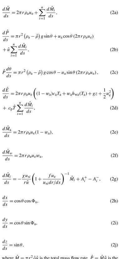
dMˆ
ds =2π rρaue+
n X
i=1 dMˆi
ds , (2a)
dPˆ ds =π r
2 ρa
− ˆρgsinθ+uacosθ (2π rρaue)
+ ˆu
n X
i=1 dMˆi
ds , (2b)
ˆ
Pdθ ds =π r
2 ρ a− ˆρ
gcosθ−uasinθ (2π rρaue) , (2c)
dEˆ
ds =2π rρaue
(1−wa)caTa+wahwa(Ta)+gz+1 2u
2 e
+ cpTˆ
n X
i=1 dMˆi
ds , (2d)
dMˆa
ds =2π rρaue(1−wa), (2e)
dMˆw
ds =2π rρauewa, (2f)
dMˆi
ds = − χ usi
ruˆ
1+ f ue
usidr/ds −1
ˆ
Mi+A+i −A−i , (2g)
dx
ds =cosθcos8a, (2h)
dy
ds =cosθsin8a, (2i)
dz
ds =sinθ, (2j)
whereMˆ =π r2ρˆuˆis the total mass flow rate,Pˆ= ˆMuˆis the total axial (stream-wise) momentum flow rate,θis the plume bent over angle with respect to the horizontal (i.e.θ=90◦for a plume raising vertically),Eˆ = ˆM(Hˆ+gz+12uˆ2)is the total energy flow rate,Hˆ is the enthalpy flow rate of the mixture,
ˆ
T= ˆT (H )ˆ is the mixture temperature, Mˆa is the mass flow rate of dry air,Mˆw= ˆMxˆw is the mass flow rate of volatiles
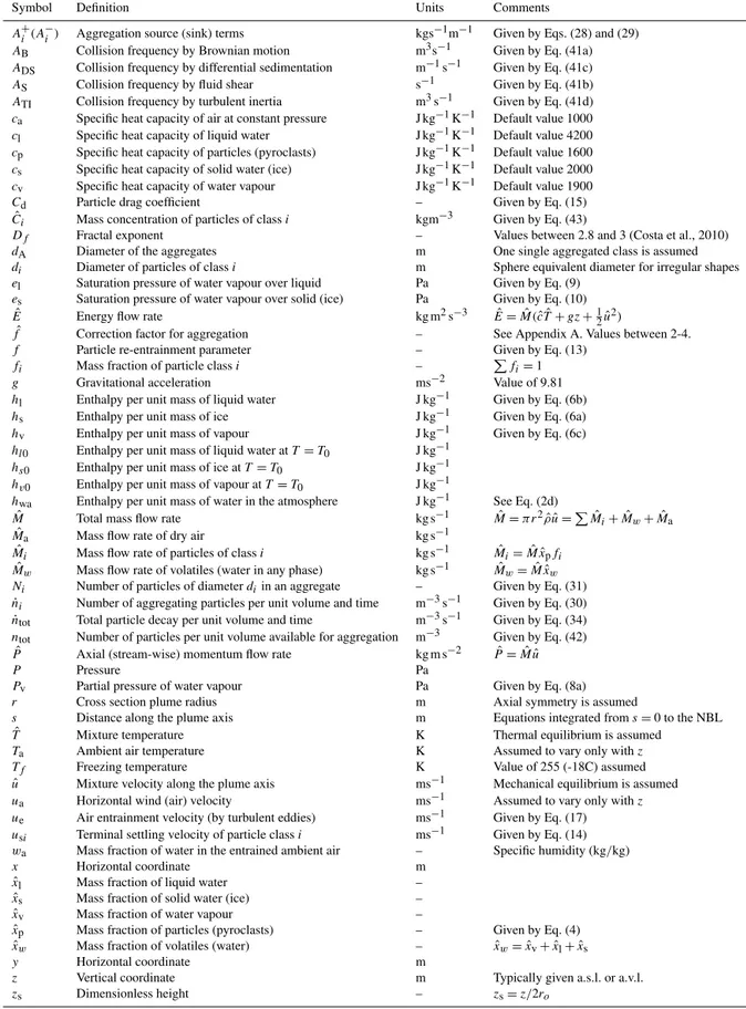
Table 1.List of Latin symbols. Quantities with a hat denote bulk (top-hat averaged) quantities. Throughout the text, the subindex o (e.g.Mˆo, ˆ
uo) indicates values of quantities at the vent (s=0).
Symbol Definition Units Comments
A+i(A−i) Aggregation source (sink) terms kgs−1m−1 Given by Eqs. (28) and (29)
AB Collision frequency by Brownian motion m3s−1 Given by Eq. (41a) ADS Collision frequency by differential sedimentation m−1s−1 Given by Eq. (41c) AS Collision frequency by fluid shear s−1 Given by Eq. (41b) ATI Collision frequency by turbulent inertia m3s−1 Given by Eq. (41d) ca Specific heat capacity of air at constant pressure J kg−1K−1 Default value 1000 cl Specific heat capacity of liquid water J kg−1K−1 Default value 4200 cp Specific heat capacity of particles (pyroclasts) J kg−1K−1 Default value 1600 cs Specific heat capacity of solid water (ice) J kg−1K−1 Default value 2000 cv Specific heat capacity of water vapour J kg−1K−1 Default value 1900 Cd Particle drag coefficient – Given by Eq. (15)
ˆ
Ci Mass concentration of particles of classi kgm−3 Given by Eq. (43)
Df Fractal exponent – Values between 2.8 and 3 (Costa et al., 2010)
dA Diameter of the aggregates m One single aggregated class is assumed
di Diameter of particles of classi m Sphere equivalent diameter for irregular shapes
el Saturation pressure of water vapour over liquid Pa Given by Eq. (9)
es Saturation pressure of water vapour over solid (ice) Pa Given by Eq. (10)
ˆ
E Energy flow rate kg m2s−3 Eˆ= ˆM(cˆTˆ+gz+1 2uˆ2)
ˆ
f Correction factor for aggregation – See Appendix A. Values between 2-4.
f Particle re-entrainment parameter – Given by Eq. (13)
fi Mass fraction of particle classi – Pfi=1 g Gravitational acceleration ms−2 Value of 9.81
hl Enthalpy per unit mass of liquid water J kg−1 Given by Eq. (6b) hs Enthalpy per unit mass of ice J kg−1 Given by Eq. (6a)
hv Enthalpy per unit mass of vapour J kg−1 Given by Eq. (6c) hl0 Enthalpy per unit mass of liquid water atT=T0 J kg−1
hs0 Enthalpy per unit mass of ice atT=T0 J kg−1
hv0 Enthalpy per unit mass of vapour atT=T0 J kg−1
hwa Enthalpy per unit mass of water in the atmosphere J kg−1 See Eq. (2d)
ˆ
M Total mass flow rate kg s−1 Mˆ=π r2ρˆuˆ=P ˆ
Mi+ ˆMw+ ˆMa
ˆ
Ma Mass flow rate of dry air kg s−1
ˆ
Mi Mass flow rate of particles of classi kg s−1 Mˆ i= ˆMxˆpfi
ˆ
Mw Mass flow rate of volatiles (water in any phase) kg s−1 Mˆw= ˆMxˆw Ni Number of particles of diameterdiin an aggregate – Given by Eq. (31)
˙
ni Number of aggregating particles per unit volume and time m−3s−1 Given by Eq. (30)
˙
ntot Total particle decay per unit volume and time m−3s−1 Given by Eq. (34) ntot Number of particles per unit volume available for aggregation m−3 Given by Eq. (42)
ˆ
P Axial (stream-wise) momentum flow rate kg m s−2 Pˆ= ˆMuˆ
P Pressure Pa
Pv Partial pressure of water vapour Pa Given by Eq. (8a) r Cross section plume radius m Axial symmetry is assumed
s Distance along the plume axis m Equations integrated froms=0 to the NBL ˆ
T Mixture temperature K Thermal equilibrium is assumed
Ta Ambient air temperature K Assumed to vary only withz Tf Freezing temperature K Value of 255 (-18C) assumed ˆ
u Mixture velocity along the plume axis ms−1 Mechanical equilibrium is assumed
ua Horizontal wind (air) velocity ms−1 Assumed to vary only withz ue Air entrainment velocity (by turbulent eddies) ms−1 Given by Eq. (17) usi Terminal settling velocity of particle classi ms−1 Given by Eq. (14) wa Mass fraction of water in the entrained ambient air – Specific humidity (kg/kg)
x Horizontal coordinate m
ˆ
xl Mass fraction of liquid water –
ˆ
xs Mass fraction of solid water (ice) –
ˆ
xv Mass fraction of water vapour –
ˆ
xp Mass fraction of particles (pyroclasts) – Given by Eq. (4)
ˆ
xw Mass fraction of volatiles (water) – xˆw= ˆxv+ ˆxl+ ˆxs
y Horizontal coordinate m
z Vertical coordinate m Typically given a.s.l. or a.v.l.
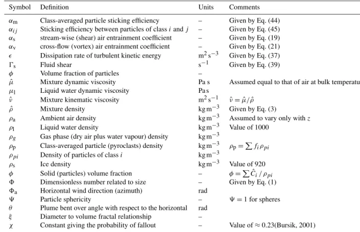
Table 2.List of greek symbols. Quantities with a hat denote bulk (top-hat averaged) quantities.
Symbol Definition Units Comments
αm Class-averaged particle sticking efficiency – Given by Eq. (44)
αij Sticking efficiency between particles of classiandj – Given by Eq. (45)
αs stream-wise (shear) air entrainment coefficient – Given by Eq. (19)
αv cross-flow (vortex) air entrainment coefficient – Given by Eq. (21)
ǫ Dissipation rate of turbulent kinetic energy m2s−3 Given by Eq. (37)
Ŵs Fluid shear s−1 Given by Eq. (39)
φ Volume fraction of particles –
ˆ
µ Mixture dynamic viscosity Pa s Assumed equal to that of air at bulk temperature
µl Liquid water dynamic viscosity Pa s
ˆ
ν Mixture kinematic viscosity m2s−1 νˆ= ˆµ/ρˆ ˆ
ρ Mixture density kg m−3 Given by Eq. (3)
ρa Ambient air density kg m−3 Assumed to vary only withz
ρl Liquid water density kg m−3 Value of 1000
ρg Gas phase (dry air plus water vapour) density kg m−3
ρp Class-averaged particle (pyroclasts) density kg m−3 ρp=Pfiρpi
ρpi Density of particles of classi kg m−3
ρs Ice density kg m−3 Value of 920
φ Solid (particles) volume fraction – φ=Pˆ
Ci/ ρpi
8 Dimensionless number related to size – Given by Eq. (1)
8a Horizontal wind direction (azimuth) rad
9 Particle sphericity – 9=1 for spheres
θ Plume bent over angle with respect to the horizontal rad
ξ Diameter to volume fractal relationship –
χ Constant giving the probability of fallout – Value of≈0.23(Bursik, 2001)
per unit mass of the water in the atmosphere,Mˆi= ˆMxˆpfiis
the mass flow rate of particles of classi(i=1:n),x andy are the horizontal coordinates,zis height andsis the distance along the plume axis (see Tables 1 and 2 for the definition of all symbols and variables appearing in the manuscript).
The equations above derive from conservation princi-ples assuming axial (stream-wise) symmetry and consider-ing bulk quantities integrated over a plume cross section us-ing a top-hat profile in which a generic quantity φ has a constant valueφ (s)ˆ at a given plume cross section and van-ishes outside (here we refer to section-averaged quantities as bulk quantities, denoted by a hat). We have derived these equations by combining formulations from different previ-ous plume models (Netterville, 1990; Woods, 1993; Ernst et al., 1996; Bursik, 2001; Costa et al., 2006; Woodhouse et al., 2013) in order to include in a single model effects from plume bending by wind, particle fallout and re-entrainment at plume margins, transport of volatiles (water) accounting also for ingestion of ambient moisture, phase changes (water vapour condensation and deposition) and particle aggrega-tion. Equation (2j) expresses the conservation of total mass, accounting in the right-hand side (rhs) for the mass of air entrained through the plume margins and the loss/gain of mass by particle fallout/re-entrainment. Equation (2b) and (2c) express the conservation of axial (stream-wise) and ra-dial momentum, respectively, accounting on the rhs for
con-tributions from buoyancy (first term), entrainment of air, and particle fallout/re-entrainment. Note that generally the buoy-ancy term, acting only along the vertical directionz, repre-sents a sink of momentum in the basal gas-thrust jet region (whereρ > ρˆ a) and a source of momentum where the plume is positively buoyant (ρ < ρˆ a). Equation (2d) expresses the conservation of energy, accounting on the rhs for gain of en-ergy (enthalpy, potential and kinetic) by ambient air entrain-ment (first term), loss/gain by particle fallout/re-entrainentrain-ment (second term), and gain of energy by conversion of water vapour into liquid (condensation) or into ice (deposition). Equation (2e), (2f) and (2g) express, respectively, the conser-vation of mass of dry air, water (vapour, liquid and ice) and solid particles. The latter set of equations, one for each parti-cle class, account on the rhs for partiparti-cle re-entrainment (first term), particle fallout (second term) and particle aggregation. Here we have included to terms (A+i andA−i ) that account for the creation of mass from smaller particles aggregating into particle classiand for the destruction of mass resulting from particles of class i contributing to the formation of larger-size aggregates. Finally, Eq. (2h) to (2j) determine the 3-D plume trajectory as a function of the length parameters. All these equations constitute a set of 9+nfirst order ordinary differential equations insfor 9+nunknowns:M,ˆ Pˆ,θ,E,ˆ
ˆ
using the definitions of M-ˆ Pˆ-E, the equations can also beˆ expressed in terms ofu-r-ˆ Tˆ given the bulk density.
Assuming an homogeneous mixture, the bulk densityρˆof the mixture is
1
ˆ
ρ =
ˆ
xp ρp+
ˆ
xl ρl+
ˆ
xs ρs +
(1− ˆxp− ˆxl− ˆxs) ρg
, (3)
wherexp,ˆ xlˆ andxsˆ are, respectively, the mass fractions of particles, liquid water and ice, ρp is the class-weighted av-erage density of particles (pyroclasts), ρl andρs are liquid water and ice densities, andρg is the gas phase (i.e. dry air
plus water vapour) density. Under the assumption of mechan-ical equilibrium (i.e. assuming the same bulk velocity uˆfor all phases and components) it holds that
ˆ
xp=
P ˆ
Mi ˆ
M =
P ˆ
Mi P ˆ
Mi+ ˆMw+ ˆMa
. (4)
The enthalpy flow rate of the mixture is a non-decreasing function of the temperatureTˆ given by
ˆ
H= ˆM[xacaTˆ+xpcpTˆ+xvhv(T )ˆ +xlhl(T )ˆ +xshs(T )ˆ ], (5) wherehv,hl andhs are, respectively, the enthalpy per unit mass of water vapour, liquid and ice:
hs(T )ˆ =csT ,ˆ (6a)
hl(T )ˆ =hl0+cl(Tˆ−T0), (6b)
hv(T )ˆ =hv0+cv(Tˆ−T0), (6c) wherecs=2108 J K−1kg−1is the specific heat of ice,T0is a reference temperature, hl0=3.337×10⁵J kg−1 is the en-thalpy of the liquid water at the reference temperature,cl= 4187 J K−1kg−1 is the specific heat of liquid water,hv0= 2.501×10⁶J kg−1is the enthalpy of vapour water at the ref-erence temperature and cv=1996 J K−1kg−1 is the specific heat of vapour water. For convenience, the reference temper-atureT0 is taken equal to the temperature of triple point of the water (T0=273.15 K). The energy and the enthalpy flow rate are related by
ˆ
E= ˆH+ ˆM(gz+1 2u
2).
(7) For the integration of Eq. (2d) and for evaluating the aggre-gation rate terms in Eq. (2g), the temperatureTˆand the mass fractions of ice (xs), liquid water (xl) and vapour (xv) need to be evaluated. These quantities are obtained by the direct inversion of Eq. (5), with the use of Eqs. (2d) and (7) and by assuming that the pressure inside the plumeP is equal to the atmospheric pressure at the same altitude (z).
The model uses a pseudo-gas assumption considering that the mixture of air and water vapour behaves as an ideal gas: P =Pv+Pa; Pv=nvP ; Pa=naP , (8a)
nv= xv/mv xv/mv+xa/ma ;
na= xa/ma xv/mv+xa/ma
, (8b)
wherePvandPaare, respectively, the partial pressures of the water vapour and of the air in the plume,nvandna are the molar fractions of vapour and air in the gas phase (nv+na= 1) andmv=0.018 kg/mole andma=0.029 kg/mole are the molar weights of vapour and air. Following Woods (1993) and Woodhouse et al. (2013), we consider that, if the air-water mixture becomes saturated in air-water vapour, conden-sation or deposition occurs and the plume remains just sat-urated. This assumption implies that the partial pressure of water vapourPvequals the saturation pressure of vapour over liquid (el) or over ice (es) at the bulk temperature, and the saturation pressures over liquid and ice are given (in hPa) by (Murphy and Koop, 2005)
el=6.112 exp 17.67Tˆ−273.16
ˆ
T−29.65
!
(9)
loges= −9.097( 273.16
ˆ
T −1)−3.566 log( 273.16
ˆ
T ),
+0.876(1− Tˆ
273.16)+log(6.1071). (10)
Equation (9) holds forTˆ ≥Tf and Eq. (10) is valid forTˆ ≤
Tf, whereTf is the temperature of the triple point of the
water (here set atPf =611.2 Pa,Tf =273.16 K). Therefore,
ifT > Tˆ f andPv< el, the plume is undersaturated and there is no water vapour condensation (i.e.xˆv= ˆxwandxˆl= ˆxs= 0). In contrast, ifPv≥el, the vapour in excess is immediately converted into liquid and
(P−el) nv=elna
ˆ
xs=0
ˆ
xl= ˆxw− ˆxv. (11)
The vapour and air mass fractionsxv andxa are evaluated by combining Eq. (11) and (8b). On the other hand, ifTˆ ≤ Tf andPv< es the plume is undersaturated and there is no water vapour deposition. In contrast, ifPv≥es, the vapour in excess is immediately converted into ice and
(P−es) nv=esna
ˆ
xl=0
ˆ
xs= ˆxw− ˆxv. (12)
For the particle re-entrainment parameterf we adopt the fit proposed by Ernst et al. (1996) using data for plumes not affected by wind:
f =0.43
1+ "
0.78usP 1/4
o
Fo1/2 #6
−1
, (13)
wherePo=ro2uˆ2oandFo=ro2uˆoHˆoare the specific
momen-tum and thermal fluxes at the vent (s=0), andHˆois the
en-thalpy per unit mass of the mixture at the vent. This expres-sion may overestimate re-entrainment for bent over plumes (Bursik, 2001). Finally, particle terminal settling velocityusi
is parameterized as (Costa et al., 2006; Folch et al., 2009)
usi= s
4g(ρpi− ˆρ)di
3Cdρˆ
, (14)
wheredi is the class particle diameter andCdis a drag coef-ficient that depends on the Reynolds numberRe=diusiρˆ/µ.ˆ
Several empirical fits exist for drag coefficients of spherical and non-spherical particles (e.g. Wilson and Huang, 1979; Arastoopour et al., 1982; Ganser, 1993; Dellino et al., 2005). In particular, Ganser (1993) gave a fit valid over a wide range of particle sizes and shapes covering the spectrum of volcanic particles considered in volcanic column models (lapilli and ash):
Cd= 24 ReK1
n
1+0.1118[Re (K1K2)]0.6567o
+ 0.4305K2
1+ReK3305 1K2
, (15)
whereK1andK2are two shape factors depending on par-ticle sphericity, 9, and particle orientation. Given that the Cd depends on Re(i.e. onus), Eq. 14 is solved iteratively using a bisection algorithm. Given a closure equation for the turbulent air entrainment velocity ue, and an aggrega-tion model (defining the mass aggregaaggrega-tion coefficients A+i andA−i ), Eq. (2j) to (2i) can be integrated along the plume axis from the inlet (volcanic vent) up to the neutral buoy-ancy level. Inflow (boundary) conditions are required at the vent (s=0) for, e.g., total mass flow rateMˆo, bent over angle
θo=90◦, temperatureTˆo, exit velocityuˆo, fraction of water ˆ
xwo, null air mass flow rateMˆa=0, vent coordinates (xo,yo
andzo), and mass flow rate for each particle classMˆio. The
latter is obtained from the total mass flow rate at inflow given the particle grain size distribution at the vent:
ˆ
Mio=fioMˆo(1− ˆxwo), (16)
wherefiois the mass fraction of classiat the vent.
2.2 Entrainment coefficients
Turbulent entrainment of ambient air plays a key role on the dynamics of jets and buoyant plumes. In the basal region of
volcanic columns, the rate of entrainment dictates whether the volcanic jet enters into a collapse regime by exhaustion of momentum before the mixture becomes positively buoyant, or whether it evolves into a convective regime reaching much higher altitudes. Early laboratory experiments (e.g. Hewett et al., 1971) already indicated that the velocity of entrainment of ambient air is proportional to velocity differences parallel and normal to the plume axis (see inset in Fig. 1):
ue=αs| ˆu−uacosθ| +αv|uasinθ|, (17) where αs and αv are dimensionless coefficients that con-trol the entrainment along the stream-wise (shear) and cross-flow (vortex) directions, respectively. Note that, in absence of wind (i.e.ua=0), the equation above reduces toue=αsuˆ and the classical expression for entrainment velocity of Mor-ton et al. (1956) is recovered. In contrast, under a wind field, both along-plume (proportional to the relative velocity differ-ences parallel to the plume) and cross-flow (proportional to the wind normal component) contributions appear. However it is worth noting that Eq. (17) has not a solid theoretical jus-tification and is used on an empirical basis. A vast literature exists regarding the experimental (e.g. Dellino et al., 2014) and numerical (e.g. Suzuki and Koyaguchi, 2009) determina-tion of entrainment coefficients for jets and buoyant plumes. Based on these results, most 1-D integral plume models available in literature consider (i) same constant entrainment coefficients along the plume, (ii) piecewise constant values at the different regions or, (iii) piecewise constant values cor-rected by a factorpρ/ρaˆ (Woods, 1993). Typical values for the entrainment coefficients derived from experiments are of the order ofαs≈0.07–0.1 for the jet region, αs≈0.1– 0.17 for the buoyant region andαv≈0.3–1.0 (e.g. Devenish, 2013). However, more recent experimental (Kaminski et al., 2005) and sensitivity analysis numerical studies (Charpen-tier and Espíndola, 2005) concluded that piecewise constant functions are valid only as a first approach, implying that 1-D integral models assuming constant entrainment coeffi-cients do not always provide satisfactory results. This has also been corroborated by 3-D numerical simulations of vol-canic plumes (Suzuki and Koyaguchi, 2013), which indicate that 1-D integral models overestimate the effects of wind on turbulent mixing efficiency (i.e. the value ofαv) and, con-sequently, underestimate plume heights under strong wind fields. For example, recent 3-D numerical simulation results for small-scale eruptions under strong wind fields suggest lower values ofαv, in the range 0.1–0.3 (Suzuki and Koy-aguchi, 2015). For this reason, besides the option of con-stant entrainment coefficients, FPLUME allows for consid-ering also a parameterization ofαsandαvbased on the local Richardson number. In particular, we use the empirical pa-rameterization of Kaminski et al. (2005) and Carazzo et al. (2006, 2008a, b) that describesαs for jets and plumes as a function of the local Richardson number as
αs=0.0675+
1− 1
A(zs)
Ri+r 2
1 A(zs)
dA
where A(zs)is an entrainment function depending on the dimensionless length zs=z/2ro (rois the vent radius) and
Ri=g(ρa− ˆρ)r/ρauˆ2is the Richardson number. Beside the local Richardson number, the entrainment coefficientαs de-pends on plume orientation (e.g. Lee and Cheung, 1990; Be-mporad, 1994), therefore we modify Eq. 18 as:
αs=0.0675+
1− 1 A(zs)
Ri sinθ+r 2
1 A(zs)
dA
dz. (19) Moreover, in order to use a compact analytical expression and extend it to values ofzs≤10 we fitted the experimental data of Carazzo et al. (2006, 2008b) considering the follow-ing empirical function:
A(zs)=co
z2s+c1 z2
s+c2
, (20a)
1 A(zs)
dA dz =
1 2r0
2(c2−c1)zs z2
s+c1
z2 s+c2
, (20b)
and in order to extrapolate to lowzs we multiplyA(zs)for the following function h(zs)that affects the behaviour only for small values ofzs:
h(zs)= 1
1−c4exp(−5(zs/10−1))
, (20c)
whereci are dimensionless fitting constants. Best-fit results
and entrainment functions resulting from fitting Eq. (20a)– (20c) are shown in Table 3 and Fig. 2, respectively. However, the veracity of the empirical parameterization in Eq. (18) was not observed by Wang and Wing-Keung Law (2002) in their experiments nor has it been seen in Direct Numerical Simu-lation (DNS) or Large Eddy SimuSimu-lations (LES) simuSimu-lations of buoyant plumes (e.g. Craske et al., 2015). Finally, for the vortex entrainment coefficientαv, we adopt a parameteriza-tion proposed by Tate (2002) based on a few laboratory ex-periments:
αv=0.34
p
2|Ri|u¯a
ˆ
uo −0.125
, (21)
whereuˆois the mixture velocity at the vent andua¯ is the
av-erage wind velocity. For illustrative purposes, Fig. 3 shows the entrainment coefficientsαsandαvpredicted by Eqs. (19) and (21) for weak and strong plume cases under a prescribed wind profile. It is important stressing that air entrainment rates play a first-order role on eruptive plume dynamics and a simple description in terms of entrainment coefficients, both assuming them as empirical constants or describing them like in Eq. (18), represents an over-simplification of the real physics characterizing the processes. A better quantification of entrainment rates is one of the current main challenges of the volcanological community (see Costa et al., 2015, and references therein).
1 1.1 1.2 1.3 1.4 1.5 1.6 1.7 1.8 1.9 2
0.1 1 10 100
Entrainment function A
Dimensionless height z_s
Jet Plume
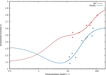
Figure 2.Entrainment functionsA(zs)for jets and plumes
depend-ing on the dimensionless heightzs=z/2ro. Functions have been
obtained by fitting experimental data (points) from Carazzo et al. (2006) (forzs>10) and multiplying by a correction function (20c) to extend the functions tozs<10 verifying function continuity and convergence to values ofA=1.11 for jets andA=1.31 for plumes whenzs→0.
Table 3.Constants defining the entrainment functions for jets and
plumes following the formulation introduced by Kaminski et al. (2005) (see Eq. 20a to 20c) obtained after fitting experimental data reported in Carazzo et al. (2006). For Kaminski-R we considered all data including that of Rouse et al. (1952), whereas for Kaminski-C, as suggested by Carazzo et al. (2006), data from Rouse et al. (1952) was excluded.
Kaminski-R Kaminski-C jets plumes jets plumes
c0 1.92 1.61717 1.92 1.55
c1 3737.26 478.374 3737.26 329.0 c2 4825.98 738.348 4825.98 504.5 c3=2(c2−c1) 2177.44 519.948 1883.81 351.0 c4 0.00235 -0.00145 0.00235 −0.00145
2.3 Modelling of the umbrella region
The umbrella region is defined as the upper region of the plume, from about the NBL to the top of the column. This re-gion can be dominated by fountaining processes of the erup-tive mixture that reaches the top of the column, dissipating the excess of momentum at the NBL, and then collapsing as a gravity current (e.g. Woods and Kienle, 1994; Costa et al., 2013). The 1-D BPT should not be extended to this region because it assumes that the mixture still entrains air with the same mechanisms as below NBL and, moreover, predicts that the radius goes to infinity towards the top of the column. For these reasons, we describe the umbrella region adopting a simple semi-empirical approximation.
mix-ture is homogeneous, i.e. the content of air, water vapour, liquid water, ice and total mass of particles do not vary with z. PressureP (z)is considered equal to the atmospheric pres-surePa(z)evaluated at the same level, whereas temperature decreases withzdue to the adiabatic cooling:
P (z)=Pa(z)and dT dP =
1
ˆ
cρˆ. (22)
As a consequence, the density of the mixture varies accord-ingly. The total height of the volcanic plumeHt, above the
vent, is approximated as (e.g. Sparks, 1986)
Ht=cH(Hb+8ro), (23)
where cH is a dimensionless parameter (typically cH=
1.32),Hbis the height of the neutral buoyancy level (above the vent) androthe radius at the vent. BetweenHbandHt,
the coordinatesx andy of the position of the plume centre and the plume radius r are parameterized as a function of the elevationz, withHb≤z≤Ht. The position of the plume
centre is assumed to vary linearly with the same slope at the NBL, whereas the effective plume radius is assumed to de-crease as a Gaussian function:
x=xb+(z−Hb) dx dz
z=zb
, (24)
y=yb+(z−Hb) dy dz
z=zb
, (25)
r=rbe−(z−Hb) 2/2σ2
H, (26)
wherexb,yb,rbare, respectively, the coordinatesxandyof
the centre of the plume and the plume radius at the NBL, and σH =Ht−Hb.
Finally, assuming that the kinetic energy of the mixture is converted to potential energy, the vertical velocity is approx-imated to decrease as the square root of the distance from the NBL:
uz=uzb
s
Ht−z
Ht−Hb
, (27)
whereuzbis the vertical velocity of the plume at the NBL. Although the proposed empirical parameterization of the re-gion above the NBL is qualitatively consistent with the trends predicted by 3-D numerical models (Costa et al., 2015), a more rigorous description requires further research.
3 Plume wet aggregation model
Particle aggregation can occur inside the column or in the ash cloud during subsequent atmospheric dispersion (e.g. Carey and Sigurdsson, 1982; Durant et al., 2009), thereby affecting the sedimentation dynamics and deposition of volcanic ash. Our model explicitly accounts for aggregation in the plume
by adding source (A+i ) and sink (A−i ) terms for aggregates and aggregated particles in their respective particle mass bal-ance Eqs. (2g) and by modifying the settling velocity of ag-gregates. Given the complexity of aggregation phenomena, not yet fully understood, we consider only the occurrence of wet aggregation and neglect dry aggregation mechanisms driven by electrostatic forces or disaggregation processes re-sulting from particle collisions that can break and decom-pose aggregates. Costa et al. (2010) and Folch et al. (2010) proposed a simplified wet aggregation model in which par-ticles aggregate on a single effective aggregated class char-acterized by a diameterdA (i.e. aggregation only involves particle classes having an effective diameter smaller thandA, typically in the range 100–300 µm). Obviously the assump-tion that all particles aggregate into a single particle class is simplistic and considering a range of aggregating classes would be more realistic. However, there are no quantitative data available for such a calibration. Hence, considering this assumption it follows that
A+i =
n X
j=k+1
A−jδik, (28)
wherekis the (given) index of the aggregated class and the sum overj spans all particle classes having diameters lower thandA. The mass of particles of classi (di< dA) that
ag-gregate per unit of time and length in a given plume cross section is
A−i = ˙ni
ρpi
π 6d
3
i
π r2, (29)
wheren˙i is the number of particles of classithat aggregate
per unit volume and time, estimated as
˙
ni≈ ˙
ntotNi P
Nj
. (30)
In the expression above, Ni is the number of particles of
diameterdi in an aggregate of diameterdA, andntot˙ is the
total particle decay per unit volume and time. Costa et al. (2010) considered thatNiis given by a semi-empirical fractal
relationship (e.g. Jullien and Botet, 1987; Frenklach, 2002; Xiong and Friedlander, 2001):
Ni=kf d
A di
Df
, (31)
wherekf is a fractal pre-factor andDf is the fractal
expo-nent. Costa et al. (2010) and Folch et al. (2010) assumed constant values forkf andDf that were calibrated by
distribution to include micrometric and sub-micrometric par-ticles, for which the Brownian kernel is the dominant one (it is known that Brownian particle–particle interaction has typical values of Df ≈2, with values ranging between 1.5
and 2.5, e.g. Xiong and Friedlander, 2001). Actually, prelimi-nary model tests involving micrometric and sub-micrometric particle classes considering constant values forDf andkf
have revealed a strong dependency of results (fraction of ag-gregated mass) on both granulometric cut-off and bin width (particle grain size discretization). In order to overcome this problem, we assume a size-dependent fractal exponent as Df(d)=Dfo−
a (Dfo−Dmin) 1+exp((d−dµ) / dµ)
, (32)
where Df o≤3, Dmin=1.6, dµ≈2µm and a=1.36788.
The values ofDminanddµrepresent, respectively, the
mini-mum value ofDf relevant for sub-micrometric particles and
the scale below which the Brownian aggregation kernel be-comes dominant. For the fractal pre-factorkf we adopt the
expression of Gmachowski (2002):
kf = "r
1.56−(1.728−Df
2 ) 2
−0.228
#Df 2+Df
Df
Df/2 .
(33) Figure 4 shows the values ofDf(d)andkf(d)predicted by
Eqs. (32) and (33) for a range ofDf o. We have performed
different tests to verify that, in this way, the results of the aggregation model become much more robust independently of the distribution cut-off (8min=8,10,12) and bin width (18=1,0.5,0.25), with maximum differences in the aggre-gated mass laying always below 10 %.
The total particle decay per unit volume and time n˙tot is given by
˙
ntot= ˆf αm(ABntot2 +ATIφ4/ Dfn 2−4/ Df tot
+ASφ3/ Dfn
2−3/Df
tot +ADSφ4/ Dfn 2−4/ Df
tot ), (34)
whereαm is a mean (class-averaged) sticking efficiency, φ is the solid volume fraction,ntot is the total number of par-ticles per unit of volume that can potentially aggregate and
ˆ
f is a correction factor that accounts for conversion from Gaussian to top-hat formalism (see Appendix A for details). The expression above comes from integrating the collection kernel over all particle sizes, and involves the product of the (averaged) sticking efficiency times the collision frequency function accounting for Brownian motion (AB), collision due to turbulence as a result of inertial effects (ATI), laminar and turbulent fluid shear (AS), and differential sedimentation (ADS). The termABderives from the Brownian collision ker-nelβB,ij (Costa et al., 2010):
βB,ij=
2kbTˆ 3µˆ
(di+dj)2
djdj
, (35)
!"#$
!%#$
0 20 40 60 80 100
0 0.1 0.2 0.3 0.4 0.5 0.6 0.7 0.8 0.9 1 1.1 0 0.5 1 1.5 2 2.5 3 3.5 4
Dimensionless height z_s
Height (km a.v.l.)
Entrainment coefficients Jet region
Plume region Umbrella region
a_s a_v
0 5 10 15 20 25 30
0 0.1 0.2 0.3 0.4 0.5 0.6 0.7 0.8 0.9 1 1.1 0 5 10 15 20 25 30 35
Dimensionless height z_s
Height (km a.v.l.)
Entrainment coefficients Jet region
Plume region Umbrella region
a_s a_v
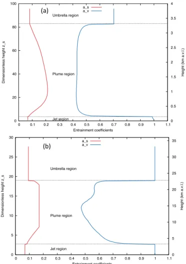
Figure 3.Entrainment coefficientsαs (red) andαv (blue) versus
height for weak(a)and strong (b)plumes under a wind profile. The vertical dashed lines indicate the transition between the differ-ent eruptive column regions. Weak plume simulation with:Mˆo=
1.5×10⁶kgs−1,uˆo=135 ms−1,Tˆo=1273 K,xˆwo=0.03. Strong
plume simulation with: Mˆo=1.5×10⁹kg s−1, uˆo=300 ms−1, ˆ
To=1153 K,xˆwo=0.05.
wherekbis the Boltzmann constant andµˆ is the mixture dy-namic viscosity (≈air viscosity at the bulk temperatureTˆ). The termATIderives from the collision kernel due to turbu-lence as result of inertial effectsβTI,ij (e.g. Pruppacher and
Klett, 1996; Jacobson, 2005): βTI,ij=
ǫ3/4 gνˆ1/4
π
4(di+dj) 2
|usj−usi|, (36)
whereνˆ is the mixture kinematic viscosity andǫis the dis-sipation rate of turbulent kinetic energy, computed assuming the Smagorinsky–Lilly model:
ǫ=2√2k2s ˆ u3
r , (37)
turbulent fluid shearβS,ij (Costa et al., 2010):
βS,ij =
ŴS
6 di+dj
3
, (38)
whereŴS is the fluid shear, computed as
ŴS=max
duˆ dr
,ǫ ν
1/2
. (39)
Finally, the termADSderives from the differential sedimen-tation collision kernelβDS,ij (e.g. Costa et al., 2010):
βDS,ij=
π
4(di+dj) 2
|usi−usj|, (40)
where usi denotes the settling velocity of particle class i.
Note that, with respect to the original formulation of Costa et al. (2010), using the same approach and approximation, we have included the additional termATIdue to the turbulent inertial kernel that, thanks to the similarity between Eqs. (40) and (36), can be easily derived. Once these kernels are inte-grated, expressions for the terms in Eq. (34) yield
AB= − 4kbTˆ
3µˆ , (41a)
AS= −
2 3ŴSξ
3,
(41b)
ADS= −
π(ρp− ˆρ)gξ4
48µˆ , (41c)
ATI=1.82 ǫ3/4
gν1/4ADS, (41d)
whereξ=djv−
1/Df
j is the diameter to volume fractal
rela-tionship andvjis the particle volume. Note that for spherical
particles in the Euclidean space (Df =3) vj=π dj3/6 and
ξ =(6/π )1/3.
The total number of particles per unit of volume available for aggregation is related to particle class mass concentration at each section of the plumeCˆj and can be estimated as (see
Appendix B)
ntot= 1 3 log 2
X
j
6Cˆj
π 18jρpj ! "
1 daj3 −
1 dbj3
#
, (42)
wheredaj anddbj are the particle diameters of the limits of
the intervaljand
ˆ
Cj= ˆρ ˆ
Mj ˆ
M. (43)
Finally, the class-averaged sticking efficiencyαmappearing in Eq. (34) is computed as
αm=
P i
P
jfifjαij P
i P
jfifj
, (44)
wherefk is the particle class mass fraction, andαij is the
sticking efficiency between the classesiandj. In presence of a pure ice phase we assume that ash particles stick as ice par-ticles (αm=0.09). In contrast, in presence of a liquid phase, the aggregation model considers
αij=
1 1+(Stij/ Stcr)q
, (45)
whereStcr=1.3 is the critical Stokes number,q=0.8 is a constant, andStij is the Stokes number based on the binder
liquid (water) viscosity: Stij=
8ρˆ
9µl didj
di+dj|
ui−uj|, (46)
where
|ui−uj| = |usi−usj| +
8kbTˆ 3µπ dˆ idj +
2Ŵs(di+dj)
3π . (47)
Obviously, our aggregation model requires the presence of water either in liquid or solid phases, i.e. aggregation will only occur in those regions of the plume where water vapour (of magmatic origin or entrained by moist air) meets con-densation/deposition conditions (Costa et al., 2010; Folch et al., 2010). This depends on complex relationships be-tween plume dynamics and ambient conditions. For high-intensity (strong) plumes having high values ofM, the con-ˆ ditionPv≥elwhenT > Tˆ f is rarely met, implying no
for-mation of a liquid water window within the plume. Aggre-gation occurs in this case only at the upper parts of the col-umn, under the presence of ice. In contrast, lower-intensity (weak) plumes having lower values ofMˆ can form a liquid water window if the termMa dominates in Eq. (8a). How-ever, this also depends on a complex balance between air en-trainment efficiency, ambient moisture, plume temperature, height level, cooling rate and ambient conditions. Aggrega-tion by liquid water is much favoured under moist environ-ments and by efficient air entrainment. Note that, keeping all eruptive parameters constant, the occurrence (or not) of wet aggregation by liquid water can vary with time depending on fluctuations of the atmospheric moisture and wind intensity along the day.
4 FPLUME-1.0
vent coordinates (xo,yo) and elevation (zo), conditions at the
vent (exit velocityuˆo, magma temperatureTˆo, magmatic
wa-ter mass fraction wˆo, and total grain size distribution) and
total column heightHt or mass eruption rateMˆo. The code
has two solving modes. If Mˆo is given, the code solves
di-rectly forHt. On the contrary, ifHt is given, the code solves
iteratively forM. Wind profiles can be furnished in differentˆ formats, including standard atmosphere, atmospheric sound-ings, and profiles extracted from meteorological re-analysis data sets. If the aggregation model is switched on, additional inputs are required including size and density of the aggre-gated class, aggregates settling velocity factor (to account for the decrease in settling velocity of aggregates due to increase in porosity), and fractal exponent for coarse particles Df o.
The rest of the parameters (specific heats, the value of the constant χ for particle fallout probability, parameterization of the entrainment coefficients, etc.) have assigned default values but can be modified by the user using a configure file. Model outputs include a text file with the results for each eruption phase giving values of all computed variables (e.g.
ˆ
u,Tˆ,ρ) at different heights, and a file giving the mass flowˆ
rate of each particle class that falls from the column at dif-ferent heights (cross sections). This file provides the phase-dependent source term, and hence serves to couple FPLUME with atmospheric dispersion models. In case of wet aggre-gation, the effective granulometry predicted by the aggrega-tion model is also provided. The soluaggrega-tion of the aggregaaggrega-tion model embedded in FPLUME-1.0 consists on the following steps:
1. At each section of the plume, determine the water vapour condensation or deposition conditions depend-ing onTˆ andPvusing Eqs. (11) or (12), respectively. 2. In case of saturation or deposition, compute the
class-averaged sticking efficiencyαmfor liquid water or ice using Eq. (44).
3. Estimate the total number of particles per unit of vol-ume available for aggregationntotdepending onCˆj
us-ing Eq. (42).
4. Compute the integrated aggregation kernels using Eq. (41a) to (41d).
5. Compute the total particle decay per unit volume and timen˙totusing Eq. (34) depending also on the solid vol-ume fraction.
6. Compute the number of particles of diameterdi in an
aggregate of given diameterdAusing Eq. (31) assuming size-dependent fractal exponentDf and pre-factorkf.
7. Compute class particle decayn˙i using Eq. (30).
8. Finally, compute the mass sink term for each aggregat-ing classA−i using Eq. (29) and the mass source term A+i for the aggregated class using Eq. (28) to introduce
these terms in the particle class mass balance equations, Eq. (2g).
5 Test cases
As we mentioned above, here we apply FPLUME to two eruptions relatively well characterized by previous studies. In particular we consider the strong plume formed during 4 April 1982 by El Chichón 1982 eruption (e.g. Sigurds-son et al., 1984; Bonasia et al., 2012) and the weak plume formed during the 6 May 2010 Eyjafjallajökull eruption (e.g. Bonadonna et al., 2011; Folch, 2012).
5.1 Phase-B El Chichón 1982 eruption
El Chichón volcano reawakened in 1982 with three signif-icant Plinian episodes occurring during March 29th (phase A) and April 4th (phases B and C). Here we focus on the second major event, starting at 01:35 UTC on April 4th and lasting nearly 4.5 h (Sigurdsson et al., 1984). Bonasia et al. (2012) used analytical (HAZMAP) and numerical (FALL3D) tephra transport models to reconstruct ground deposit obser-vations for the three main eruption fallout units. Deposit best-fit inversion results for phase-B suggested column heights between 28 and 32 km (above vent level, a.v.l.) and a total erupted mass ranging between 2.2×10¹²and 3.7×10¹²kg. Considering a duration of 4.5 h, the resulting averaged mass eruption rates are between 1×10⁸and 2.3×10⁸kg/s. TGSD of phases B and C were estimated by Rose and Durant (2009) weighting by mass, by isopach volume and using the Voronoi method. Bonasia et al. (2012) found that the reconstruction of the deposits is reasonably achieved taking into account the empirical Cornell aggregation parameterization (Cornell et al., 1983). In this simplistic approach, 50 % of the 63– 44 µm ash, 75 % of the 44–31 µm ash and 100 % of the less than 31 µm ash are assumed to aggregate as particles with a diameter of 200 µm and density of 200 kg m−3. Note that here, as in previous studies (Folch et al., 2010), we use a modified version of Cornell et al. (1983) parameterization that assumes that 90 % and not 100 % of the particles smaller than 31 µm fall as aggregates.
Table 4.Input values for the El Chichón Phase-B simulation. Values for specific heat of water vapour, liquid water, ice, pyroclasts and air at constant pressure are assigned to defaults of 1900, 4200, 2000, 1600 and 1000 Jkg−1K−1.
Parameter Symbol Units Value
Phase start h 01:35 UTC
Phase end h 06:00 UTC
Exit velocity uˆo ms−1 350
Exit temperature Tˆo K 1123
Water mass fraction wˆo – 4 %
Diameter aggregates dA µm 250
Density aggregates ρˆA kg m−3 200
Probability of particle fallout χ − 0.23 Shear entrainment coefficient αs – Eq. (19)
Vortex entrainment coefficient αv − Eq. (21)
1 1.2 1.4 1.6 1.8 2 2.2 2.4 2.6 2.8 3 3.2
-6 -5 -4 -3 -2 -1 0 1 2 3 4 5 6 7 8 9 10 11
Fractal exponent D
f
Φ-number
Dfo=3.0 Dfo=2.9 Dfo=2.8
Figure 4.Dependency of fractal exponentDf (continuous lines)
and fractal pre-factorkf (dashed lines) on particle size expressed in
8units according to Eq. (32) and (33) for different values ofDf o.
Note the progressive decay inDfstarting at8=7 (d≈10 µm) and
leading to values ofDf =1.6 for8=9 (d≈2µm).
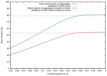
(a.s.l.), a mass eruption rate of 2.7×10⁸kg s−1 and a total erupted mass of 4.4×10¹²kg. These values are consistent but slightly higher than those from previous studies (Bona-sia et al., 2012). Regarding the aggregation model, we did several sensitivity runs to look into the impact of the frac-tal exponentDf oon the fraction of aggregates, ranging this
parameter between 2.85 and 3.0 at 0.01 steps values (see Fig. 6). As anticipated in the original formulation (Costa et al., 2010; Folch et al., 2010), the results of the aggregation model are sensitive to this parameter. Values ofDf o=2.96
fit very well the total mass fraction of aggregates predicted by Cornell but not the fraction of the aggregating classes (Fig. 7b). In contrast, we find a more reasonable fit with Df o=2.92, although in this case the relative differences for
the total mass fraction of aggregates are of about 15 %, with our model under-predicting with respect to Cornell (Fig. 7a).
0 5 10 15 20 25 30 35
0 5 10 15 20 25 30
-80 -70 -60 -50 -40 -30 -20 -10 0 10 20 30 40
Height (km a.s.l.)
Wind Speed (m/s) Temperature (C)
Wind speed Temperature
0 5 10 15 20 25 30
0 2 4 6 8 10 12 5 10 15 20 25 30 0 50 100 150 200 250 300 350
Height (km above the vent)
Height (km a.s.l.)
Plume radius (km) Plume velocity (m/s)
Plume radius Plume velocity NBL
!"#$
!%#$
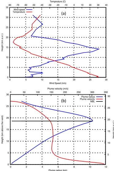
Figure 5. (a): wind and temperature atmospheric profiles during 4
April 1982 at 00:00 UTC from sounding.(b): FPLUME bulk veloc-ityuˆ and radiusrwith heightz. The black solid line indicates the height of the NBL determined by the model.
A clear advantage of a physical aggregation model of ash particles inside the eruption column, with respect to an em-pirical parameterization like Cornell et al. (1983), is that it al-lows for estimating the fraction of very fine ash that escapes to aggregation processes and is transported distally within the cloud. As we mentioned above, based on the features of the observed deposits, Cornell et al. (1983) proposed that 100% of particles smaller than 31 µm fall as aggregates, which is quite reasonable as most of fine ash falls prematurely. How-ever assessing the small mass fraction of fine ash that escapes to aggregation processes is crucial for aviation risk mitiga-tion and for comparing model simulamitiga-tions with satellite ob-servations. For example, in the case of El Chichón 1982 erup-tion, forDf o=2.92, the model predicts that≈10% of fine
0 10 20 30 40 50 60 70 80 90 100
2.85 2.86 2.87 2.88 2.89 2.9 2.91 2.92 2.93 2.94 2.95 2.96 2.97 2.98 2.99 3
Mass fraction (%)
Fractal exponent D_fo Total mass fraction of aggregates
Modifyed Cornell model Mass fraction of aggregates (respect to fines) Modifyed Cornell model (respect to fines)
Figure 6.El Chichón 1982 phase-B simulation. Total mass fraction
of aggregates (red line) and total mass fraction of aggregates with respect to fines (blue line), depending on the fractal exponentDf o.
The (constant) values predicted by the modified Cornell model are shown by dashed lines.
High Resolution Radiometer (AVHRR) data, but we need to consider that we do not account for dry aggregation that can be dominant for very fine particles.
5.2 6 May 2010 Eyjafjallajökull eruption phase
The infamous April–May 2010 Eyjafjallajökull eruption, that disrupted the European North Atlantic region airspace (e.g. Folch, 2012), was characterized by a very pulsating be-haviour, resulting on nearly continuous production of weak plumes that oscillated on height between 2 and 10 km (a.s.l.) during the 39-day-long eruption (e.g. Gudmundsson et al., 2012). During 4-8 May, Bonadonna et al. (2011) per-formed in situ observations of tephra accumulation rates and PLUDIX Doppler radar measurements of settling velocities at different locations, which then used to determine erupted mass, mass eruption rates and grain size distributions. The authors estimated a TGSD representative of 30 min of erup-tion by combining ground-based grain-size observaerup-tions (us-ing a Voronoi tessellation technique) and ash mass retrievals (7-98particles) from MSG-SEVIRI satellite imagery for 6 May between 11:00 and 11:30 UTC. On the other hand, they also report the in situ observation of sedimentation of dry and wet aggregates falling as particle clusters and poorly structured and liquid accretionary pellets (AP1 and AP3 ac-cording to Brown et al. (2012) nomenclature). Bonadonna et al. (2011) did also grain-size analyses of collected ag-gregates using scanning electron microscope (SEM) images. The combination of all these data allowed them to determine how the original TGSD was modified by the formation of dif-ferent types of aggregates (see Fig. 8). The total mass fraction of aggregates was estimated to be about 25% with aggregate sizes ranging between 18(500 µm) and 48(62.5 µm). These
0 5 10 15 20 25 30 35 40 45 50 55
-7 -6 -5 -4 -3 -2 -1 0 1 2 3 4 5 6 7 8 9 10 11 128000 64000 32000 16000 8000 4000 2000 1000 500 250 125 62.5 31.2 15.6 7.8 3.9 1.9 0.9 0.4
Mass fraction (%)
!-number Diameter (µm)
Aggregation model Original TGSD Modified Cornell aggregation model
0 5 10 15 20 25 30 35 40 45 50 55
-7 -6 -5 -4 -3 -2 -1 0 1 2 3 4 5 6 7 8 9 10 11 128000 64000 32000 16000 8000 4000 2000 1000 500 250 125 62.5 31.2 15.6 7.8 3.9 1.9 0.9 0.4
Mass fraction (%)
!-number Diameter (µm)
Aggregation model Original TGSD Modified Cornell aggregation model !"#$
!%#$
Figure 7.Results of the aggregation model in FPLUME for El
Chichón 1982 phase-B simulation. Green bars show the original TGSD from Rose and Durant (2009) discretized in 178-classes. Blue bars show the results of the modified Cornell model. Finally, read bars give the results of our wet aggregation model considering a fractal exponent ofDf o=2.92(a)andDf o=2.96(b).
results constitute a rare and valuable data set to test the ag-gregation model implemented in FPLUME. However, sev-eral challenges can be anticipated. First, our model assumes a single aggregated class and, as a consequence, we may ex-pect to reproduce only the total mass fraction of aggregates, but not to match the resulting mass fraction distribution class by class. Second, the proportion of dry versus wet aggre-gates is unknown and, wet aggregation could have occurred within the plume but also by local rain showers that scav-enged coarse particles (Bonadonna et al., 2011); moreover, the presence of meteoritic water in the plume (not consid-ered here) could significantly enhance aggregation. For these reasons, we aim to capture the correct order of magnitude of total mass fraction of ash that went into aggregates.
0 2 4 6 8 10 12 14 16 18 20 22 24 26 28
-3 -2 -1 0 1 2 3 4 5 6 7 8 9 10
8000 4000 2000 1000 500 250 125 62.5 31.2 15.6 7.8 3.9 1.9 0.9
Mass fraction (%)
Φ-number Diameter (µm)
Aggregates Ground+MSG SEVIRI
Figure 8. Original grain size distribution from ground data and
MSG-SEVIRI retrievals (green) and distribution modified by ag-gregation (red). Results are for 6 May 30 min averaged. Figure re-produced from Bonadonna et al. (2011) (Fig.17d).
Table 5.FPLUME input values for the 6 May Eyjafjallajökull
sim-ulation. Values for specific heats of water vapour, liquid water, ice, pyroclasts and air at constant pressure are assigned to defaults of 1900, 4200, 2000, 1600 and 1000 Jkg−1K−1.
Parameter Symbol Units Value
Phase start h 06:00 UTC
Phase end h 12:00 UTC
Exit velocity uˆo ms−1 150
Exit temperature Tˆo K 1200
Water mass fraction wˆo − 3 %
Diameter aggregates dA µm 500 Density aggregates ρˆA kg m−3 200
Probability of particle fallout χ – 0.23 Shear entrainment coefficient αs – Eq. (19)
Vortex entrainment coefficient αv – Eq. (21)
of a liquid water window nor the formation of ice. However, on short timescales these plume heights are very different from the daily (hourly) time-averaged values. In fact, Arason et al. (2011) determined a 5 min time series of the echo-top radar data of the eruption plume altitude and for 6 May they observed oscillations between 3.5 and 8.5 km (a.v.l). This is consistent with Gudmundsson et al. (2012), who for 6 May reported a median plume height of 4 km (a.v.l.) and a maxi-mum elevation of around 8 km (a.v.l.). This may suggest that wet aggregates could have formed within the plume not con-tinuously but during sporadic higher-intensity column pulses. In order to check this possibility, we performed a parametric study to compute the total mass fraction of wet aggregates as function of mass flow rate that controls the value of the column height.
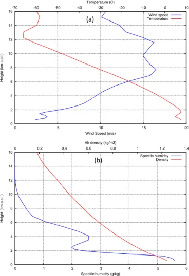
Input values for FPLUME are summarized in Table 5. The wind profile (see Fig. 9) was extracted from the ERA-Interim re-analysis data set interpolating values at the vent
0 2 4 6 8 10 12 14 16
0 5 10 15 20
-70 -60 -50 -40 -30 -20 -10 0 10
Height (km a.s.l.)
Wind Speed (m/s) Temperature (C)
Wind speed Temperature
0 2 4 6 8 10 12 14 16
0 1 2 3 4 5 6
0 0.2 0.4 0.6 0.8 1 1.2 1.4
Height (km a.s.l.)
Specific humidity (g/kg) Air density (kg/m3)
Specific humidity Density !"#$
!%#$
Figure 9. Atmospheric profiles extracted form ERA-Interim
re-analysis data set at Eyjafjallajökull vent location for 6 May 2010 at 12:00 UTC.(a): wind and temperature profiles.(b): specific hu-midity and air density profiles.
nates. As shown in Fig. 10, 10 % in mass of wet aggregates is predicted by our model for column heights ranging between 6 and 7 km (a.v.l.) and 20% for column heights from 7.2 to 8.3 km (a.v.l.). For the considered input parameters and am-bient conditions (wind and moisture profile), we observed the formation of a window in the plume containing liquid water only for column heights above 5.3 km (a.v.l.). For illustrative purposes, Fig.11 shows the resulting grain size distribution for a column height of 6.5 km (a.v.l.) and two different val-ues of the fractal exponentDf. As anticipated, the model
0 2 4 6 8 10 12 14 16 18 20 22 24 26 28 30
0.5 1 1.5 2 2.5
4.5 5 5.5 6 6.5 7 7.5 8 8.5
Mass fraction aggregates (%)
Mass Flow Rate (x 1e6 kg/s) Column height (km a.v.l)
D_f = 2.95 D_f = 2.97 D_f = 2.99
Figure 10.FPLUME aggregation model results for Eyjafjallajökull
6 May phase. Total mass fraction of aggregates (in %) versus mass flow rate (in kg s−1) and column height (in km a.v.l.) for different values of the fractal exponentDf o (in these simulations we used
cH=1.1 and the presence of meteoritic water in the plume was not
considered). The model predicts a 10 % in mass of wet aggregates for column heights between 6.0 and 7.0 km (a.v.l.). Input parameters were fixed as in Table 5 varying mass flow rate (column height).
0 2 4 6 8 10 12 14 16 18 20 22 24 26 28 30 32 34 36 38 40
-3 -2 -1 0 1 2 3 4 5 6 7 8 9 10
8000 4000 2000 1000 500 250 125 62.5 31.2 15.6 7.8 3.9 1.9 0.9
Mass fraction (%)
Φ-number Diameter (µm)
Observed FPLUME Df=2.95 FPLUME Df=2.99
Figure 11. Grain size distribution predicted by the wet
aggrega-tion model for Eyjafjallajökull 6 May phase for a column height of 6.5 km (a.v.l.) for two different values of the fractal exponentDf o
of 2.95 and 2.99. Observed data from Bonadonna et al. (2011).
6 Conclusions
We presented FPLUME, a 1-D cross-section-averaged vol-canic plume model based on the BPT that accounts for plume bending by wind, entrainment of ambient moisture, effects of water phase changes, particle fallout and re-entrainment, a new parameterization for the air entrainment coefficients and an ash wet aggregation model based on Costa et al. (2010). Given conditions at the vent (mixture exit velocity,
temper-ature and magmatic water content) and a wind profile, the model can solve for plume height given the eruption rate or vice versa. FPLUME can also be extended above the NBL, i.e. to solve the umbrella region semi-empirically in case of strong plumes. In case of favourable wet aggregation condi-tions (formation of a liquid water window inside the plume or in presence of ice at the upper regions), the aggregation model predicts aneffectivegrain size distribution consider-ing a sconsider-ingle aggregated class. For the aggregation model, two test cases have been considered, the Phase-B of El Chichón 1982 eruption and the 6 May 2010 Eyjafjallajökull eruption phase. For the first case, we got reasonable agreement with the empirical Cornell parameterization using a fractal expo-nent ofDf o=2.92, with wet aggregation occurring under
the presence of ice (as expected for large strong plumes). For the second case, we could reproduce the observed to-tal mass fraction of aggregates for plume heights between 6.7 and 8.5 km (a.v.l.). Wet aggregation occurs in this case within a narrow window where conditions for liquid water to form are met. In case of aggregation, results are sensitive to the fractal exponent, which may range fromDf o=2.92
toDf o=2.99. Future studies are necessary to better
under-stand and constrain the role of this parameter.
Code availability
Appendix A: Correction factorfˆfor mass distribution for top-hat versus Gaussian formalism
Denoting withR the top-hat radius of the plume and withb the Gaussian length scale the relationship between them can be written as (e.g. Davidson, 1986)
b2=R2/2. (A1)
Assuming a Gaussian profile for the concentration,C(r), the mean value betweenr=0 (where the concentration is max-imum) andr=Ris
hCi =C0/R2 ∞
Z
0
rexp(−r2/b2)dr=
C0/(2b2) ∞
Z
0
rexp(−r2/b2)dr=0.25C0 (A2)
that impliesCˆ =0.25C0. Following similar calculations we have also
hC2i =C02/R2 ∞
Z
0
rexp(−2r2/b2)dr=
C02/(2b2) ∞
Z
0
rexp(−2r2/b2)dr=0.125C02, (A3)
hC3i =C03/R2 ∞
Z
0
rexp(−3r2/b2)dr=
C03/(2b2) ∞
Z
0
rexp(−3r2/b2)dr=0.0833C03. (A4)
Therefore, if we use average (top-hat) variables in Eq. (34) we need to keep in mind that concentration appears in the nonlinear terms and therefore we should use the following correction factors:
ˆ
f2=h C2i
ˆ
C2 =
0.125C02 (0.25C0)2=
0.125C02
0.0625C02=2, (A5)
ˆ
f3=hC 3i
ˆ
C3 =
0.0833C02
0.015625C03 =5.33, (A6)
and so on (h·idenotes the average using the top-hat filter, e.g.
ˆ
C= hCi). Because terms in Eq. (34) scale with concentra-tion with a power of two we need to account for a correcconcentra-tion factorfˆ= ˆf2. The factorfˆcan be also used to correct un-derestimation of Eulerian timescale with respect Lagrangian timescale (e.g. Dosio et al., 2005).
Appendix B: Computation ofntot
Consider a particle grain size distribution discretized in n bins of width 18j with the bin centre at 8j and where
8j aand8j bare the bin limits (i.e.18j=8j b−8j a). The
number of particles per unit volume in the bin8j (assuming
spherical particles) is
n(8j)= 8j b
Z
8j a
6C(8)
πρ(8)d3(8)d8. (B1)
Considering that d(8)=d∗2−8=d
∗e−8log 2 and the top-hat formalism, the above expression can be approached as
n(8j)≈
6Cˆj
π ρjd∗318j 8j b
Z
8j a
e38log 2d8
= 1
3 log 2
6Cˆj
π ρjd∗318j !
h
e3 log 28j b−e3 log 28j ai. (B2)
Adding the contribution of all bins, this yields to
ntot= 1 3 log 2d3
∗
X
j
6Cˆj
π ρj18j !
h
e3 log 2(8j+18j/2)−e3 log 2(8j−18j/2)i (B3) or, in terms of particle diameter,
ntot= 1 3 log 2
X
j
6Cˆj
π 18jρj ! "
1 daj3 −
1 dbj3
#
, (B4)