www.atmos-chem-phys.net/10/8917/2010/ doi:10.5194/acp-10-8917-2010
© Author(s) 2010. CC Attribution 3.0 License.
Chemistry
and Physics
Development and application of a reactive plume-in-grid model:
evaluation over Greater Paris
I. Korsakissok1,2and V. Mallet2,1
1CEREA, Joint Research Laboratory, ENPC/EDF R&D, Universit´e Paris Est, 6–8 avenue Blaise Pascal, Cit´e Descartes, 77455 Champs-sur-Marne, Marne la Vall´ee Cedex 2, France
2INRIA, Paris-Rocquencourt Research Center, B.P. 105, 78153 Le Chesnay Cedex, France Received: 5 February 2010 – Published in Atmos. Chem. Phys. Discuss.: 22 February 2010 Revised: 23 June 2010 – Accepted: 6 September 2010 – Published: 22 September 2010
Abstract.Emissions from major point sources are badly rep-resented by classical Eulerian models. An overestimation of the horizontal plume dilution, a bad representation of the ver-tical diffusion as well as an incorrect estimate of the chemical reaction rates are the main limitations of such models in the vicinity of major point sources. The plume-in-grid method is a multiscale modeling technique that couples a local-scale Gaussian puff model with an Eulerian model in order to bet-ter represent these emissions. We present the plume-in-grid model developed in the air quality modeling system Polyphe-mus, with full gaseous chemistry. The model is evaluated on the metropolitan ˆIle-de-France region, during six months (summer 2001). The subgrid-scale treatment is used for 89 major point sources, a selection based on the emission rates of NOxand SO2. Results with and without the subgrid treat-ment of point emissions are compared, and their performance by comparison to the observations on measurement stations is assessed. A sensitivity study is also carried out, on sev-eral local-scale parameters as well as on the vertical diffusion within the urban area.
Primary pollutants are shown to be the most impacted by the plume-in-grid treatment. SO2is the most impacted pollu-tant, since the point sources account for an important part of the total SO2emissions, whereas NOxemissions are mostly due to traffic. The spatial impact of the subgrid treatment is localized in the vicinity of the sources, especially for re-active species (NOxand O3). Ozone is mostly sensitive to the time step between two puff emissions which influences the in-plume chemical reactions, whereas the almost-passive species SO2 is more sensitive to the injection time, which determines the duration of the subgrid-scale treatment.
Correspondence to:I. Korsakissok ([email protected])
Future developments include an extension to handle aerosol chemistry, and an application to the modeling of line sources in order to use the subgrid treatment with road emis-sions. The latter is expected to lead to more striking results, due to the importance of traffic emissions for the pollutants of interest.
1 Introduction
employed here has been developed on the air quality mod-eling system Polyphemus (Mallet et al., 2007). The aim is to provide an easy-to-use, modular model, fit for applica-tions from regional to continental scales, and both for reac-tive and non-reacreac-tive pollutants. It was already described and applied at continental scale for passive tracers (Korsakissok and Mallet, 2010). The model has been extended to han-dle full gaseous chemistry, and is therefore evaluated in this study for photochemical applications.
The chosen application domain is the metropolitan ˆIle-de-France region, with Paris at the center of the domain. Re-gional air quality modeling focused on large urban areas is an important topic, both for decision support (e.g., for emis-sion abatement policies) and to assess impact on health and ecosystems. ˆIle-de-France contains many point source emis-sions, mainly industrial stacks. This application is somewhat different from previous plume-in-grid studies: the model-ing domain is smaller and there is a higher number of point sources (89), but with lower emission rates. For instance, in Vijayaraghavan et al. (2006), the application domain was California. The 10 major point sources selected for the appli-cation emitted slightly more NOxemission rate than the 89 point sources retained here. In our case, the simulations are carried out for six months, during summer 2001. Our anal-ysis is based on both on global results for the whole period, and on a few selected days of interest. This approach dif-fers from that of many other studies, where only some short ozone episodes were selected.
The aim of the study is (1) to determine the plume-in-grid impact, in terms of statistics as well as spatial variability, in the case of a high number of point sources well distributed over an urban area, and (2) to give insights on the sensitivity to various parameters, and on the relevant spatial and tempo-ral scales. Section 2 describes the plume-in-grid model, with an emphasis on the chemistry within the puffs, and Sect. 3 details the application domain and the modeling set-up. In Sect. 4, the plume-in-grid impact is assessed, both on per-formance indicators and in terms of spatial variability. In Sect. 5, we present a sensitivity analysis, focused on the im-pact of the vertical diffusion and on the influence of temporal parameters.
2 Model overview
The plume-in-grid model presented here couples, on the Polyphemus platform, the Gaussian puff model (Korsakissok and Mallet, 2009) with the Eulerian model Polair3D (Bouta-har et al., 2004). It has already been described and evalu-ated for passive tracers at continental scale in Korsakissok and Mallet (2010). In this section, the Gaussian puff model parameterizations, and the coupling method, are only briefly described (Sect. 2.1), with an emphasis on the spatial and temporal scales of the model (Sect. 2.2). We also focus on the description of the chemistry within the puffs (Sect. 2.3).
2.1 Coupling
The Gaussian puff model (Korsakissok and Mallet, 2009) represents a continuous point source emission as a series of puffs with a Gaussian shape in the three directions. Each puff transports a given quantity of each of the emitted species. The puffs move independently from one another, since the speed and direction of a puff are determined by the wind at its center (interpolated from the Eulerian fields). Each puff’s size increases with turbulence, and is determined by the Gaussian standard deviations in all three directions: σx
(downwind),σy (crosswind) andσz(vertical). In the
Gaus-sian puff model of Polyphemus, three empirical parameteri-zations may be used to compute the Gaussian standard devi-ations: Briggs’s, Doury’s and similarity-theory.
In the plume-in-grid model, several point source emissions are treated by the Gaussian puff model while other sources, namely diffuse area emissions, are managed by Polair3D. The two models exchange information at each time step. On one way, background data (meteorological data, concentra-tions, deposition velocities...) is retrieved from the Eulerian model and bi-linearly interpolated at the center of each puff. On the other way, the concentrations handled by the Gaus-sian model are eventually injected into the Eulerian model: the puff’s mass is distributed within the cells vertically cov-ered by the puff.
2.2 Spatial and temporal scales
Two particular temporal scales are focused on, since they are key to the plume-in-grid modeling, and determine the total number of puffs handled by the model at each time step:
– the time step between two puff emissions1tpuff, – the time when a given puff is transferred to the Eulerian
modeltinj.
The full chemical mechanism is applied within each puff, and the computational time increases accordingly. These two pa-rameters have therefore to be chosen carefully, ensuring a reasonable computational time as well as a physically con-sistent modeling. The model sensitivity to these parameters is assessed in Sect. 5, and they are briefly described below. 2.2.1 Time step between two puffs
two successive puffs emitted at timesti andti+1=ti+1tpuff respectively, if:
σx(t−ti)+σx(t−ti+1)≥
u Cy
1tpuff, (1)
whereu is the wind speed at timet and at the puffs’ loca-tions, and the puffs’ standard deviations areσx(t−ti) and σx(t−ti+1)in thex direction. It therefore depends on the meteorological conditions. Cy is the constant which
deter-mines the puffs’ effective size (in practiceCy=2). In the
present case-study, the time step between two puff emissions is1tpuff=100s, to match the Eulerian time step. For a wind speed of 5ms−1, the overlap condition given in Eq. (1) is therefore fulfilled as soon asσx≥125m, which in unstable
conditions is reached within one or two time steps. In stable situations, the puffs’ spread is smaller and the wind speed is lower, so the condition is also fulfilled within a few time steps.
2.2.2 Injection time
The criterion to switch from the local-scale to the Eulerian model (so-called “injection time”) has to be determined so that the artificial dilution due to the Eulerian model is limited, and the Gaussian model error due to trajectory uncertainties is not too large. It depends on the ratio between the Eule-rian cell size and the plume horizontal size, on wind shear, and also on chemistry: for chemically reactive plumes, a puff can be released when its chemical composition does not sig-nificantly differ from the background (Vijayaraghavan et al., 2006). In Korsakissok and Mallet (2010), the influence of the injection time was assessed at several grid resolutions, at continental scale. Two criteria were tested: (1) either the puff is transferred after a given travel time, or puff “age”, called theinjection timetinj, or (2) the puff is transferred as soon has itshorizontal size(given by 2Cy σy) is about the cell size.
The size criterion gave the best results at fine resolution, but the time criterion was better when the grid resolution was too coarse and the puff size criterion would lead to large trans-fer times, inducing large errors in the puffs trajectory. An injection time of the order of magnitude of the time for a puff to cross one cell was suggested, with an upper limit of about three hours. At regional scale, for a mean wind speed of about 5ms−1 and a cell size of 5 km, the injection time would therefore be around 20 minutes, which is used here. This is of the same order of magnitude as the time when the chemical plume regime changes, and becomes closer to the background chemistry (Karamchandani et al., 1998). 2.3 Chemical coupling
Each puff transports all species of the chemical mechanism of the Eulerian model. The initial puff quantities of sec-ondary species are obviously equal to zero. Chemistry takes place in the puffs, with the following characteristics:
– the species in one puffαreact with each other,
– the species of two overlapping puffsαandβreact with each other (Appendix A),
– the species in one puff react with the background species. This interaction is detailed below.
In the case of non-linear chemistry (second order reac-tions), it is necessary to take into account the interaction be-tween the background and the puff species. In the plume-in-grid model, the chemical reactions between the background species are already taken into account in the Eulerian model. Therefore, only the additional perturbation due to the inter-action has to be added to the puff quantity. According to Karamchandani et al. (2000), we use the following procedure 1. Add the background concentrationcbA to the puff centration, and compute the chemistry on the total con-centration. The rate of disappearance for species A, supposing a reaction of typeA+B→P occurs, is then
d(cAα+cbA)
dt = −k(c
α Ac
α B | {z } (1)
+cbAcBb | {z } (2)
+cαAcbB+cαBcbA
| {z }
(3)
), (2)
wherekis the reaction rate, (1) represents the chemistry between the puff species, (2) is the chemistry between the background species, and (3) is the interaction be-tween the puff and background species.
2. Compute separately the chemistry between background species only. The rate of disappearance ofAis then
dcbA
dt = −k c
b
AcBb. (3)
3. Subtract the results of the time integration over one time step of the two previous equations. The term (2) in Eq. (2) is taken into account in the background (Eule-rian) chemistry, and terms (1) and (3) are carried by the puff.
Since the puff carries the interaction term (term (3) in Eq. 2), it can transport negative concentrations. It occurs when a background species, which was not emitted, is de-pleted by a reaction that occurs inside the puff. Thus, the puff can be considered as a “perturbation” to the background con-centration. The total concentration is obtained by adding the puff’s concentration to the background concentration, and is always positive.
0 10 20 30 40 50 60 70 Time after emission (minutes)
-6 -4 -2 0 2 4 6 8
plume mass (micrograms)
x1e+10
NO2 mass
NO mass
O3 mass
Fig. 1.Plume mass in µg for NO2, NO and O3with plume-in-grid. Simulation with one point source of NOxin a uniform background
of O3.
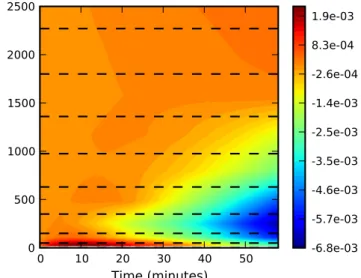
the Eulerian model). Since the puffs carry a perturbation of the background concentrations, the plume mass of O3is negative, and represents the amount of ozone that has been titrated. Although the emitted mass of NO is more than twice that of NO2(emission rates are 21 g s−1and 10 g s−1, respec-tively), the plume mass of NO2is higher after about ten min-utes, due to the titration of O3by NO producing NO2. The source is emitting continuously. After one hour, the puffs are transferred into the Eulerian model, and are no longer in-cluded in the total plume mass, which therefore becomes al-most constant. Figure 2 shows the difference between the O3 concentration profiles, with and without the plume-in-grid treatment for this simple case. O3 concentration is lower within the plume. When using the plume-in-grid model, the NOx plume stays longer above the ground, and is more concentrated, than with the Eulerian model. Thus, using a subgrid-scale treatment induces higher O3 concentrations at ground level in the vicinity of the source, and lower in-plume concentrations. Farther downwind, the in-plume touches the ground, inducing lower ground concentrations with the plume-in-grid model.
3 Application: air quality over Paris region 3.1 Modeling set-up
The plume-in-grid model is applied over Paris region, during 6 months for the year 2001, from 01-04-2001 to 27-09-2001. The simulation set-up is similar to that used in Tombette and Sportisse (2007). The simulation area covers the ˆIle-de-France, and ranges from 1.40◦E to 3.55◦E (44 cells) and from 48.10◦N to 49.20◦N (23 cells) (Fig. 3). The cells size
0
10
20
30
40
50
Time (minutes)
0
500
1000
1500
2000
2500
-6.8e-03
-5.7e-03
-4.6e-03
-3.5e-03
-2.5e-03
-1.4e-03
-2.6e-04
8.3e-04
1.9e-03
Fig. 2.Vertical profile as a function of time: difference between O3
concentrations averaged over the simulation domain (in µg m−3) with and without the subgrid treatment. Simulation with one point source of NOxin a uniform background of O3. The dashed lines
represent the vertical levels interfaces of the Eulerian model. The vertical levels are indicated in meters above the ground.
s23
s32 s25
s24
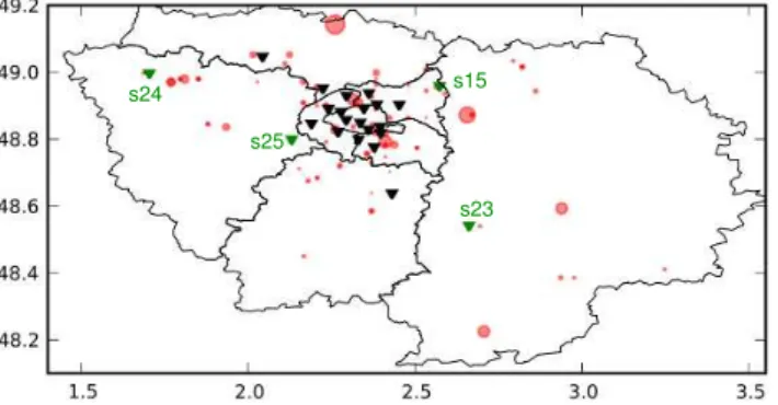
Fig. 3. Measurement stations (triangles), and main point sources, for SO2. The circles areas are proportional to the sources
emis-sion rate. The black triangles are urban stations, green triangles are periurban and rural stations (the names of these stations also are indicated).
in longitude and latitude is 0.05◦. There are nine vertical levels, up to 2730 m, and the first layer is 50 m high. The meteorological fields are interpolated from ECMWF fields of resolution 0.36◦. The boundary conditions are taken from a simulation over Europe with a resolution of 0.5◦. The time step is 100 s, for the Eulerian simulation as well as for the puffs advection and diffusion.
For the vertical diffusion coefficient, we use the Troen-Mahrt parameterization (Troen and Troen-Mahrt, 1986) inside the boundary layer, with a minimal value for Kz equal to
s23 s25
s24 s15
Fig. 4. Measurement stations (triangles), and main point sources, for NO. The circles areas are proportional to the sources emission rate. The black triangles are urban stations, green triangles are peri-urban and rural stations (the names of these stations also are indi-cated).
the vertical diffusion. The impact of such a change in the urban vertical diffusion is assessed in Sect. 5.1. The Louis parameterization (Louis, 1979) is used above the boundary layer. Only gas-phase chemistry is taken into account. The Regional Atmospheric Chemistry Mechanism (RACM, Stockwell et al., 1997) is used both in the Eulerian model and in the Gaussian model.
The emissions are taken from the inventory provided by Airparif, which is in charge of the local air quality monitor-ing, for year 2000. Surface and volume diffuse emissions are interpolated on the simulation grid to be used with the Eu-lerian model. The data from the major point sources, which amount to 295 sources, are treated separately from the other emissions. For each source, the emission rate is given for all emitted species. Typical profiles provide coefficients, ap-plied to the emission rate, to represent the time evolution of the emission rates during the day cycle. For the plume-in-grid treatment, we selected the sources with an emission rate of NOx or SO2 higher thanQmin=106µg s−1. This pro-vides a selection of 89 point sources to be processed with the plume-in-grid method, the others being treated directly by the Eulerian model. The selected sources account for 94% of the total NOxmass emitted by all the point sources, and 98% of the total SO2point emissions. The total emissions originating from point sources, account for about 16% of the NOxemissions and 60% of the SO2emissions. Thus, using a special treatment on point sources is not expected to dramat-ically change the global model performance, except at some near-plume stations. The impact should be higher for SO2, compared to other species. The main sources and the mea-surement stations are shown for SO2and NO, Figs. 3 and 4, respectively. We focus here on NOxand SO2, but the plume-in-grid simulation takes into account all the species emitted by the sources, including VOCs.
The emission inventory provides the location and emis-sion rates of the sources, but the information useful to com-pute the plume rise (source temperature and ejection veloc-ity, section) was not provided. The plume rise was therefore computed using estimated values of 12 m s−1 for the ejec-tion velocity, 100◦C for the emission temperature and 5 m2 for the chimney section. This corresponds to a plume rise of about 30 m and up to 100 m in some cases. The formulae to compute the plume rise are the Briggs formulae with the un-stable and neutral breakup formulae added from Hanna and Paine (1989). They are detailed and compared to other pa-rameterizations in Korsakissok and Mallet (2009). Using ap-proximated values for the plume rise computation is an addi-tional source of uncertainties. However, the values of plume rise obtained are comparable to the shift in the source height made in the Eulerian model, where point sources are placed at the center of a vertical layer. For instance, many signif-icant sources have a height between 60 m and 80 m and are injected at 100 m in the Eulerian simulation.
3.2 Simulations
Several simulations were carried out, with the configuration detailed in Sect. 3.1.
1. A benchmark simulation with only the gridded model Polair3D, where the selected point sources are treated the same way as the other sources (i.e., processed by the Eulerian model without a plume-in-grid treatment). It is hereafter called thereference simulation,
2. Three simulations where the selected 89 point sources are treated by the plume-in-grid model, one for each Gaussian parameterization (Briggs, Doury, similarity theory), calledplume-in-grid simulations,
3. A Polair3D simulation excluding the 89 point sources, referred to asbackground simulation.
4 Impact of plume-in-grid treatment 4.1 Plume-in-grid impact on statistics 4.1.1 Evaluation criteria
The performance for the reference simulation and the plume-in-grid model is evaluated using hourly surface observations at monitoring locations in the Airparif network.
The indicators used in this study are the root mean square error (RMSE), the correlation (Corr), the mean fractional bias (MFBE) and the mean fractional error (MFGE). In ad-dition, we also use the three indicators recommended for O3 by the US EPA (EPA, 2005): the mean normalized gross er-ror (MNGE), the mean normalized bias (MNBE) and the un-paired peak accuracy (UPA). The last one is the difference between the simulated and observed maximum values at all stations, normalized by the observed maximum.
The suggested model performance goal is a fractional bias within±30% (Chang and Hanna, 2004), and a fractional er-ror lower than 50%. The EPA recommends (EPA, 1991) that MNGE≤35%, MNBE is within ±15% and UPA is within ±20%. The statistics are computed on all measurement sta-tions where at least 60% of the observasta-tions for the simu-lation period are available. This amounts to 19 stations for SO2(Fig. 3), 21 stations for O3, 24 for NO (Fig. 4) and 26 for NO2, on a total of 48 available measurement stations. To compute the MNGE, MNBE and UPA, it is recommended to use a cutoff for O3concentrations, in order to select only the highest values. Here, a cutoff value of 30 µg m−3is applied. 4.1.2 Global statistics
Table 1 shows the results for hourly concentrations of SO2, NO, O3and NO2. In most cases, the model results satisfy the performance criteria given in Sect. 4.1.1 for O3and NO2. The model does not perform so well for SO2and NO, which are significantly over-estimated. The results are shown for the reference simulation and for the plume-in-grid model with the three Gaussian parameterizations. For almost all species and indicators, the best results are achieved by the plume-in-grid model with similarity theory. The Briggs pa-rameterization also gives good results, while Doury’s is the worst, although better than the reference results most of the time. This is consistent with the good performance of the Briggs and similarity-theory parameterizations at very lo-cal slo-cale (up to a few kilometers downwind of the source), shown on Prairie Grass and Kincaid field experiments (Kor-sakissok and Mallet, 2009). On the contrary, the Doury for-mulas were fitted on a wider field experiment and gave the best results of the three parameterizations used by the plume-in-grid model at continental scale (Korsakissok and Mallet, 2010).
Using a plume-in-grid treatment does not significantly change the global statistics, which was to be expected
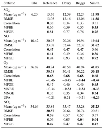
con-Table 1. Hourly statistics for the reference simulation with Po-lair3D (“Reference”), and plume-in-grid simulations, for three Gaussian parameterizations (“Sim.th.” stands for similarity theory). The simulation period is 2001-04-01–2001-09-27. The best statis-tics are highlighted in bold.
Statistic Obs Reference Doury Briggs Sim.th.
SO2
Mean (µg m−3) 6.20 13.76 12.59 12.24 11.98
RMSE 13.08 12.16 12.06 11.88
Correlation 0.35 0.34 0.33 0.31
MFBE 0.66 0.59 0.55 0.55
MFGE 0.81 0.77 0.76 0.75
NO
Mean (µg m−3) 10.42 20.93 20.26 19.94 19.64
RMSE 33.08 32.44 32.37 31.62
Correlation 0.47 0.47 0.47 0.46
MFBE 0.41 0.39 0.36 0.36
MFGE 0.94 0.93 0.92 0.92
O3
Mean (µg m−3) 56.87 40.24 40.58 40.94 41.05
RMSE 30.58 30.41 30.22 30.18
Correlation 0.68 0.68 0.68 0.68
MFBE −0.46 −0.45 −0.44 −0.44
MFGE 0.47 0.46 0.46 0.45
MNBE −0.34 −0.33 −0.33 −0.33
MNGE 0.35 0.35 0.34 0.34
UPA −0.21 -0.21 −0.21 −0.20
NO2
Mean (µg m−3) 34.64 35.84 35.47 35.28 35.23
RMSE 20.57 20.64 20.74 20.81
Correlation 0.58 0.57 0.57 0.57
MFBE 0.06 0.05 0.04 0.04
MFGE 0.47 0.47 0.47 0.47
sidering (1) the relatively small contribution of point sources in the total emissions, and (2) that statistics are computed on background stations, which are not located in the vicinity of major point sources. However, there is a clear improve-ment for NO and SO2. The RMSE is reduced by 9% in the case of SO2 and 4.5% for NO. On the contrary, the re-sults for NO2and O3are globally unchanged. This tends to show that the use of a subgrid-scale treatment of emissions has more impact on the primary pollutants than on secondary species. Moreover, the point sources account for a large part of SO2emissions, whereas NOxand O3depend more on traf-fic emissions. Also, since SO2is not a very reactive species, the plume-in-grid impact can be carried further downwind than for very reactive species (see Sect. 4.2).
4.1.3 Results on stations
5 10 15 20
RMSE
-10.3% -15.0% -6.2%
-8.1%
-12.5% -11.8% -8.9% -13.1% -16.2% -9.4%
-11.6%
6.2%
-8.4%
-17.4%
-13.6%
-14.2%
-0.8% -12.2%
-10.7%
(a) SO2
10 20 30 40 50
RMSE
-4.2%
-3.3% -5.9% -4.4%
-4.1%
-6.9% -3.6% -4.9% -2.8% -4.6% -4.5%
-4.5% -4.1% -3.2% -5.0% -5.2%
-1.3%
-6.1%
-6.7%
-3.0%
-2.2%
-0.3% -5.0%
(b) NO
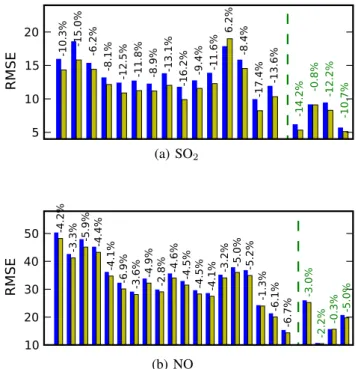
Fig. 5. RMSE (µg m−3) at stations for the whole period (April– September), for reference model (blue, first bar) and plume-in-grid model with similarity theory (yellow, second bar). The difference between the plume-in-grid and reference RMSE is indicated above the bars for each station, in percent. The first group of bars is for urban stations (percent indicated in black), the second group is for periurban and rural stations (percent in green).
Here, the parameterization used for the plume-in-grid con-figuration is similarity theory. Similarly good results (not shown here) were also found with the Briggs parameteriza-tion. The RMSE decrease ranges from 6.2% to 17.4% for SO2, and from 1.3% to 6.9% for NO, at urban stations. The results for periurban and rural stations are shown separately from the urban results. These stations are less influenced by traffic emissions, so the impact of point sources may be higher. However, they are farther from the sources than the urban stations. The overall RMSE on six months does show a significant impact at these stations, but no higher than the urban values. However, on particular days when the wind direction is such that one of these stations is downwind of the neighboring sources, the plume-in-grid impact is much higher (Sect. 4.2.2).
The results for NO2and O3are not shown, since the im-pact at particular stations was smaller, and well distributed among the stations: the RMSE for O3decreases by 0.2% to 2%, while the RMSE for NO2increases by about the same amount.
4.2 Spatial variability
In this section, we assess how the impact of a subgrid treat-ment of emissions is spatially distributed. The plume-in-grid
1.5 2.0 2.5 3.0 3.5 48.2
48.4 48.6 48.8 49.0 49.2
3.0 6.0 9.0 12.0 15.0 18.0 21.0 24.0 27.0
(a) SO2– Reference
1.5 2.0 2.5 3.0 3.5 48.2
48.4 48.6 48.8 49.0 49.2
3.0 6.0 9.0 12.0 15.0 18.0 21.0 24.0 27.0
(b) SO2– Plume-in-grid
1.5 2.0 2.5 3.0 3.5 48.2
48.4 48.6 48.8 49.0 49.2
0.0 1.5 3.0 4.5 6.0 7.5 9.0 10.5
(c) SO2– Reference - background
1.5 2.0 2.5 3.0 3.5 48.2
48.4 48.6 48.8 49.0 49.2
0.0 1.5 3.0 4.5 6.0 7.5 9.0 10.5
(d) SO2– Reference - plume-in-grid
Fig. 6.SO2concentrations over Paris region averaged over the
sim-ulation period, at ground level.(a)and(b)show the concentrations for the reference and the plume-in-grid simulation, respectively, in µg m−3. (c)shows the differences between mean ground concen-trations with and without point sources for the reference simulation.
(d)shows the differences between mean ground concentrations with and without plume-in-grid treatment.
simulation used henceforth is the similarity-theory simula-tion, which gave the best results in Sect. 4.1.
4.2.1 Impact on averaged concentrations
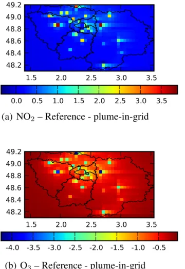
1.5 2.0 2.5 3.0 3.5 48.2
48.4 48.6 48.8 49.0 49.2
0.0 0.5 1.0 1.5 2.0 2.5 3.0 3.5
(a) NO
2– Reference - plume-in-grid
1.5 2.0 2.5 3.0 3.5
48.2 48.4 48.6 48.8 49.0 49.2
-4.0 -3.5 -3.0 -2.5 -2.0 -1.5 -1.0 -0.5
(b) O
3– Reference - plume-in-grid
Fig. 7.NO2and O3concentrations over Paris region averaged over
the simulation period, at ground level, in µg m−3. (a)shows the differences between mean ground concentrations with and without subgrid treatment for NO2.(b)shows the differences between mean
ground concentrations with and without plume-in-grid treatment for O3.
localized around the sources locations, since there is less hor-izontal diffusion.
Figure 6a shows two main SO2emission locations (except the urban area, at the center of the domain): at the north-west and south-east parts of the simulation domain. The north-western location is not due to point sources (there are no differences in that area when excluding point sources of the simulation – see Fig. 6c). The point source with the high-est emission rate is located in the south-east part of the do-main (see Fig. 3), which is also clearly shown by Fig. 6c. This is also where the use of the plume-in-grid model has the most impact, as shown in Fig. 6d. Here, the source height is about 80 m, so the plume stays higher with the plume-in-grid model, inducing lower ground concentrations.
The use of plume-in-grid also tends to lower the ground concentrations of NO and NO2 at point sources locations.
Figure 7 shows the results for NO2 and O3concentrations. The ground concentrations of O3are higher with the plume-in-grid treatment. This comes from the titration of back-ground O3by the NO emissions from point sources. Since the plume-in-grid treatment for NOx sources infers lower NOxconcentrations, it also results in slightly higher concen-trations of O3at ground level (there is less titration). 4.2.2 Results for particular days
We now analyze the particular case of a few specific days, in order to infer whether the impact of a subgrid-scale treatment for emissions depends on the meteorological situation. The first variable or influence is, of course, the wind direction: stations may locally significantly be impacted when situated downwind of sources. Moreover, the plume-in-grid impact may be more important during low-dispersion cases, when the Eulerian model significantly over-estimates the horizon-tal plume dilution. For primary pollutants, we selected two consecutive days, when the wind direction was such that several stations were downwind of the main sources: 23 and 24 August 2001. During these days, the wind speed ranged from 0.4 m s−1to 2.6 m s−1, and the averaged bound-ary layer height was 600 m. Those are typical values for low-dispersion days when concentrations of primary pollutants are higher than usual.
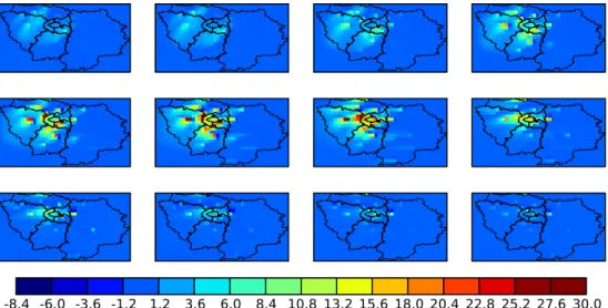
Figure 8 shows the evolution of the difference between reference and plume-in-grid ground concentrations for SO2, during twelve hours on 23 August. The maps show the hourly concentrations, from 03:00 (local hour) to 14:00 the same day. During these hours, the wind direction turns, and the wind speed decreases. In the first seven maps, the south-east source plume is clearly seen, and the plume-in-grid ef-fect on this plume is to lower the concentrations (the dif-ferences are positive). The plume direction is south-south-west and clearly impacts some stations (especially the sta-tion “MELUN”; stasta-tions23 on the Fig. 3). Another plume is visible in these first figures, located in the center-south of the domain. In this plume also, the plume-in-grid concen-trations are much lower than the reference concenconcen-trations. In the last five maps, the situation is very stable, with a very low wind speed (around 0.5 m s−1), and concentrations are very high. In the plume-in-grid model, the puffs do not travel very far from the source before being transferred into the Eulerian model (600 m for an injection time of 20 min). The concen-trations simulated by the plume-in-grid model are particu-larly high during such low-dispersion episodes, since there is no artificial dilution as in the Eulerian model. When the puffs are transferred in the Eulerian model and touch the ground, downwind of the sources, it thus induces higher ground con-centrations (differences are negative).
-20.1-17.6-15.1-12.6-10.1-7.6 -5.1 -2.6 -0.1 2.4 4.9 7.5 10.0 12.5 15.0 17.5 20.0 22.5 25.0
Fig. 8.Evolution of the difference between reference and plume-in-grid SO2ground concentrations during twelve hours, from 23 August at
03:00 (local hour) to 23 August at 14:00. Unit is µg m−3. Plume-in-grid concentrations are subtracted to the reference concentrations.
0 10 20 30 40 50 0
5 10 15 20 25 30
Reference Plume-in-grid Observations
(a)MELUN
0 10 20 30 40 50 0
10 20 30 40 50
Reference Plume-in-grid Observations
(b)VITRY-SUR-SEINE
0 5 10 15 20 25 30 35 40 45 0
10 20 30 40 50 60
Reference Plume-in-grid Observations
(c)IVRY-SUR-SEINE
0 10 20 30 40 50 0
10 20 30 40 50 60
Reference Plume-in-grid Observations
(d)PARIS12eme
0 10 20 30 40 50 0
10 20 30 40 50
Reference Plume-in-grid Observations
(e)AUBERVILLIERS
0 5 10 15 20 25 30 35 40 0
10 20 30 40 50 60 70
Reference Plume-in-grid Observations
(f)LADEFENSE
Fig. 9. SO2 profiles during two days, from 2001-08-23 at 03:00
(local time) to 2001-08-25 at the same hour, at six stations. Profiles are shown for the measurement, reference simulation and plume-in-grid simulation with similarity theory.
is impacted by the south-east plume at the beginning of the period. In the remaining period, the measured concentra-tions are globally low. The plume-in-grid treatment induces less over-estimation of the plume impact, but does not mod-ify the arrival time: even though the plume-in-grid treat-ment delays the plume arrival, it is negligible on hourly-averaged concentrations. The next three stations, VITRY-SUR-SEINE, IVRY-SUR-SEINE and PARIS12eme are situ-ated in the southern part of Paris (which is in the middle of the simulation domain), within the second plume observed in Fig. 8. Here, the plume-in-grid profiles are much closer to the observations than the reference values. Finally, two stations situated in the northern part of Paris are also shown, since they are upwind of the main sources: the plume-in-grid impact is much lower at these stations, but still beneficial to the performance. The observed concentrations of SO2 are much lower than the simulated values. Since only the mean emission rate over the year is available for all sources, they are assumed to be continuously emitting, and the same tem-poral profile is applied to all of them. This is an approxima-tion, since some of the main point sources are thermal power plants, which are only emitting during some periods. This leads to uncertainties and over-estimation of the emissions during some days, especially in summertime when many of these power plants are shut down.
-8.4 -6.0 -3.6 -1.2 1.2 3.6 6.0 8.4 10.8 13.2 15.6 18.0 20.4 22.8 25.2 27.6 30.0
Fig. 10.Evolution of the difference between reference and plume-in-grid NO ground concentrations during twelve hours, from 23 August at 03:00 (local hour) to 23 August at 14:00. Unit is µg m−3. Plume-in-grid concentrations are subtracted to the reference concentrations.
-12.9-12.0-11.1-10.1 -9.2 -8.2 -7.3 -6.4 -5.4 -4.5 -3.5 -2.6 -1.6 -0.7 0.2 1.2 2.1 3.1 4.0
Fig. 11.Evolution of the difference between reference and plume-in-grid O3ground concentrations during twelve hours, from 20 August at
03:00 (local hour) to 20 August at 14:00. Unit is µg m−3. Plume-in-grid concentrations are subtracted to the reference concentrations.
concentrations, since NO emissions are mainly due to traffic. Thus, no significant differences are observed on the stations profiles (not shown). It should also be noticed that for NO as well as for SO2, the differences are larger during the morn-ing (second row of maps on Figs. 8 and 10). Durmorn-ing this period, concentrations are higher, since emissions are high and the boundary layer is not fully developed yet, leading to less vertical mixing than during the rest of the day. This is not specific to these particular days.
To study O3, the selected day is the 20 August. It is a day of low to medium dispersion, with a wind speed between 1 and 2 m s−1. This date is retained because the plume-in-grid impact is widely spread, and differences in ozone concen-trations are transported over large distances. The effect of
1.5 2.0 2.5 3.0 3.5 48.2
48.4 48.6 48.8 49.0 49.2
0.00 0.00 0.01 0.01 0.01 0.01 0.02 0.02 0.02 0.03
Fig. 12. Mean differences betweenKz values at 50 m with and
without the minimum urban value ofKzmin= 0.5 m2s−1. Diffusion
coefficients are averaged over six months.
are less localized than the differences on the primary pollu-tants. This impact is not seen on the measurement stations, since they are all located within the urban area – at the center of the domain – whereas the O3impact occurs mostly down-wind of the urban plume, in rural areas.
5 Sensitivity analysis
5.1 Influence of vertical diffusion 5.1.1 Urban vertical diffusion
As explained in Sect. 3.1, when computingKz fields with
the Troen-Mahrt parameterization, a minimum value is used in order to ensure a minimum vertical diffusion everywhere. In rural areas, it is set toKzmin=0.2 m2s−1. In urban areas, however, the vertical diffusion is increased, due to the tur-bulence induced by heat and the particular radiative property of the urban canopy. Thus, the minimum value is increased for these areas, and set toKzmin=0.5 m2s−1. This value is mostly activated during nighttime and very stable situations. Figure 12 shows the mean differences over six months, be-tween vertical coefficient values at 50 m, with and without the minimum urban value ofKzmin=0.5 m2s−1. In this sec-tion, the impact of such a change on the simulation results is assessed.
The results are shown for three simulations: (1) a simu-lation with the Eulerian model, andKzmin=0.2 m2s−1 ev-erywhere (labeled “Kz”), (2) a simulation with the
Eule-rian model, andKzmin=0.5 m2s−1over urban areas (labeled “Kzurban”) and (3) simulation with the plume-in-grid
treat-ment for point sources, andKzmin=0.5 m2s−1 over urban areas (labeled “plume-in-grid”). The simulations (2) and (3) are the reference simulation and the plume-in-grid simula-tion with similarity theory, respectively – they are the same as those already analyzed in Sect. 4. Table 2 shows the same statistical metrics as Table 1, for all species and for six months (1 April 2001–27 September 2001). Increasing the
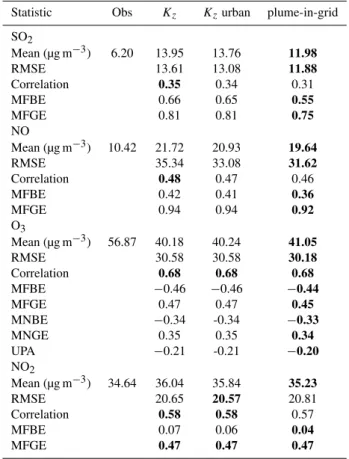
Table 2. Hourly statistics: comparison between (1) the simulation with the Eulerian model and a uniform minimal value forKzmin, (2)
the reference simulation, that is, the Eulerian model with a specific value forKzminin urban areas, and (3) the plume-in-grid results
with similarity theory. The simulation period is 2001-04-01–2001-09-27. The best statistics are highlighted in bold.
Statistic Obs Kz Kzurban plume-in-grid
SO2
Mean (µg m−3) 6.20 13.95 13.76 11.98
RMSE 13.61 13.08 11.88
Correlation 0.35 0.34 0.31
MFBE 0.66 0.65 0.55
MFGE 0.81 0.81 0.75
NO
Mean (µg m−3) 10.42 21.72 20.93 19.64
RMSE 35.34 33.08 31.62
Correlation 0.48 0.47 0.46
MFBE 0.42 0.41 0.36
MFGE 0.94 0.94 0.92
O3
Mean (µg m−3) 56.87 40.18 40.24 41.05
RMSE 30.58 30.58 30.18
Correlation 0.68 0.68 0.68
MFBE −0.46 −0.46 −0.44
MFGE 0.47 0.47 0.45
MNBE −0.34 -0.34 −0.33
MNGE 0.35 0.35 0.34
UPA −0.21 -0.21 −0.20
NO2
Mean (µg m−3) 34.64 36.04 35.84 35.23
RMSE 20.65 20.57 20.81
Correlation 0.58 0.58 0.57
MFBE 0.07 0.06 0.04
MFGE 0.47 0.47 0.47
vertical diffusion in urban areas improves the overall statis-tics by reducing the over-estimation of emitted species. As in the case of plume-in-grid, the secondary pollutants, espe-cially O3, are less sensitive to the model configuration than the primary pollutants, since vertical gradients are smaller. The most impacted species is NO, which can be explained by the strong vertical concentration gradient for this species, with higher concentration at ground level due to traffic emis-sions. Thus, increasing the vertical diffusion tends to lower NO ground concentrations.
5.1.2 Eulerian and Gaussian vertical diffusion
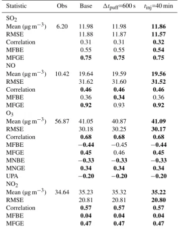
Table 3. Hourly statistics: comparison between (1) Base simulation: plume-in-grid with similarity theory, tinj=20 min
and 1tpuff=100 s, (2) plume-in-grid with similarity theory and 1tpuff=600 s, (3) plume-in-grid with similarity theory and tinj=40 min. The simulation period is 2001-04-01–2001-09-27. The
best statistics are highlighted in bold.
Statistic Obs Base 1tpuff=600 s tinj=40 min
SO2
Mean (µg m−3) 6.20 11.98 11.98 11.86
RMSE 11.88 11.87 11.57
Correlation 0.31 0.31 0.32
MFBE 0.55 0.55 0.54
MFGE 0.75 0.75 0.75
NO
Mean (µg m−3) 10.42 19.64 19.59 19.56
RMSE 31.62 31.60 31.52
Correlation 0.46 0.46 0.46
MFBE 0.36 0.34 0.36
MFGE 0.92 0.93 0.92
O3
Mean (µg m−3) 56.87 41.05 40.87 41.09
RMSE 30.18 30.25 30.17
Correlation 0.68 0.68 0.68
MFBE −0.44 −0.45 −0.44
MFGE 0.45 0.46 0.45
MNBE −0.33 −0.33 −0.33
MNGE 0.34 0.34 0.34
UPA −0.20 −0.20 −0.20
NO2
Mean (µg m−3) 34.64 35.23 35.32 35.22
RMSE 20.81 20.81 20.80
Correlation 0.57 0.57 0.57
MFBE 0.04 0.04 0.04
MFGE 0.47 0.47 0.47
for Gaussian standard deviations gives better results than Briggs’ or Doury’s formulas, although the estimates of ver-tical diffusion given by the last two formulas are generally higher. In particular, when more than a quarter of the cell is urban, Briggs’ formulas are automatically switched from rural to urban formulas, which give a much larger vertical diffusion. However, overall results with Briggs formulas are not quite as good as with similarity-theory parameterization. This may be due to a compensating effect between rural and urban plumes that impact a given station, depending on a meteorological situation. Besides, most of the point sources treated by the plume-in-grid model in this study are elevated sources (second or third vertical level). Thus, the main effect of the plume-in-grid treatment is to hold the plume aloft for a longer time period, and the enhanced vertical diffusion is not as important as for near-ground sources.
5.2 Influence of local-scale modeling
The “local scale” refers to the characteristic scale where the subgrid modeling of sources occur. It is the near-source area where the Gaussian puff model is used, and it is determined by the choice of the injection criterion (Sect. 2.2). The im-pact of the standard deviation parameterizations has already been addressed. In this section, the sensitivity to two other parameters is analyzed: the injection timetinj and the time step between two puffs1tpuff. Hereafter, the “base” simu-lation refers to the plume-in-grid simusimu-lation with similarity theory used in the previous parts of the study. For that base case,tinj=20 min and1tpuff=100 s.
Table 3 gives the global statistics for the base simulation (already shown), as well as for the simulations with (1) a larger time step between two puffs (1tpuff=600 s) and (2) a larger injection time (tinj=40 min). Increasing the time step between two puffs does not significantly change the results. SO2is fairly insensitive to that parameter. The results for the reactive species are slightly different from the base results: worse for O3and NO2, and better for NO. The time step be-tween two puffs is important for reactive species, since it de-termines the overlap volume between two consecutive puffs. If this time step is not sufficient, the overlap volume between two consecutive puffs is small during the first time steps. On the other hand, each puff contains a larger amount of quan-tity: the quantity for each puff is given byQ=Qs×1tpuff, whereQs is the source rate in mass unit per second, for a
given species. As a result, the chemistry within each puff is enhanced. In the case of NOxand O3chemistry, this leads to slightly more titration, which means a decrease in NO and O3 concentrations, and an increase of NO2concentrations. The impact of this phenomenon is not very large, but not negli-gible compared to the global plume-in-grid impact for these species.
The injection time has much more influence on SO2than on the reactive species. Using the Gaussian puff model for a longer time allows to widen the scope of the plume-in-grid impact, thus improving the results for SO2. Compared to the base case (plume-in-grid withtinj=20 min), the RMSE on urban stations are improved by 0.4% to 8%, with an im-provement at most stations around 2%. This is an additional improvement, compared to the initial difference brought by the base case (in Fig. 5). The impact on NO results, however, is not so large: the global statistics are not significantly mod-ified, and the highest improvement on stations is 0.8%. The results for NO2and O3are still less impacted. Thus, for reac-tive species, increasing the injection time is not a major im-provement: after some time, the plume composition becomes closer to the background composition, and the plume-in-grid treatment induces less additional differences.
base briggs
dtpuff=600stinj=40mins 0.0
0.2 0.4 0.6 0.8 1.01.2 1.4 1.6
RMSE difference
(a) SO2
base briggs
dtpuff=600stinj=40mins 0.0
0.10.2 0.3 0.4 0.5 0.6 0.7 0.8
RMSE difference
(b) NOx
base briggs
dtpuff=600stinj=40mins 0.00
0.05 0.10 0.15 0.20 0.25 0.30 0.35 0.40 0.45
RMSE difference
(c) O3
Fig. 13.Differences (Polair3D - plume-in-grid) in RMSE (µg m−3), computed on all stations and six months for SO2, NOx and O3.
(1) “base”: plume-in-grid with similarity theory,tinj=20 minutes and1tpuff=100 s, (2) “briggs”: base case with Briggs formulas
instead of similarity theory, (3) base case with1tpuff=600s, (4)
base case withtinj=40 minutes. Dotted line : base results. Green
bars correspond to the highest sensitivity for each species.
is sensitive to the injection time, NOx to the diffusion pa-rameterization, and O3is mostly impacted by the time step between two puffs. This illustrates the importance of care-fully choosing all these parameters, depending on the target species and the computational time.
6 Conclusions
The plume-in-grid model implemented on the Polyphemus platform has been applied to regional photochemistry over Paris region. Model-to-data comparisons have been per-formed and compared to the results obtained when using the Eulerian model Polair3D alone. The plume-in-grid impact on the mean results for six months is not large, although sig-nificant for primary emitted species. This impact is higher when using the similarity-theory parameterization for stan-dard deviations, which performs better than the other two pa-rameterizations. With that scheme, the RMSEs at the stations are reduced by up to 17% in the case of SO2and up to 7% for NO. The impact on NO2 and O3is much smaller, since they are more influenced by traffic emissions than by point sources.
Using a plume-in-grid treatment for point emissions has a significant impact on the near-source concentrations. It may be carried up to some distance downwind, depending on the meteorological situation. Low-dispersion situations, when the Eulerian model significantly over-estimates the
horizon-tal plume dilution, also increase the plume-in-grid benefit. This can be observed on the station profiles for particular days, when some measurement stations are located down-wind of the main sources.
The effect of the plume-in-grid model is to lower the ground concentrations of emitted species, through two mech-anisms: (1) the plume is held aloft longer than in the Eulerian model, and (2) the near-source vertical diffusion and chem-istry are better represented. It results in higher O3 ground concentrations, since there is less titration. Further down-wind, when the plume touches the ground, the reverse may be observed, as the titrated O3 plume is transported to the ground.
When addressing the sensitivity to the urban vertical dif-fusion, which is often under-estimated, the primary pollu-tants are again the most impacted species. The influence of two plume-in-grid parameters was also assessed. The time step between two puff emissions mostly influences the chemically reactive species – near-source chemical rates are slightly over-estimated when the time step is too large. On the contrary, the almost-passive species SO2 is mostly im-pacted by a change in the injection time. Since these two parameters determine the number of puffs handled by the model and the corresponding computational time, they must be carefully chosen according to the target species.
Future developments and applications of this model in-clude an application at continental scale over Europe, and an extension to handle aerosol chemistry. In addition, the model will be extended to the modeling of line sources in order to use the subgrid-scale treatment with road emissions. This application is expected to show much more striking results, because of the importance of traffic emissions on the pollu-tants of interest. Another important point would be to include simplified in-plume chemistry, as described in Karamchan-dani et al. (1998), in order to significantly reduce the com-putational time for puffs chemistry. This would be particu-larly interesting since the plume-in-grid impact on secondary species is not very large.
Appendix A Overlapping puffs
We consider that two puffsαandβ overlap if the distance between their centers is smaller than 2
σjα+σjβ
in one di-rectionj∈(x,y,z). We notehcαAithe integral over space of the concentration of speciesAin the puffα. The quantity of speciesAin puffαis thusQαA= hcαAi. We define the puff volume as
Vα=
hcAαi2
hcAα2i. (A1)
of Gaussian puffs, the “real” volume is infinite. This defini-tion is verified in the case of puffs with a finite volume and a uniform concentration. Here,cαa is the product of gaussian shapes in the three directions, so the puff’s volume can be computed as a function of the gaussian standard deviations
Vα=23π3/2σxασ α yσ
α
z. (A2)
The overlap volume between two puffsαandβ is noted
Vαβand defined as Vαβ
VαVβ
= hc
α Ac
β Ai
hcαAihcAβi
. (A3)
Therefore, the quantity of speciesA transported by the puffαisQαA=Vα×cAα, and the quantity of speciesAwithin
the volume of puffα, but coming from any overlapping puff
β isQαβA =Vαβ×cβA. Hence, we define the overlap
concen-tration of species A and puff α as the total quantity of A
from all the overlapping puffs, diluted within the volumeVα
(Eq. A4):
b
cAα=X
β
QβA Vαβ VαVβ
=X
β
cβA Vαβ Vα
(A4)
The chemistry during a time step1tis computed with the overlap concentrations from all puffs. The overlap concen-tration at the end of the time step is then
b
cAα(t+1t )=cbAα(t )+1cbαA. (A5)
However, the species produced within the overlap volumes are taken twice into account: once with the overlapping con-centrations of puff α, and once with those of puffβ. The production (or loss) must be distributed into the two puffs to ensure the mass conservation. One option (Karamchandani et al., 2000) is to take
1QαA=1cbαA×Q
α A(t ) b
cAα(t ) (A6)
as the actual quantity of speciesAcreated during1tin puff
α.
Acknowledgements. We thank Christian Seigneur for his help in the development of the puffs chemistry. We also thank Airparif for having provided the emission inventory and the observations, and Marilyne Tombette for providing the programs processing Airparif emissions.
Edited by: S. Galmarini
References
Boutahar, J., Lacour, S., Mallet, V., Qu´elo, D., Roustan, Y., and Sportisse, B.: Development and validation of a fully modular platform for numerical modelling of air pollution: POLAIR, Int. J. Env. Pollut., 22, 17–28, 2004.
Brandt, J.: Modelling Transport, Dispersion and Deposition of Pas-sive Tracers from Accidental Releases, Ph.D. thesis, National Environmental Research Institute, 1998.
Chang, J. and Hanna, S.: Air quality model performance evaluation, Meteorol. Atmos. Phys., 87, 167–196, 2004.
EPA: Guideline for regulatory application of the urban airshed model, Tech. Rep. EPA-450/4-91-013, US EPA, 1991.
EPA: Guidance on the use of models and other analyses in attain-ment demonstrations for the 8-hr ozone NAAQS, Tech. Rep. EPA-450/R-99-004, US EPA, 2005.
Gillani, N.: Ozone formation in pollutant plumes: Development and application of a reactive plume model with arbitrary crosswind resolution, Tech. Rep. EPA-600/S3-86-051, US Environmental Protection Agency, Research Triangle Park, NC, USA, 1986. Godowitch, J.: Simulations of aerosols and photochemical species
with the CMAQ plume-in-grid modeling system, 3rd CMAS Models-3 Users’ Conference, Univ. North Carolina, Chapel Hill, NC, USA, 2004.
Hanna, S. and Paine, R.: Hybrid Plume Dispersion Model (HPDM) Development and Evaluation, J. Appl. Meteor., 28, 206–224, 1989.
Karamchandani, P., Koo, A., and Seigneur, C.: Reduced gas-phase kinetics mechanism for atmospheric plume chemistry, Environ. Sci. Technol., 32, 1709–1720, 1998.
Karamchandani, P., Santos, L., Sykes, I., Zhang, Y., Tonne, C., and Seigneur, C.: Development and evaluation of a state-of-the-science reactive plume model, Environ. Sci. Technol., 34, 870– 880, 2000.
Karamchandani, P., Seigneur, C., Vijayaraghavan, K., and Wu, S.: Development and application of a state-of-the-science plume-in-grid model, J. Geophys. Res., 107(D19), 4403, doi:10.1029/ 2002JD002123, 2002.
Korsakissok, I. and Mallet, V.: Comparative study of Gaussian dis-persion formulas within the Polyphemus platform: evaluation with Prairie Grass and Kincaid experiments, J. Appl. Meteor., 48, 2459–2473, doi:10.1175/2009JAMC2160.1, 2009.
Korsakissok, I. and Mallet, V.: Subgrid-scale treatment for major point sources in an Eulerian model: a sensitivity study on the ETEX and Chernobyl cases, J. Geophys. Res., 115, D03303, doi: 10.1029/2009JD012734, 2010.
Kumar, N. and Russell, A.: Development of a computationally ef-ficient, reactive subgrid-scale plume model and the impact in the northern United States using increasing levels of chemical de-tails, J. Geophys. Res., 101, 16737–16744, 1996.
Louis, J.-F.: A parametric model of vertical eddy fluxes in the at-mosphere, Bound.-Layer Meteor., 17, 187–202, 1979.
Mallet, V., Qu´elo, D., Sportisse, B., Ahmed de Biasi, M., Debry, ´
E., Korsakissok, I., Wu, L., Roustan, Y., Sartelet, K., Tombette, M., and Foudhil, H.: Technical Note: The air quality modeling system Polyphemus, Atmos. Chem. Phys., 7, 5479–5487, 2007, http://www.atmos-chem-phys.net/7/5479/2007/.
Morris, R., Yocke, M., Myers, T., and Kessler, R.: Development and testing of UAM-V: A nested-grid version of the Urban Airshed Model, in: Proceedings of the AWMA conference: Tropospheric ozone and the environment II, Pittsburgh, PA, USA, 1991. Seigneur, C., Tesche, T., Roth, P., and Liu, M.: On the treatment
of point source emissions in urban air quality modeling, Atmos. Environ., 17, 1655–1676, 1983.
Stockwell, W. R., Kirchner, F., Kuhn, M., and Seefeld, S.: A new mechanism for regional atmospheric chemistry modeling, J. Geophys. Res., 102, 25847–25879, 1997.
Taylor, G.: Diffusion by continuous movements, Proc. Lnd. Math. Soc., 20, 196–211, 1921.
Tombette, M. and Sportisse, B.: Aerosol modeling at a regional scale: Model-to-data comparison and sensitivity analysis over Greater Paris, Atmos. Environ., 41, 6941–6950, 2007.
Troen, I. and Mahrt, L.: A simple model of the atmospheric bound-ary layer; sensitivity to surface evaporation, Bound.-Layer Me-teor., 37, 129–148, 1986.