S. R. Freitas1, K. M. Longo2, J. Trentmann3,*, and D. Latham4
1Center for Weather Forecasting and Climate Studies, INPE, Cachoeira Paulista, Brazil 2Center for Space and Atmospheric Sciences, INPE, S˜ao Jos´e dos Campos, Brazil 3University of Mainz, Mainz, Germany
4USDA Forest Service, Montana, USA
*now at: German Weather Service, Offenbach, Germany
Received: 29 May 2009 – Published in Atmos. Chem. Phys. Discuss.: 7 July 2009 Revised: 16 December 2009 – Accepted: 11 January 2010 – Published: 21 January 2010
Abstract.Vegetation fires emit hot gases and particles which are rapidly transported upward by the positive buoyancy gen-erated by the combustion process. In general, the final ver-tical height that the smoke plumes reach is controlled by the thermodynamic stability of the atmospheric environment and the surface heat flux released by the fire. However, the presence of a strong horizontal wind can enhance the lat-eral entrainment and induce additional drag, particularly for small fires, impacting the smoke injection height. In this paper, we revisit the parameterization of the vertical trans-port of hot gases and particles emitted from vegetation fires, described in Freitas et al. (2007), to include the effects of environmental wind on transport and dilution of the smoke plume at its scale. This process is quantitatively represented by introducing an additional entrainment term to account for organized inflow of a mass of cooler and drier ambient air into the plume and its drag by momentum transfer. An extended set of equations including the horizontal motion of the plume and the additional increase of the plume ra-dius is solved to simulate the time evolution of the plume rise and the smoke injection height. One-dimensional (1-D) model results are presented for two deforestation fires in the Amazon basin with sizes of 10 and 50 ha under calm and windy atmospheric environments. The results are compared to corresponding simulations generated by the complex non-hydrostatic three-dimensional (3-D) Active Tracer High res-olution Atmospheric Model (ATHAM). We show that the
1-Correspondence to:S. R. Freitas ([email protected])
D model results compare well with the full 3-D simulations. The 1-D model may thus be used in field situations where extensive computing facilities are not available, especially under conditions for which several optional cases must be studied.
1 Introduction
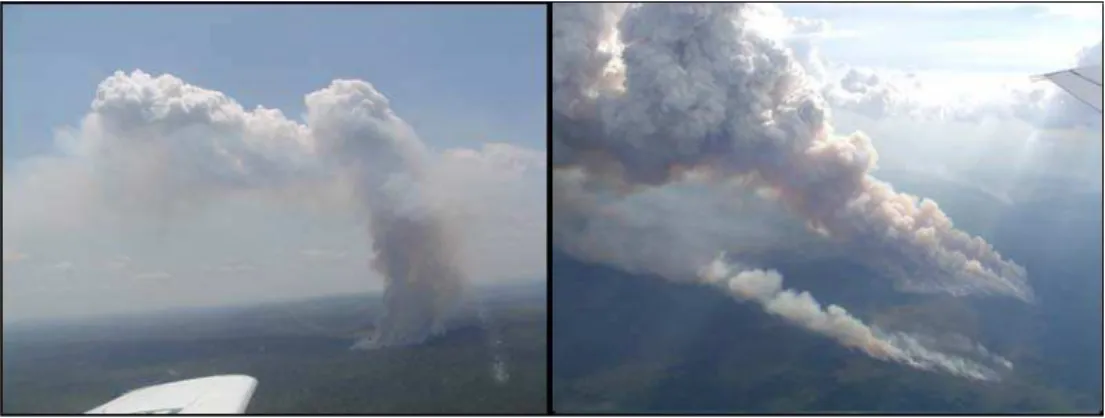
Fig. 1. Photographs of the smoke plume rise produced from two deforestation fires in the Amazon basin under calm (left) and windy (right) environments. Both photos were taken from aircraft. Note that size of the fires and the plume height differs substantially between the plumes. (Pictures taken by M. O. Andreae and M. Welling).
different deforestation fires in the Amazon basin (Fig. 1). The plume shown on the left moves upward with only a slight deviation from the vertical, indicating plume development in a calm environment. However, the plume on the right shows much stronger deflection from the vertical, an indication of a windy environment. Note that both plumes are capped by cumulus, indicating that cloud microphysics might have had a significant role in the plume development. The ef-fect of ambient wind on the plume rise from volcanic sources has been studied by several authors. Graf et al. (1999) per-formed a set of sensitivity studies using a two-dimensional version of the Active Tracer High resolution Atmospheric Model (described here in Sect. 3.1) as a non-hydrostatic vol-cano plume model with explicit treatment of turbulence and microphysics. The authors applied this modeling system to simulate the impacts of environmental conditions on the ver-tical plume development. They found that, in general, a horizontal wind reduces the height reached by the plume. All environmental impacts were found to strongly depend on the intensity of the entrainment and, thus, on the quality of the calculated turbulence properties. Bursik (2001) ap-plied a 1-D theoretical model of a plume to study the inter-action between a volcanic plume and an ambient wind. He also shows that the enhanced entrainment from the wind de-creases the plume rise height, mainly at altitudes with the high wind speeds of the polar jet. To the author’s knowledge, no study on the impact of horizontal wind on the injection height of volcanic eruptions or wild fires is available that em-ploys three-dimensional model simulations. However, obser-vational and theoretical studies of volcanic eruptions (Ernst et al., 1994; Rose et al., 2003) and fire plumes (Cunning-ham et al., 2005; Cunning(Cunning-ham and Linn, 2007) have shown the relevance of three-dimensional aspects for the dynamical evolution of such plumes. Hence, the results obtained from 1-D and 2-D simulations have to be interpreted with care. For the present work, ATHAM is used for 3-D simulations
(see Sect. 3.1). In this paper we describe the improvement of the 1-D parameterization of the vertical transport of hot gases and particles emitted from vegetation fires, described in Freitas et al. (2007, hereafter F2007), to include the ef-fects of environmental horizontal wind on transport and dilu-tion of the smoke plume at its scale. This process is quantita-tively represented by introducing an additional entrainment term to represent the organized inflow of the ambient air into the plume, as well as the drag on the plume by the external ambient wind. The extra entrainment enhances the in-plume mixing with the cooler and drier ambient air. The net effect on the dynamics is a reduction of the in-plume velocity in the vertical through momentum transfer to the entrained air mass; while horizontally, there is a strong acceleration in the nearby surface layer as well as in the layers with strong am-bient wind shear. An extended set of equations, including the horizontal motion of the plume and increase of the plume radius, is now solved to simulate the time evolution of the plume rise and determine the final injection height.
In the methodology proposed by Freitas et al. (2006, 2007), the 1-D plume model is embedded in each column of 3-D low resolution atmospheric chemistry-transport mod-els (the hosts) to provide interactively the smoke injection height, in which trace gases and aerosols, emitted during the flaming phase of the vegetation fires, are released and then transported and dispersed by the prevailing winds simulated by them.
∂t ∂z 1+γ ∂T
∂t +w ∂T
∂z = −w g
cp−(λentr+δentr)(T−Te)
+ ∂T ∂t µp (2) ∂rv ∂t +w
∂rv
∂z = −(λentr+δentr)(rv−rve)+
∂rv ∂t µp (3) ∂rc ∂t +w
∂rc
∂z = −(λentr+δentr)rc+
∂r c ∂t µp (4) ∂rice,rain
∂t +w
∂rice,rain
∂z = −(λentr+δentr)rice,rain
+ ∂rice,rain ∂t µp
+sedimice,rain (5)
∂u ∂t +w
∂u
∂z= −(λentr+δentr)(u−ue) (6)
∂R ∂t +w
∂R ∂z =(
3 5λentr+
1
2δentr)R (7)
Herew,T,rv,rc,rrain,riceare the vertical velocity, air
tem-perature, water vapor, cloud, rain and ice mixing ratios, re-spectively, and are associated with in-plume air parcels. The velocityurepresents the horizontal velocity of the center of mass of the plume at levelz. In Eq. (1)γ is 0.5 and was introduced to compensate for the neglect of non-hydrostatic pressure perturbations (Simpson and Wiggert, 1969),gis the acceleration due the gravity andB is the buoyancy term re-lated to the difference of temperature between the in-plume air parcel and its environment air and includes the downward drag of condensate water. In the equations above the indexe
stands for the environmental value, all other variables refer to the center of mass of the plume. The termλentris the lateral entrainment given by
λentr=2α
R |w| (8)
where all variables are as previously defined. The dynamic entrainment term is proportional to the difference between the magnitudes of the ambient atmosphere and plume hor-izontal velocities, because there is no dynamic entrainment when both masses are moving at the same speed. Also,δentr
is inversely proportional to the plume radius size meaning that the bigger the plume, the less sensitive it is to this en-trainment process. The derivation Eq. (9) is given in Ap-pendix A.
Equation (1) is the vertical equation of motion. The new term (−δentrw) expresses the loss rate of in-plume vertical velocity due to momentum transfer to the ambient air mass entrained into the plume (environmental vertical velocity is assumed negligible when compared to the in-plume vertical velocity). Equations (2)–(5) express the first law of thermo-dynamics and mass continuity equations for water phases in-cluding the dynamic entrainment process. This process is included using the traditional bulk formulation, being ex-pressed by the product of the entrainment rate and the dif-ference between in-plume and ambient atmosphere values. Indexµp denotes the tendencies from cloud microphysics (see F2007 for a discussion about the cloud microphysics and sedimentation terms of these equations).
Equation (6) is introduced to represent the gain of horizon-tal velocity of the plume due to drag by the ambient air flow. It is the horizontal equation of motion and we assume that at the timescale of the plume rise both entrainment terms are main forcings for the horizontal acceleration. The horizontal entrainment terms are responsible for the bent-over plumes as seen in Fig. 1. The lower boundary condition for the solu-tion (u) of this equation isu(z=0)=0. From Eq. (6), with no ambient wind (ue(z)=0), the plume will develop only
Fig. 2. Temperature (solid) and dew point temperature (dashed) profiles from a rawinsonde launched in Rondonia (11 S, 60 W) shown by a skewT−logpdiagram. Case(A)depicts the condition at 18:00 UTC on 20 September 2002, classified as the calm case. (B)is the windy case corresponding to 18:00 UTC on 27 September 2002. (C)Horizontal wind magnitude profiles of the calm (dashed) and windy (solid) cases obtained from the rawinsondes.
3 Case studies and 1-D PRM comparisons with the ATHAM model
In this section we provide an evaluation of the 1-D PRM model performance and sensitivity to the new formulation for simulating the smoke plume rise of Amazon basin de-forestation fires, under different environmental conditions. Due the lack of observational data, we performed a set of numerical experiments of hypothetical prescribed fires and used the comprehensive 3-D ATHAM model to compare the 1-D model results and findings.
3.1 Model descriptions and conditions of the simulations
The numerical experiments were done under two selected thermodynamical situations. Figure 2 shows the two cases obtained from rawinsondes launched in the burning season of 2002 in the Amazon basin over a forested site and close to deforestation areas. Figure 2a depicts a typical atmospheric condition in the Amazon basin and central part of South America during the burning season at 18:00 UTC, normally the peak time of the diurnal cycle of basin fires. A rawin-sonde, launched at 18:00 UTC on 20 September 2002, shows a strong thermal inversion around 800 hPa with a very dry layer above. Figure 2b shows the atmospheric condition one week later and in the same region, which is quite different.
There was a weaker thermal inversion around 870 hPa and a much moister layer above compared with the previous case. In addition, these two cases also present a significant dif-ference in the horizontal wind magnitude (Fig. 2c). For the first case, the mean magnitude is approximately 2 m s−1from the surface to 500 hPa while the latter has values of approx-imately 4 to 5 m s−1. Because of these characteristics, the cases are labeled as “calm” and “windy”, respectively. Note also that there is strong wind shear in the first 1500 m for both situations, from 2 to 4 m s−1and 2 to 6 m s−1for calm and windy cases, respectively. The comparison between the two cases is interesting due to the different roles that cloud microphysics and ambient wind processes play on the posi-tion of the smoke injecposi-tion layer.
The Active Tracer High resolution Atmospheric Model (Oberhuber et al., 1998) is a three-dimensional atmospheric plume model, which has been designed and employed for the simulation of strong convective events, e.g., volcanic erup-tions (e.g., Graf et al., 1999; Herzog et al., 2003; Textor et al., 2003) and vegetation fires (e.g., Trentmann et al., 2002, 2006; Luderer et al., 2006). ATHAM solves the Navier-Stokes equation for a gas-particle mixture, based on exter-nal forcing including the transport of active tracers. Cloud microphysical processes are simulated using a two-moment scheme that predicts the numbers and mass mixing ratios of four hydrometeor classes and water vapor (Textor et al., 2006). The aerosol-cloud interactions are not considered in the simulations presented here.
Fire emissions are represented in ATHAM by prescrib-ing emission fluxes into the lowest atmospheric model layer over specified fire grid boxes. In the present study, only fluxes of heat, moisture and aerosol particles are considered. The model simulations presented here were conducted on a stretched grid with a minimum horizontal and vertical model grid spacing of 50 m×50 m×50 m in the center and increas-ing grid spacincreas-ing towards the edges of the model domain. The total model domain covered 15 km×15 km×23 km cor-responding to 86×86×80 grid boxes. The maximum time step was set to 1.5 s, the minimum time step was determined dynamically by the Courant-Friedrich-Lewy (CFL) criterion. Evaluating the quality of ATHAM simulations with reality is a challenging task. The ATHAM model results substan-tially depend on the initial and boundary conditions of the atmosphere and the fire. While the atmospheric conditions are usually known within an acceptable accuracy, fire infor-mation (e.g., the amount of biomass burned within a known period of time) is rarely available. ATHAM results have been evaluated for two vegetation fires, for which some informa-tion on the fuel was available: the Quinault Fire at the US Pacific Coast and the Chisholm fire in Canada. In both cases, ATHAM was able to realistically simulate the evolution of the plume and its injection height (Trentmann et al., 2002, 2006).
The 1-D PRM was run using a constant grid space resolu-tion of 100 m with a top at 20 km height. The model time step
was dynamically calculated following the CFL stability cri-terion, not exceeding 5 s. The microphysics is resolved using time splitting (1/3 of dynamic time step). The upper bound-ary condition is defined as a Rayleigh friction layer with 60 s timescale. Typically, steady state is reached within 50 min, this number being the upper limit of the time integration. The final rise of the plume (the plume height top) is determined by the height for which the vertical velocity of the in-plume air parcel is less than 1 m s−1.
In total, we performed twelve simulations. Four of them were conducted using the ATHAM model, which was ini-tialized with the atmospheric conditions described above and fire sizes of 10 and 50 ha. For simulations which used the 1-D PRM configuration, we performed four additional simula-tions besides those with the same configuration as ATHAM. These four simulations did not account for the effect of en-vironmental horizontal wind drag. In these simulations, the horizontal ambient wind was set to zero (ue(z)=0). Table 1
summarizes the simulations.
3.2 Description and results of the ATHAM model runs
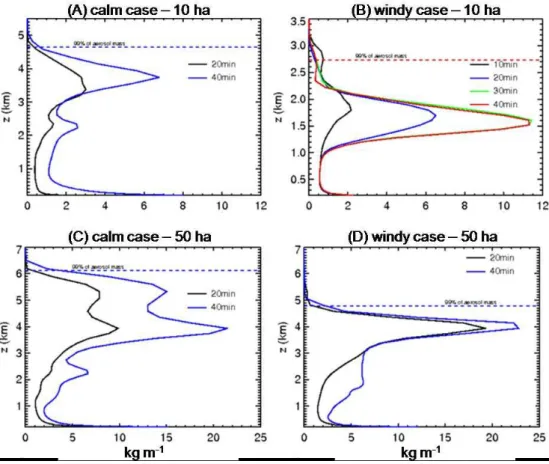
Fig. 3. Horizontally averaged vertical aerosol mass profile (kg m−1) as simulated by the ATHAM model for the calm(A),(C)and windy (B),(D)cases. Model results for a fire with size of 10 ha (A, B) and 50 ha (C, D). Note that the vertical axis uses different ranges for the heightz.
in the windy case near 4 km, while the aerosol is spread be-tween 4 and 6 km in the calm case. In both cases, the at-mospheric stability is lower in the windy case, so the plume should be higher, but due to lateral wind effects it is bended to the side, at the expense of vertical motion with stronger mixing with the ambient air properties.
3.3 Model results of 1-D PRM runs and comparison with ATHAM simulations
In this section 1-D PRM model results are discussed and compared with the 3-D ATHAM simulations. In order to compare the results from PRM to those from ATHAM, we introduced the parameter vertical mass distribution (VMD) which is parameterized from the vertical wind profile simu-lated by PRM model (see Appendix B). The way this quan-tity is defined provides the injection layer estimated by the 1-D simulation. Obviously, the injection layer is not explicitly simulated in 1-D model as it is in 2-D or 3-D cloud resolving models such as ATHAM and needs to be parameterized. The VMD provides a probability vertical mass distribution as a function of the simulated 1-D vertical velocity profile.
3.3.1 Smaller fires –10 ha size
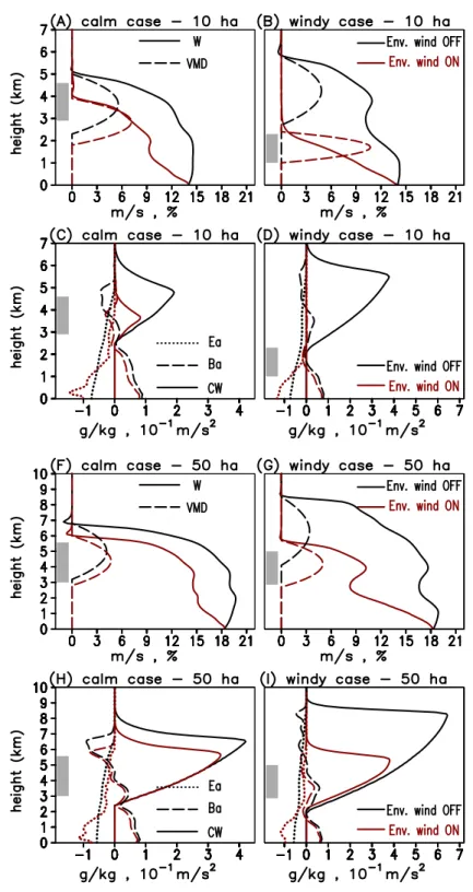
Figure 4a and b show the 1-D PRM model steady state solu-tions in the calm and windy ambient cases, respectively. We assumed identical fires burning tropical forest areas with a heat flux of 80 kW m−2(as stated before) and a size of 10 ha under both ambient conditions. The vertical velocity (W, m s−1) and vertical mass distribution (VMD, %) profiles are shown. Both panels also introduce the model results consid-ering a no-wind hypothesis by settingue(z)=0, as described
in Sect. 3.1.
Fig. 4. 1-D PRM model results for the calm and windy cases. For the calm condition,(A)and(C)show the results for a fire size of 10 ha; while(F)and(H)refers to the 50 ha size. The results for the windy case are in(B)and(D)(10 ha) and(G)and(I)(50 ha). The quantities are: vertical velocity (W, m s−1), vertical mass distribution (VMD, %), entrainment acceleration (Ea, 10−1m s−2), buoyancy acceleration (Ba,
relative motion between the smoke plume and the ambient air, predicts a lower layer, with approximately the upper half inside the ATHAM injection layer and the lower half below that.
To better understand the role of the dynamic entrainment, we show at Fig. 4c the total condensate water (CW), buoy-ancy acceleration (Ba) and entrainment acceleration (Ea) for
the cases discussed before. CW is in mixing ratio (g kg−1) and refers to the total condensed water (liquid, rain and ice). The buoyancy and entrainment accelerations (m s−2) are de-fined respectively by:
Ba=
1
1+γgB (10)
Ea= −(λentr+δentr)w (11)
where the symbols on the right side were already defined before. The balance between these two terms provides the net vertical acceleration of the in-plume air parcels. With no dynamic entrainment in the model formulation, the plume is capped by a cumulus with a total condensate water of
∼2 g kg−1near 5 km height. Dynamic entrainment strongly reduces the cumulus properties, not only in terms of the total condensed water (maximum∼1 g kg−1) but also the cloud volume. In terms of the buoyancy acceleration, the dynamic entrainment reduces its magnitude due to enhanced entrain-ment of drier air. On the other hand, the entrainentrain-ment accel-eration is increased (in magnitude) in the lower levels, due to additional dynamic entrainment. At upper levels, the magni-tude of Ea decreases becauseδentr is smaller (sinceuis
ap-proximatelyue) and at the same time the lateral entrainment is smaller due the larger horizontal size of the plume. The net effect ofδentris to reduce the vertical velocity for the entire
plume column and its top height.
The windy ambient case is discussed as follows. Profiles of vertical velocity and vertical mass distribution are shown in Fig. 4b. In this case, the impact of the dynamic entrain-ment is greatly pronounced. Not taking account the drag by the horizontal ambient wind, results on a predicted plume top height at∼5.8 km with a VMD between 2.8 and 5.8 km by 1-D PRM. However, the plume top height predicted by ATHAM (Fig. 3b) was∼2.5 km with the aerosol mass de-trainment layer (represented at Fig. 4b by the grey rectan-gle) localized approximately between 1 and 2.3 km. In this case the predicted 1-D PRM plume top height and VMD totally disagree with the corresponding ATHAM model re-sults. On the other side, with the dynamic entrainment in-cluded, 1-D PRM predicts a much lower plume top height around∼2.6 km with VMD between 1 and 2.5 km, and now the agreement with ATHAM is significantly improved.
For this case, the condensed water and accelerations are shown in Fig. 4d. Because the ambient air is moister in the windy case, when comparing with the calm case, not in-cluding the dynamic entrainment, the plume is capped by a bigger cumulus with the CW of∼4 g kg−1at 5.5 km height.
However, because of the stronger deceleration caused by the windy environment and efficient mixing with drier and cooler ambient air, the plume is prevented to reach the lifting con-densation level. Consequently, there is no additional buoy-ancy gained from latent heat release which would induce further vertical displacement of the in-plume air parcels and higher plume top height. In this case, no clouds are formed at top of the plume (CW∼0). Both processes explain the much lower plume top height and injection layer presented in the windy case.
3.3.2 Bigger fires –50 ha size
The 1-D PRM model simulations for bigger fires are dis-cussed here. Figure 4f and i introduce the results for big-ger fires with size of 50 ha. All other settings remain the same as in the previous cases. The larger size of the fire promotes stronger updrafts and higher clouds tops, similar to ATHAM results. For the calm case, the vertical velocity and VMD profiles are shown in panel (f). The difference in the cloud top height caused by dynamic entrainment is about 1 km (from 7 to 6 km). The cloud top predicted by ATHAM (Fig. 3c) was∼6 km with the aerosol mass detrain-ment layer localized approximately between 3 and 5.8 km. The results of the 1-D PRM with the dynamic entrainment present a better agreement with ATHAM simulation in terms of the predicted cloud top as well as the injection layer height and depth, as described by the VMD quantity.
Figure 4g shows the results for the windy ambient case. As in the case of the 10 ha fire, including dynamic entrainment causes much larger changes in the simulated plume rise; the plume top height drops from 8.5 to 5.8 km, a difference of 2.7 km. The vertical mass distribution not including the dy-namic entrainment is centered at 6.5 km extending from 4 to 8.5 km. Due to the enhanced horizontal entrainment asso-ciated with relative motion between ambient and the plume, the vertical mass distribution center drops to 4.2 km extend-ing from 2.8 to 5.8 km. From ATHAM simulation (Fig. 3d), the predicted plume top of this case is around 4.9 km with the main detrainment aerosol layer localized between∼2.9 and 4.9 km. Therefore, similar to the calm case, including the dynamic entrainment results in a much better agreement with the 3-D model simulations. 1-D PRM results and dis-cussion of the simulated CW, Baand Eafor the 50 ha fire are
produced using the complex non-hydrostatic 3-D ATHAM model. Our findings suggest that the extended 1-D model can generate feasible simulations when compared to the 3-D model.
There are few observational data related to fires to be used to evaluate this 1-D PRM. So far, we identified two well doc-umented cases: the 1994 Quinault and 2001 Chisholm fires. Detailed studies comparing the performance of 1-D PRM on simulating the plume top and injection heights of these fires will appear on upcoming paper.
The new formulation, when embedded in 3-D regional or global transport models to determine the vertical mass detrainment layer of smoke associated to vegetation fires, should improve the simulation of vertical distribution, trans-port and dispersion of aerosols and trace gases, mainly in areas dominated by small fires, as in savannas, pasture or cropland, and/or in a windy environment where the dynamic entrainment processes dominate the plume-environment hor-izontal mixing.
The new information needed by the extended formulation is the horizontal ambient wind, which is routinely simulated by the large scale 3-D host models. Therefore this new fea-ture is easily implemented and the impact of wind-generated dynamic entrainment process on regional and global smoke distribution predicted. In addition, the vertical mass distri-bution provides a way that 1-D cloud models can simulate not only the cloud top but also the actual mass detrainment layers. These are the fundamental quantities needed to deter-mine the emission source field resulting of vegetation fires to be used in the 3-D host large scale transport models.
Appendix A
The dynamic entrainment formulation
Consider a cylindrical volume of radiusRand depth1z(see Fig. A1). The horizontal mass flux (fh)within the plume is
given by
fh=ρe(ue−u) (A1)
whereρeis the ambient air density andueanduwere defined
above. Therefore, the mass gained by this plume layer during
Fig. A1. The description of the dynamic entrainment rate formula-tion (picture taken by M. Welling).
the time1tis
1m=fh(2R1z)1t=ρe(ue−u)(2R1z)1t (A2)
The definition of the mass entrainment rate is
δentr=
1
m 1m
1t
= 1
π R21zρcloud
ρe(ue−u)(2R1z)1t
1t (A3)
whereρcloudis the in-cloud air density. Assuming that
ρcloud≈ρe, (A4)
we finish with the following expression for the dynamic en-trainment
δentr=
2
π R(ue−u). (A5)
Appendix B
The vertical mass distribution (VMD) definition
the in-plume vertical velocity starts to decrease (zi) until the level where it is less than 1 m s−1(z
f). Based on this
defini-tion, the vertical mass distribution is defined as follows: (a) from the 1-D PRM steady state vertical velocity profile,
the upper half part of the cumulus is determined in terms of the heightszi andzf (zf>zi);
(b) a parabolic function of the heightzwith roots atzi and zf is defined;
(c) the function is then normalized to 1 in the interval[zi, zf].
Acknowledgements. We acknowledge partial support of this work by CNPq (302696/2008-3, 309922/2007-0) and by the Max Planck Society (MPG). J. T. thanks Stephan Eto for conducting the ATHAM model simulations. The authors thank the anonymous reviewer for the constructive comments and helpful suggestions.
Edited by: Y. Balkanski
References
Bursik, M.: Effect of wind on the rise height of volcanic plumes, Geophys. Res. Lett., 28(18), 3621–3624, 2001.
Cunningham, P., Goodrick, S. L., Hussaini, M. Y., and Linn, R. R.: Coherent vortical structures in numerical simulations of buoy-ant plumes from wildland fires, Int. J. Wildland Fire, 14, 61–75, 2005.
Cunningham, P. and Linn, R. R.: Numerical simulations of grass fires using a coupled atmosphere-fire model: Dy-namics of fire spread, J. Geophys. Res., 112, D05108, doi:10.1029/2006JD007638, 2007.
Ernst, G. G. J., Davis, J. P., and Sparks, R. S. J.: Bifurcation of vol-canic plumes in a crosswind, Bull Volcanol, 56, 159–169, 1994. Freitas, S. R., Longo, K. M., and Andreae, M. O.: Impact of
includ-ing the plume rise of vegetation fires in numerical simulations of associated atmospheric pollutants, Geophys. Res. Lett., 33, L17808, doi:10.1029/2006GL026608, 2006.
Freitas, S. R., Longo, K. M., Chatfield, R., Latham, D., Silva Dias, M. A. F., Andreae, M. O., Prins, E., Santos, J. C., Gielow, R., and Carvalho Jr., J. A.: Including the sub-grid scale plume rise of vegetation fires in low resolution atmospheric transport models, Atmos. Chem. Phys., 7, 3385–3398, 2007,
http://www.atmos-chem-phys.net/7/3385/2007/.
Graf, H.-F., Herzog, M., Oberhuber, J. M., and Textor, C.: The ef-fect of environmental conditions on volcanic plume rise, J. Geo-phys. Res., 104(D20), 24309–24320, 1999.
Herzog, M., Oberhuber, J. M., and Graf, H.-F.: A Prognostic Tur-bulence Scheme for the Nonhydrostatic Plume Model ATHAM, J. Atmos. Sci., 60, 2783–2796, 2003.
Latham, D.: A one-dimensional plume predictor and cloud model for fire and smoke managers, General Technical Report INT-GTR-314, Intermountain Research Station, USDA Forest Ser-vice, November, 1994.
Luderer, G., Trentmann, J., Winterrath, T., Textor, C., Herzog, M., Graf, H. F., and Andreae, M. O.: Modeling of biomass smoke injection into the lower stratosphere by a large forest fire (Part II): sensitivity studies, Atmos. Chem. Phys., 6, 5261–5277, 2006, http://www.atmos-chem-phys.net/6/5261/2006/.
McCarter, R. and Broido, A.: Radiative and convective energy from wood crib fires, Pyrodinamics, 2, 65–85, 1965.
Oberhuber, J. M., Herzog, M., Graf, H.-F., and Schwanke, K.: Vol-canic plume simulation on large scales, J. Volcanol. Geotherm. Res., 87, 29–53, 1998.
Rose, W. I., Gu,Y., Watson, I. M., et al.: The February–March 2000 Eruption of Hekla, Iceland from a Satellite Perspective, in Vol-canism and Earth’s Atmosphere, Geophys. Monogr. Ser., 139, edited by: Robock, A. and Oppenheimer, C., 107–132, AGU, Washington, D. C., 2003.
Simpson, J. and Wiggert, S.: Models of precipitating cumulus tow-ers, Mon. Weather Rev., 97, 471–489, 1969.
Textor, C., Graf, H.-F., Herzog, M., and Oberhuber, J. M.: Injection of gases into the stratosphere by explosive volcanic eruptions, J. Geophys. Res., 108(D19), 4606, doi:10.1029/2002JD002987, 2003.
Textor, C., Graf, H. F., Herzog, M., Oberhuber, J. M., Rose, W. I., and Ernst, G. G. J.: Volcanic particle aggregation in explosive eruption columns, Part I: Parameterization of the microphysics of hydrometeors and ash, J. Volcanol. Geotherm. Res., 150, 359– 377, 2006.
Trentmann J., Andreae, M. O., Graf, H.-F., Hobbs, P. V., Ottmar, R. D., and Trautmann, T.: Simulation of a biomass-burning plume: Comparison of model results with observations, J. Geo-phys. Res., 107(D2), 4013, doi:10.1029/2001JD000410, 2002. Trentmann, J., Luderer, G., Winterrath, T., Fromm, M. D.,
Servranckx, R., Textor, C., Herzog, M., Graf, H.-F., and An-dreae, M. O.: Modeling of biomass smoke injection into the lower stratosphere by a large forest fire (Part I): reference sim-ulation, Atmos. Chem. Phys., 6, 5247–5260, 2006,
http://www.atmos-chem-phys.net/6/5247/2006/.