www.hydrol-earth-syst-sci.net/20/4929/2016/ doi:10.5194/hess-20-4929-2016
© Author(s) 2016. CC Attribution 3.0 License.
Age-ranked hydrological budgets and a travel time
description of catchment hydrology
Riccardo Rigon1, Marialaura Bancheri1, and Timothy R. Green2
1Dipartimento di Ingegneria Civile Ambientale e Meccanica, Universitá degli Studi di Trento, Trento, Italy 2USDA-ARS, Water Management and Systems Research Unit, Fort Collins, Colorado, USA
Correspondence to:Riccardo Rigon ([email protected])
Received: 4 May 2016 – Published in Hydrol. Earth Syst. Sci. Discuss.: 9 May 2016 Revised: 9 November 2016 – Accepted: 16 November 2016 – Published: 15 December 2016
Abstract.The theory of travel time and residence time dis-tributions is reworked from the point of view of the hydro-logical storages and fluxes involved. The forward and back-ward travel time distribution functions are defined in terms of conditional probabilities. Previous approaches that used fixed travel time distributions are not consistent with our new derivation. We explain Niemi’s formula and show how it can be interpreted as an expression of the Bayes theorem. Some connections between this theory and population theory are identified by introducing an expression which connects life expectancy with travel times. The theory can be applied to conservative solutes, including a method of estimating the storage selection functions. An example, based on the Nash hydrograph, illustrates some key aspects of the theory. Gen-eralization to an arbitrary number of reservoirs is presented.
1 Introduction
Hydrological travel times have been studied extensively for many years. Some researchers (Rodriguez-Iturbe and Valdes, 1979; Rinaldo and Rodriguez-Iturbe, 1996), as reviewed by Rigon et al. (2016), looked at the construction of the hydro-logic response using geographical information. Others (e.g., Uhlenbrook and Leibundgut, 2002; Birkel et al., 2014) used travel times to understand catchment processes in relation to tracer experiments, while new experimental techniques were being developed (e.g., Berman et al., 2009; Birkel et al., 2011).
Based on these premises, Fenicia et al. (2008), Clark et al. (2011), McMillan et al. (2012), and Hrachowitz et al. (2013) aimed to describe both the spatial organization of the
catch-ment and the set of interactions between processes with an assembly of coupled storages (reservoirs) in the number and the organization necessary to give proper hydrological results without adding unwanted parametric complexity (e.g., Kle-meš, 1986; Kirchner, 2006). Despite the simplification ef-forts, the process of adding physical rigor to their models led to quite complex systems. Travel time analysis became a tool to disentangle flux complexities (e.g., Tetzlaff et al., 2008), opening the way for explicit unification of geomorphic theo-ries and storage-based modeling (Rigon et al., 2016).
Subse-quently, Harman (2015b) reformulated the SAS to be a func-tion of the watershed storage and actual time.
These approaches opened the possibility of exploring the nature of storage–discharge relationships, which are usually parameterized within rainfall–runoff models, and can pro-vide fundamental insight into the catchment functions in-voked previously (e.g., Seibert and McDonnell, 2002; Kirch-ner, 2009). Also, the traditional work on groundwater flow and catchment-scale transport can be associated with the same ideas, but using time-invariant travel time distributions (e.g., Dagan, 1984). Instead, Botter et al. (2011) used an ap-proach that is inherently non-stationary and has immediately attracted the attention of researchers in that field (e.g., van der Velde et al., 2012; Cvetkovic et al., 2012; Cvetkovic, 2013; Ali et al., 2014). A more detailed history of these concepts can be found in Benettin et al. (2013). Appendix B includes a brief review that is more specifically related to the scope of the present paper. All of these studies provided valuable advances to the theory, but the literature remains obscured by different terminologies and notations, as well as by model assumptions that are not fully explained.
There remains a need for theoretical developments that are clearly explained and developed using a consistent set of no-tations. Questions arise, like does the theory contain hidden parts that are not consistent or explained well? How does it relate to the instantaneous unit hydrograph theory? How can it be used? What generates time-varying backward prob-abilities? Does the theory fully account for those phenomena which are involved in mobilizing old water (e.g., McDonnell and Beven, 2014; Rinaldo et al., 2015; Kirchner, 2016a)?
Questions also remain about how to apply the theory of age-ranked distributions in terms of the model form and pa-rameter estimation. Harman (2015a) noted the importance of selecting an appropriate SAS, but until very recently (Har-man, 2015b), there was no proposed method for selecting the form of an SAS and estimating it from available data. Se-lection of the SAS for a given watershed remains a topic of importance, since it should not be imposed arbitrarily.
Our work includes a short review of existing concepts that were collected from many (mostly theoretical) papers, which used different conventions and approaches. In the following sections, the theory to date is synthesized into a framework using consistent notation. Besides presenting the concept in a new and organized way, our paper contains some non-trivial answers to the above questions. Clarifications and extensions will be presented and summarized in an integrated manner. These conceptual developments are followed by improved methods for selecting the appropriate form of SAS and esti-mating its parameters. Guidance for hierarchical approaches to parameter estimation is given, based on available data. Fi-nally, the proposed framework and methods are illustrated using data from an experimental watershed.
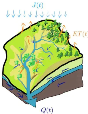
Figure 1.A single control volume is considered in which the fluxes are the total precipitation, evapotranspiration and discharge.
2 Definitions of age-ranked quantities
Residence time, travel time and life expectancy of water par-ticles and associated constituents flowing through watersheds are three related quantities whose meaning is well defined by the following equation:
T =(t−tin)
| {z } Tr
+(tex−t )
| {z }
Le
, (1)
whereT [T] ([T] means time units) is the travel time,t[T] is the actual time measured by a clock,tin[T] is the injection time (i.e., the time at which a certain amount of water en-ters the control volume), andtex[T] is the exit time (i.e., the time at which a certain amount of water exits the control vol-ume). Based upon these definitions,Tr:=t−tin[T] is the so-called residence time, or the age of water entered at timetin, andLe:=tex−t[T] is the life expectancy of the same water molecules which are inside of the control volume.
Consider, for example, a control volume such as the one shown in Fig. 1. Its (bulk) water budget is written as dS(t )
dt =J (t )−Q(t )−AET(t ), (2)
are modeled. Common simple estimates for the two latter quantities are
Q(t )=1
λS
b(t ) (3)
and AET(t )=
S(t ) Smax
E(t ), (4)
whereλ[T] andbare the parameters of the nonlinear reser-voir model,Smaxis the maximum water storage, andE(t )is the potential ET, temporal function of the radiation inputs, and atmospheric conditions. Assuming that radiation and various parameters used to model Q and AET are given,
Eq. (2) can be solved andS(t )obtained. If b=1, the bud-get is a linear ordinary differential equation, and its solution is analytic as in Coddington and Levinson (1955); otherwise, the solution can be obtained through an appropriate numeri-cal solver (e.g., Butcher, 1987). We made the simplification here to use a single storage for illustrative purposes. How-ever, extending the formalism to multiple storages is straight-forward, as shown in Appendix C.
Being interested in knowing the age of water, we need to consider a more general set of equations.
Assume that the water storage S(t ) can be decomposed into its sub-volumess(t,tin)[L3T−1] which refer to water injected into the system at timetin∈[0,tp]. Thus
Stp(t )=
min(t,tp)
Z
0
s (t, tin)dtin, (5)
where the initial timet=0 comes before any input into the control volume, andtprepresents the end of the last precip-itation considered in the analysis. The variable t represents the actual time at which the storage is considered. In the fol-lowing equations, the reference totpwill be dropped for no-tational simplicity, and any quantity will consider a limited time interval. The functional form ofs(t,tin), as well as the functions we define below, can vary witht andtin, so they should be labeled appropriately –s(t,tin)(t,tin)– but this has
been avoided to keep notations simple.
Analogously, Q(t ) [L3T−1] is the discharge out of the control volume, andq(t,tin)[L3T−2] is the part of the dis-charge exiting the control volume at timetcomposed of wa-ter molecules that enwa-tered at timetin∈[0,tp]:
Q(t )=
min(t,tp)
Z
0
q (t, tin)dtin. (6)
Actual evapotranspiration, AET(t )[L3T−1], is the sum of
its parts aeT(t,tin)[L3T−2] as
AET(t )=
min(t,tp)
Z
0
aeT(t, tin)dtin. (7)
Finally, letJ (t )[L3T−1] denote the input to the control vol-ume. This input can have an “age”, and therefore it can be defined as
J (t )= min(t,tp)
Z
0
j (t, tin)dtin. (8)
All these bivariate functions oft andtin,s(t,tin),q(t,tin), and aeT(t,tin)are null fort < tinand can present a derivative discontinuity at the origin (t=tin). Given the above defini-tions, we can rewrite the water budget as a set of age-ranked budget equations:
ds (t, tin)
dt =j (t, tin)−q (t, tin)−aeT(t, tin) . (9)
These equations were first introduced by van der Velde et al. (2012) and named by Harman (2015a), even though simi-lar ones were present in the previous literature, as discussed in Appendix B. In our formulation, however, by usingt and
tin instead oft andTr as independent variables, we do not need to transform the original ordinary differential equations (Eq. 9) into partial differential equations.
3 Backward and forward approaches
“Backward” and “forward” are well-known concepts in the study of travel time distributions. They were first introduced by Niemi (1977), then by Cornaton and Perrochet (2006), for example, and recently refined by Benettin et al. (2015). Benettin et al. (2015), in particular, related the backward con-cept to the residence time (or age), while the concon-cept of travel time is both forward or backward. However, according to us, these previous works did not fully disclose the inner mean-ing of the two concepts. In fact, in our theory, the probabili-ties are defined as backward when they “look” in time to the history of water molecules and forward when they “look” in time to their exit from the control volume. According to the previous statements, we can define a backward residence time probability, which is conditioned totand “looks” back-ward totin, and a forward residence time probability, which is conditioned totin and “looks” forward tot. In the same way, we can define a backward life expectancy probability, which is conditioned totex and “looks” backward tot, and a forward life expectancy probability, which is conditioned tot and “looks” forward totex. All these concepts will be clarified further in the following sections.
ps(Tr|t ), can be defined as
ps(Tr|t )≡pS(t−tin|t ):=
s (t, tin)
S(t ) h
T−1
i
, (10)
where “≡” means equivalence, and “:=” a definition. Benet-tin et al. (2015) denotedps(Tr|t )as
←
ps(Tr,t ), but since this probability density is conditional on the actual time, standard probability notation is clear and unambiguous.
It is evident that this probability is time-variant, since the integral and the integrand in Eq. (5) keep a dependence on the clock timet.
The pdf of “travel time” is pQ(t−tin|t ), where tex=t, since we are considering the water exiting the control vol-ume as discharge. It can be defined as
pQ(t−tin|t ):=
q (t, tin)
Q(t ) h
T−1i. (11)
This definition for the probability is very restrictive, and can imply inconsistencies in those papers which assume a time-invariant backward distribution to obtain a tracer concentra-tion as shown in Appendix D. Eventually, the pdf of travel time for water exiting the control volume as water vapor,
pET(t−tin|t ), can be defined as
pET(t−tin|t ):=
aeT(t, tin) AET(t )
h
T−1
i
. (12)
It is also possible to define the mean age of water for any of the two outlets, which is given by
hTr(t )ii=
min(t,tp)
Z
0
(t−tin) pi(t−tin|t )dtin (13)
fori∈ {Q, ET}, which is a function of the sampling time (and the rainfall input).
After the above definitions, the age-ranked equation (Eq. 9) can be rewritten as
d dt
S(t )ps(Tr|t )
=J (t )δ (t−tin)−Q(t )pQ(t−tin|t )
−AET(t )pET(t−tin|t ) , (14)
when a single “new water” injection of mass is considered, and the bulk quantitiesS(t ),Q(t ), and AET(t )are known as
soon as the bulk water budget, Eq. (2), is solved. δ(t−tin) is a Dirac-delta function to account for the water particles in precipitation with age zero. The travel time probabilities on the right side of Eq. (14) are not known. Consequently Botter et al. (2011) introduced a storage selection function,
ω(t,tin)(–), for each of the outputs that relate the travel times to the residence time, so that
pQ(t−tin|t ):=ωQ(t, tin) ps(Tr|t ) (15)
and
pET(t−tin|t ):=ωET(t, tin) ps(Tr|t ) . (16)
Therefore Eq. (14), after the proper substitutions, becomes d
dt
S(t )ps(Tr|t )=J (t )δ (t−tin|t ) −Q(t )ωQ(t, tin) ps(Tr|t )
−AET(t )ωET(t, tin) ps(Tr|t ) . (17) Once assigned the ω(t, tin) values on the basis of some heuristic, as in Botter et al. (2011), Eq. (17) represents a lin-ear ordinary differential equation and can be solved exactly as
ps(Tr|t )=e
−Rtt
ing(x,tin)dx
p(0|t )+ t Z
tin
J (y)δ (y−tin)
S(y) e
Rt
ting(x,tin)dxdy
(18)
where
g (x, tin)= 1
S(x)
dS(x)
dt +Q(x)ωQ(x, tin)
+AET(x)ωET(x, tin)] (19)
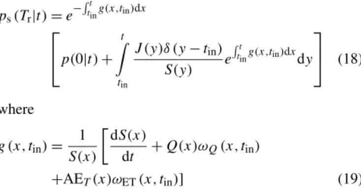
and p(0|t ) is the initial condition. This is only valid if Eq. (17) is linear, i.e.,ω(t,tin)is not a function ofps(Tr|t ). Figure 2 shows the variation of theps(Tr|t )with the injection time, while the chronological time is kept fixed. The curves were obtained considering three different injections attin1,
tin2, andtin3, and assumingωQ(t,tin)=ωET(t,tin)=1.
The conditional probabilityps(Tr|t )properly integrates to one, as shown in Fig. 3, when it is integrated intin. In par-ticular, Fig. 3 shows thatps(Tr|t )is constant whenJ (t )=0. In fact, if we considerωQ(t,tin)=ωET(t,tin)=1, Eq. (17) is simplified in
d dt
S(t )ps(Tr|t )
= −Q(t )ps(Tr|t )−AET(t )ps(Tr|t ) (20) and, therefore,
dps(Tr|t ) dt = −
ps(Tr|t )
S(t )
dS(t )
dt −Q(t )−AET(t )
=0. (21)
Figure 4 shows the evolution ofps(Tr|t ) with the actual timet and the injection time kept fixed. The integral of the area under the three curves, obtained for the same three in-jections, in this case, is not equal to 1, since the functions are not pdfs int.
5 Response time (forward probabilities)
0.00 0.01 0.02 0.03 0.04
Injection time tin
Pro
b
a
b
ili
ty,
p
S
[t
-tin
|t]
ti
n1
t
in2 tin3
Figure 2.Representation of the evolution of the backward pdf for three injection times (tini, wherei=1, 3) as varying with the
in-jection time tin. The time shift between the three injections was
dropped for a direct comparison of the curves.
0.00
0.25 0.50
0.75 1.00
Injection time tin
C
u
mu
la
ti
ve
d
ist
ri
b
u
ti
o
n
f
u
n
ct
io
n
,
PS
[t
-tin
|t] tin1
tin2
ti
n3
Figure 3.Representation of the backward cumulative distribution function for three injection times (tini, wherei=1, 3) as varying
with the actual timet. The time shift between the three injections was dropped for a direct comparison of the curves.
catchment, we can write its integral form over dtas
s (t, tin)=J (tin)−
t Z
0
q (t, tin)dt−
t Z
0
aeT(t, tin)dt. (22)
It can be rewritten as a probability conditional ontin,
Ps[t−tin|tin]:=1−
s (t, tin)
J (tin)
=VQ(t, tin)
J (tin)
+VAET(t, tin)
J (tin)
,
(23)
0.000 0.005 0.010 0.015 0.020
Actual time t
Pro
b
a
b
ili
ty,
p
S
[t
-tin
|t]
ti n1
tin2
t in3
Figure 4. Representation of the evolution of the backward pdf vs. the actual timet. The time shift between the three injections was dropped for a direct comparison of the curves. In this case, the area below the curves is not equal to 1.
called “forward residence time” probability distribution, hav-ing defined
VQ(t, tin):=
t Z
0
q (t, tin)dt (24)
and
VAET(t, tin)=
t Z
0
aeT(t, tin)dt. (25)
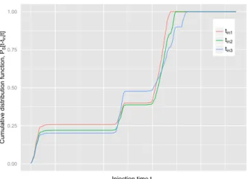
Ps[t−tin|tin], as shown in Fig. 5, varies (with t), as ex-pected, between 0 and 1 and has density
ps(t−tin|tin)= − 1
J (tin)
ds (t, tin)
dt =
q (t, tin)
J (tin)
+aeT(t, tin) J (tin)
. (26)
It can be observed instead that
F(t−tin|tin):=
VQ(t, tin)
J (tin)
(27) and
G(t−tin|tin):=
VAET(t, tin)
J (tin)
0.00
0.25 0.50 0.75 1.00
Time
F
o
rw
a
rd
p
ro
b
a
b
ili
ty
d
ist
ri
b
u
ti
o
n
,
PS
[t
-tin |tin
]
s(t,tin)
PS[t-tin|tin]
F
Figure 5.Forward residence time probability distribution: in red the relative storage, in green the forward residence time distribution and in blue the relative discharge function.
In order to normalizeFandG, the asymptotic value of the
partitioning coefficient is defined among theQand ET:
2 (tin):= lim
t→∞2 (t, tin):=t→∞lim
VQ(t, tin)
VQ(t, tin)+VAET(t, tin)
. (29)
Then, it is easy to show that
pQ(t−tin|tin):=
q (t, tin)
2 (tin) J (tin)
(30) and
pET(t−tin|tin):=
aeT(t, tin)
(1−2 (tin)) J (tin)
(31) are the forward probability density functions of discharges and evapotranspiration, which properly normalize to 1 when integrated overt. The two probability density functionspQ
andpETare related through
ps(t−tin|tin)=2pQ(t−tin|tin)+(1−2)pET(t−tin|tin) . (32) Unlike backward probabilities, the forward probabilities de-scribe how a catchment reacts to precipitation events, but they do not describe the actual time the water takes to move through the catchment. To avoid confusion, the expected value of a travel time, weighted by the forward distribution, will be called the mean “response time” (instead of mean travel time). For discharge, the result is
Q(t )=
min(t,tp)
Z
0
pQ(t−tin|tin) 2 (tin) J (tin)dtin, (33)
which can be seen as a generalization of the instantaneous unit hydrograph (IUH).
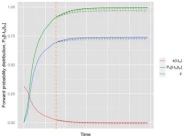
Figure 6.Representation of the forward probability of the outputs: in red the relative storage,s(t,tin), in green the output probability,
Ps[t−tin|tin], and in blue the relative discharge functionF, defined
in the text. The difference betweenPs[t−tin|tin]andFis the
func-tionG, defined in the text. The orange dashed line represents the generic instantt, after whichPs[t−tin|tin]andFare unknown.
Although2 may be unknown at any finite time, the ac-tual state of the system is obtained by solving the budget equation. More information and details on this partitioning coefficient are provided in the next section.
6 The partitioning coefficient2
2(tin)has been introduced to complete the algebra of prob-abilities in the presence of more than one outflow. However, estimation of the coefficient is important by itself, because it summarizes the relevant partitioning of hydrologic fluxes.
The first plot in Fig. 7 shows a time series of 2(t, tin) values obtained from a single injection time considering the complete mixing case (ωQ(t, tin)=ωET(t, tin)=1). Data used for the simulation are from Posina River, a small catch-ment in the northeastern part of the pre-alpine mountains in the Veneto region, Italy. At the beginning2(tin)(Fig. 7, top panel) shows large oscillations due to hourly and daily os-cillations, especially in evapotranspiration. Because2(tin)is defined through integrals, these oscillations are progressively damped and become irrelevant after a couple of weeks (when discharge is still higher than baseflow, as appears from the age-ranked discharge in Fig. 7, bottom panel).
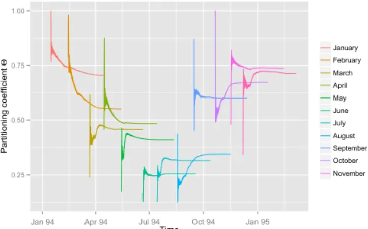
Figure 8 shows different time series of the partitioning co-efficient: each curve represents the time evolution of 2(t,
0.5 0.6 0.7 0.8 0.9 1.0
Gen Feb Mar Apr Mag Giu
Time
Pa
rt
it
io
n
in
g
co
e
ff
ici
e
n
t
Θ
0e+00 2e-04 4e-04 6e-04 8e-04
Gen Feb Mar Apr Mag Giu
Time
q
(t
,tin
)[m
m
h
]
3
-1
Figure 7.Variation of the partitioning coefficient in time, for a sin-gle injection time in January: after a timescale of 5 months its os-cillation became irrelevant and its value tended to its final value of 0.78.
were obtained in the summer months, with a minimum in June around 0.25.
7 Niemi’s relation
As a result of definitions made in Sects. 4 and 5, two relations exist involving q(t,tin), i.e., Eqs. (11) and (30), and aeT(t,
tin), i.e., Eqs. (12) and (31). Equating the two corresponding expressions results in
Q(t )pQ(t−tin|t )=2 (tin) pQ(t−tin|tin) J (tin) (34) and
AET(t )pET(t−tin|t )=[1−2 (tin)]pET(t−tin|tin) J (tin) , (35) wheret=texsince we are considering the particles leaving the control volume as discharge and evapotranspiration. The above relations are known in the literature as Niemi’s rela-tions or formulas, after Niemi (1977).
Defining the total volume of water injected in the system in [0,tp],
VS tp:= mint,tp
Z
0
J (tin)dtin= mint,tp
Z
0
(Q(t )+AET(t ))dt (36)
it can be observed that
pJ(tin):=
J (tin)
VS tp
(37)
can be considered the marginal pdf of the injection times, or the fraction of precipitation at a certain discrete tinwith
re-0.25 0.50 0.75 1.00
Gen 1994 Apr 1994 Lug 1994 Ott 1994 Gen 1995
Time
Pa
rt
it
io
n
in
g
co
e
ff
ici
e
n
t
Θ
January
February
March
April
May
June
July
August
September
October
November
Jan 94 Apr 94 Jul 94 Oct 94 Jan 95
Figure 8. Evolution of the partitioning coefficient in 1 year of hourly simulation: the highest values are achieved in January, with the lowest in June. However, the figure does not represent a simple oscillation. The March coefficient is lower than April. October and November present almost the same value.
spect to the total precipitation over a period of [0,tp]. Anal-ogously
pQ(t ):=
Q(t ) 2 (tin) VS(tin)
(38) is the marginal pdf of the outflow as discharge, or the fraction of discharge at a certaint generated by precipitation in the same [0,tp]. Then, Niemi’s relation (Eq. 34) becomes
pQ(t−tin|t ) pQ(t )=pQ(t−tin|tin) pJ(tin) , (39) which has the form of the well-known Bayes theorem. This shows that the interpretation of the backward and forward probabilities as conditional ones is fully consistent. On the other hand, this reveals that the joint probability ofTr and
tis
ps(Tr, t )=pQ(t−tin|t ) pQ(t )=pQ(t−tin|tin) pJ(tin) . (40)
Because the future is unknown, as remarked in Sect. 5, there should be a working Niemi relation for any finite timet
which does not require the knowledge of the asymptotic value2(tin). This can be easily derived after having defined
g (t−tin|tin):=
aeT(t, tin)
J (tin) ≡dG
dt (41)
and
f (t−tin|tin):=
q (t, tin)
J (tin) ≡dF
dt . (42)
From these definitions,
and
aeT(t, tin)=g (t−tin|tin) J (tin) (44)
and, therefore,
Q(t )pQ(t−tin|t )=f (t−tin|tin) J (tin) (45)
for discharges, and
AET(t )pAET(t−tin|t )=g (t−tin|tin) J (tin) (46) for evapotranspiration.
As a byproduct, the SAS and the forward functions are shown to be related. For discharge at any timet, for example,
f (t−tin|tin)=
Q(t )ωQ(t, tin) ps(t−tin|t )
J (tin)
. (47)
8 Residence times, travel times and life expectancy The forward probabilities can be related to the life ex-pectancy, i.e., the expected time the water molecules remain in the storage.
In the control volume, we can conceptually denote the sub-sets of the storage which contains the water molecules ex-pected to exit at timetexas
stex(t, tex) . (48)
Analogously to what was done before, we can observe that the quantity
ps(tex−t|t ):=
stex(t, tex)
S(t ) (49)
has the structure of a probability density function once inte-grated over alltexs, and it is reasonable to call it the proba-bility density of storage “life expectancy” for particles in the control volume at timet.
However,ps(tex−t|t )can also be related to the forward probabilities discussed in the previous section. In fact, it can be observed that the probability of storage-life expectancy satisfies the following relation to the age-ranked forward quantities:
stex(t, tex)=
min(t,tp)
Z
0
q (tex, tin)+aeT(tex, tin)
dtin
− min(t,tp)
Z
0
q (t, tin)+aeT(t, tin)
dtin, (50)
where, according to the definitions, min(t,tp)
Z
0
q (tk, tin)+aeT(tk, tin)
dtin
= min(t,tp)
Z
0
2 (tin) pQ(tk−tin|tin)
+(1−2 (tin)) pAET(tk−tin|tin)
J (tin)dtin. (51) The variabletk, used to make the equations above and below
more concise, is such thatt0=tex(k=0) andt1=t (k=1). The integral spans the time interval up totpbecause we are considering the storage derived for precipitation in the fi-nite interval [0,tp]. In Eq. (50) the equality says that the life storage at timet is equal to the water injected for any time
tin∈[0,tp], which is expected to exit as discharge or evap-otranspiration at timetex. The water still inside the control volume at clock timetis, however, all the water that entered the volume up to timet, minus the water that already flowed out.
This integral is not effectively known at timet, because what is happening between timet andtexis unknown, and so are the pdfs (as in Fig. 5), unless they are specified from some educated guess, as made in the last section of this paper. It follows that
ps(tex−t|t )=
S(t )−1 1 X
k=0
(−1)k min(t,tp)
Z
0
2 (tin) pQ(tk−tin|tin)+(1−2 (tin)) pAET(tk−tin|tin)
J (tin)dtin.
(52) Thus, the relation between the storage-life expectancy and the previously introduced backward and forward probabili-ties is mediated by an integral equation.
9 Passive and reactive solutes
The formalism developed in Sects. 2 to 6 applies in principle to any conservative substance, indicated by a superscripti. Therefore we have a bulk budget equation for the mass of the substanceiand an age-ranked budget for the same substance: dSi(t )
dt =J
i(t )−Qi(t )+Ri(S(t )) (53)
and dsi(t, tin)
dt =j
i(t, t
(in this case, three):
CSi(t ):=S i(t )
S(t ) (55)
for the concentration in storage,
CJi(t ):=J i(t )
J (t ) (56)
for concentration in input, and
CQi (t ):=Q i(t )
Q(t ) (57)
for discharges. The latter is actually the one which is usu-ally covered in the literature, since it is the one measured at the outlet of a control volume/catchment. For the solute dis-charge, an integral expression like
Qi(t )= min(t,tp)
Z
0
2 (tin) pQ(t−tin|tin) Ji(tin)dtin (58)
is assumed to be valid, where thei has been dropped from the probability distribution function, assuming that a passive solute moves with the water. Dividing Eq. (58) by the water discharge,
CQi (t )= min(t,tp)
Z
0
2 (tin) pQ(t−tin|tin)
Q(t ) J
i(t
in)dtin (59)
is obtained and, finally, applying Niemi’s formula,
CQi (t )= min(t,tp)
Z
0
pQ(t−tin|t )
Ji(tin)
J (tin) dtin
= min(t,tp)
Z
0
pQ(t−tin|t ) CJi (tin)dtin. (60)
Therefore the concentration of the passive solute in dis-charge is known once the concentration of the solute in input is known together with the backward probability (Rinaldo et al., 2011). The concentration estimated in this way groups substances injected at any time, in agreement with measure-ment practices. When a sample is taken, the action implies perfect mixing of all the age-ranked waters in the volume where measurements are made.
The bulk substance budget can instead be written as dSi(t )
dt =
dCSi(t )S(t )
dt =J
i(t )−Qi(t )+Ri(S(t ))
=Ji(t )−CQi (t )Q(t )+Ri(S(t )) (61)
and the missing concentrationCSi(t )can be easily estimated with the help of Eq. (55) sinceS(t )is also known.
The above is essentially the same as Eq. (12) in Duffy (2010), but the age-ranked formalism can be used to un-derstand a little more about the processes in action. Start-ing from the quantities that appear in Eq. (54), the backward probability can be defined as
piS(t−tin|t ):=
si(t, tin)
Si(t ) (62)
and analogous definitions (e.g., Eq. 11) can be given for the discharge and the inputs, so as to obtain, after the appropriate substitutions,
d dtC
i
S(t )S(t )ps(t−tin|t )=Ji(t )δ (t−tin) −CQi (t )Q(t )ωQ(t, tin) ps(t−tin|t )
| {z }
pQ(t−ti|t )
+ri(t, tin) , (63)
which is the master equation (Eq. 17) for the substance i. Many of the superscripts i were dropped, because the i -substance does not modify the velocity (i.e., it behaves like water).
The braces were added to emphasize that pQ(t−tin|t ) should have been left, and we could solve the system of equations directly forps(t−tin|t )andpQ(t−tin|t ), obtain-ing eventually the age-ranked quantities, usobtain-ing Eq. (53).
In fact, in Eq. (63) all the quantities are known, either be-cause of a solution of the solute budget Eq. (53) or the wa-ter maswa-ter equation (Eq. 17), or a known input (J (t )). The only quantity that is unknown (and usually guessed) isωQ(t,
tin). However, Eqs. (63) and (17) can be seen as two coupled equations inps(t−tin|t )andωQ(t,tin), and we can conclude that the SAS can be derived rather than imposed.
From a practical point of view there could be some ob-stacles in the correct determination of the SAS, because the distribution of the input of the substance can be unknown. In this case Eq. (63) can be used to back-trace the passive solute injection, after having made educated guesses on the SAS. In the presence of more than one solute, the flow of every solute obeys the same probabilitiespsandpQ. This redundancy can
then be used for improving their estimation by applying the appropriate statistical techniques.
For the sake of simplicity we neglected evapotranspiration. However, now that the concepts are established, we can ob-serve that incorporating AET involves a second SAS, which
remains undetermined. Various approaches can be chosen to overcome this fact. For instance, it can be assumed thatωQ(t,
Duffy (2010), as in Carrera and Medina (1999), added an equation for water age similar to our Eqs. (53) and (63). This is necessary when dealing with spatially distributed prop-erties (see Appendix B), but not at our spatially integrated scales. In fact, in our case, water age can be estimated di-rectly from its definition (Eq. 13), since the probability dis-tribution of residence time is known.
Finally, in order to clarify this theory, an example of ri
could be
ri(t, tin):=k1
si(t, tin)−k2seqi
, (64)
wherek1andk2are suitable reaction constants andseqi rep-resents an equilibrium storage. Whilst more complex reac-tions can be envisioned, this type of reaction (or sink term), being linear, does not alter the essential traits of the theory described above.
10 A simple example where probabilities are assigned instead than derived
With the scope to further clarify the formalism, we assume in this section that the forward pdfs introduced in the previous sections are known. We use the concept of linear reservoir, which has a long history in surface hydrology, e.g., Dooge (1973).
First consider only one outflow: the bulk equation for the water budget of a single linear reservoir is
dS(t )
dt =
n X
tin=1
Rtin−
1
λS(t ), (65)
where it has been assumed, for simplicity, that
J (t )= n P
tin=1
Rtin, i.e., that the precipitation is accounted
for as a sequence of instantaneous impulses at different timestins. By definition of the linear reservoir,
Q(t )=1
λS(t ), (66)
whereλ[T] is the mean response time (not to be confused with the mean “travel time” derived from the backward dis-tributions) in the reservoir. If this is the case, assuming that the age-ranked storages behave linearly, the age-ranked wa-ter budgets can be written as
ds (t, tin)
dt =Rtinδ (t−tin)−
1
λs (t, tin) , (67)
where it is
q (t, tin)= 1
λs (t, tin) . (68)
Equation (67), after integration overtin, reduces to Eq. (65). By definition, it iss(t,tin)=0 fort < tin, and the solution for
t > tinis well known as
s (t, tin)=Rtine
tin−t
λ . (69)
The equivalent solution, forS(t ), gives
S(t )=
t Z
tin
Rtine
−(t−tin)/λdt
in, (70)
and the backward probability can then be written as
ps(t−tin|t )=
Rtine
t−tin
λ
t R
tin
Rtine−(t−tin)/λdtin
. (71)
If and only ifRtinis a constant, the probability simplifies, and
it is time-invariant, i.e., dependent only on the residence time
Tr=t−tin. Please note that, in this case, we did not appeal to Eq. (17) to estimate the backward probability. Instead, in Eq. (71), we used the definitions.
Because discharges are just linearly proportional to the storage, it is easy to show that pQ(t−tin|t )=ps(t−tin|t ) and, therefore, in this case, ω(t, tin)=1. This shows that for the linear reservoir case, where for all injection times the mean residence time is equal (toλ), the SAS function is nec-essarily unitary. However, a more general case can be set if the mean residence time is a function oftin, meaning that Eq. (67) can be modified into
ds (t, tin)
dt =Rtinδ (t−tin)−
1
λtin
s (t, tin) , (72)
and its solution fort > tinis the same as Eq. (69), but with
λmuted intoλtin. However, due to the dependence ofλtinon
the injection time, the SAS is not a constant any more, being equal to
ωQ(t, tin):=
pq(t−tin|t )
ps(t−tin|t ) =λ−t 1
in
t R
tin
Rtine
−(t−tin)/λtindt in
t R
tin
λ−tin1Rtine
−(t−tin)/λtindtin
=λ−t 1
in
t R
tin
Rtine
+tin/λtindtin
t R
tin
λ−t1
inRtine
tin/λtindt in
. (73)
This seems to suggest that imposing the characteristics of the forward pdf could completely determine theωQ(t,tin). Vice versa, as already known, assigningωQ(t,tin)from some heuristic, obviously, would determine a mean residence time dependence on the injection time.
Even if semi-analytical results are not feasible using non-linear reservoirs, suitably tuning the parameters of each age-ranked equation cannot change the form of the SAS, as is also suggested by arguments below.
Other aspects come into play when there are multiple out-puts. Expanding the previous linear case to include evapo-transpiration, the bulk equation becomes
dS(t )
dt =
n X
tin=1
Rtin−
1
λ−aet(t )
S(t ), (74)
where the actual evapotranspiration is assumed to equal
AET(t )=S(t )aet(t ) (75)
with a linear dependence on the soil water content, as for instance in Rodriguez-Iturbe et al. (1999). The equations of water budget for the generations becomes
ds (t, tin)
dt =Rtinδ (t−tin)−
1
λtin
+aet(t, tin)
s (t, tin) ,
(76) where the bivariate dependence of aet(t, tin) on the actual time and the injection time can be justified by arguing that water of different ages is not perfectly mixed in the control volume and plant roots sample water of different ages in dif-ferent modes, according to their spatial distributions. Since Eq. (76) remains a linear ordinary differential equation, it can be solved analytically, and
s (t, tin)=Rtine
−3(t,tin) (77)
where
3 (t, tin):=
t Z
tin
1
λtin
+aet t′, tin
dt′ (78)
and
S(t )=
t Z
0
Rtine
−3(t,tin)dt
in. (79)
Notably, the outflow terms can be expressed as a function of the storage:
q (t, tin)+aet(t, tin)=µ (t, tin) s (t, tin) . (80)
The problem remains linear and analytically solvable. The quantity µ(t, tin) is usually called the age and mass-specific output rate (Calabrese and Porporato, 2015). Solving Eq. (76), it is not even necessary to show that
ωET(t, tin)6=1. (81)
The latter condition is regained if and only if aet(t,
tin)=aet(t); i.e., it depends only on the current time (which
is a condition that requires the perfect mixing of aged wa-ters). In fact, in case a dependence ontinremains, then trivial algebra says that
pET(t−tin|t )=
aet(t, tin) s (t, tin)
t R
tin
aet(t, tin) s (t, tin)dtin
, (82)
which implies
ωET(t, tin):=
pET(t−tin|t )
ps(t−tin|t )
=
aet(t, tin)
t
R
tin
Rtine−3(t,tin)dtin
t
R
tin
aet(t, tin) S (t, tin)dtin
.
(83) Obviously these results, obtained by imposing a travel time probability, can be inconsistent with tracer results, because both approaches impose a specific estimate of theω func-tions.
11 Conclusions
We reviewed existing concepts that were collected from many different papers, and presented them in a new system-atic way. We established a consistent framework that offers a unified view of the travel time theories across surface water and groundwater.
It contains several clarifications and extensions. Clarifications include the following.
– The concepts of forward and backward conditional probabilities and a small but important change in no-tation.
– Their one-to-one relation with the water budget (and the age-ranked functions) from which the probabilities were derived (after the choice of SASs).
– The proper way to choose backward probabilities. Specifically, it was shown that the usual way to assign time-invariant backward probabilities is inappropriate. We also show how to do it correctly, and introduced a minimal time variability.
– The fact that time-invariant forward probabilities usually imply time-varying backward probabilities, i.e., travel time distributions.
– The rewriting of the master equation by Botter, Bertuzzo, and Rinaldo as an ordinary differential equa-tion (instead of a partial differential equaequa-tion).
– The significance of the SAS functions with examples. – The relationship of the present theory with the
well-known theory of the instantaneous unit hydrograph. – We added information and clarified some links of the
present theory with Delhez et al. (1999) and Duffy (2010), as shown in Appendix B.
Extensions include
– new relations among the probabilities (including the re-lation between expectancy of life and forward residence time probabilities);
– an analysis of the partitioning coefficients (which are shown to vary seasonally);
– an explicit formulation of the equations for solutes which would permit direct determination of the SAS on the basis of experimental data;
– tests of the effects of various hypotheses, e.g., assum-ing a linear model of forward probability and a gamma model for the backward probabilities;
– an extension of Niemi’s relation (and a new normaliza-tion);
– the presentation of Niemi’s relation as a special case of the Bayes theorem; and
– a system of equations from which to obtain the SAS experimentally.
The extension of the theory to any passive substance diluted in water clearly opens the way to new developments of the theory and applications of tracers.
Finally, as a proof of concept, this paper includes exam-ples derived from a real case (Posina River basin) and comes with open-source code that implements the theory, available to any researcher (see Appendix E).
12 Data availability
Appendix A: Symbols, acronyms, and notation
Symbol Name Dimensions
aeT(t,tin) age-ranked evapotranspiration L3T−2
aeT(t,tex) exit time-ranked evapotranspiration L3T−2
b exponent of the nonlinear reservoir model –
f (t−tin|tin) time derivative of the relative discharge function T−1
fup partitioning coefficient between upper and saturated reservoirs –
g(t−tin|tin) time derivative of the relative evapotranspiration function T−1
g(Tr) incomplete Gamma distribution T−1
j (t,tin) age-ranked rainfall rate L3T−2
ji(t,tin) age-ranked input of the substancei L3T−2
k1,2 reaction’s constants –
piS(t−tin|t ) travel time backward pdf of the substancei T−1
pET(t−tin|t ) forward evapotranspiration pdf T−1
pET(t−tin|tin) forward evapotranspiration pdf T−1
pJ(tin) marginal pdf of the outflow as discharge –
plow(t−tin|t ) travel time backward pdf of the lower storage T−1
pQ(t−tin|t ) travel time backward pdf T−1
pQ(t−tin|tin) travel time forward pdf T−1
pQ(tin) marginal pdf of the injection times –
ps(Tr|t ) residence time backward pdf T−1
ps(t−tin|tin) residence time forward pdf T−1
ps(tex−t|t ) life expectancy backward pdf T−1
psat(t−tin|t ) travel time backward pdf of the saturated storage T−1
psup(t−tin|t ) travel time backward pdf of the upper storage T−1
q(t,tin) age-ranked discharge L3T−2
q(t,tex) exit time-ranked discharge L3T−2
qi(t,tin) age-ranked output of the substancei L3T−2
qlow(t,tin) age-ranked discharge for the lower reservoir L3T−2
qsat(t, tin) age-ranked discharge for the saturated reservoir L3T−2
ri(t,tin) age-ranked sink/source term L3T−2
s(t,tin) age-ranked water storage L3T−1
si(t,tin) age-ranked water storage of the substancei L3T−2
seqi equilibrium storage L3T−1
sex(t,tex) exit time-ranked discharge L3T−1
slow(t,tin) age-ranked water storage for the lower reservoir L3T−1
sup(t,tin) age-ranked water storage for the upper reservoir L3T−1
ssat(t,tin) age-ranked water storage for the saturated reservoir L3T−1
t actual time T
tex exit time T
tin injection time T
tp time of the end of the last precipitation considered in the analysis T
AET(t ) actual evapotranspiration L3T−1
CJi(t ) concentration in input –
CSi(t ) concentration in storage –
CQi (t ) concentration in discharge –
E(t ) potential evapotranspiration L3T−1
F(t−tin|tin) relative discharge function –
G(t−tin|tin) relative evapotranspiration function –
J (t ) rainfall rates L3T−1
Ji(t ) input rates of the substancei L3T−1
Symbol Name Units
Ps(t−tin|tin) forward residence time probability function –
Le life expectancy T
T travel time T
Tr residence time T
S(t ) volume of water stored in a control volume L3
Q(t ) discharge L3T−1
Qi(t ) output rates of the substancei L3T−1
Q1 recharge to the saturated reservoir L3T−1
Ql runoff produced by the lower reservoir L3T−1
Qsat outflow from the saturated storage L3T−1
Ri(S(t )) sink/source term L3T−1
R(t ) recharge to the lower reservoir L3T−1
R(t,tin) input to the lower reservoir L3T−1
Rtin sequence of instantaneous impulses at differenttins L
3
Si(t ) stored mass of the substanceistored L3
Slow storage in the lower reservoir L3
Smax maximum value of the storage L3
Ssat amount of water stored in the saturated storage L3
Sup storage in the upper reservoir L3
VAET(t,tin) time integral of the age-ranked evapotranspiration L3T−1
VS(tp) total volume injected in the volume in[0,tp] L3T−1
VQ(t,tin) time integral of the age-ranked discharge L3T−1
α coefficient of the gamma distribution –
δ(t−tin) Dirac-delta distribution T−1
γ coefficient of the gamma distribution –
λ coefficient of the nonlinear reservoir model T
µ(t,tin) age and mass-specific output rate –
ωET(t,tin) SAS for evapotranspiration –
ωlow(t,tin) SAS for runoff produced by the lower reservoir –
ωQ(t,tin) SAS for discharge –
ωQ1(t,tin) SAS for the recharge to the saturated reservoir –
ωR(t,tin) SAS for the recharge to the lower reservoir –
ωQsat(t,tin) SAS for runoff produced by the saturated storage –
2(tin) partitioning coefficient –
Appendix B: A little critical review of contributions on age-related equations
Without the need to be comprehensive, since some reviews of the topic were recently made available (Benettin et al., 2013; Hrachowitz et al., 2016), we believe it could be useful to summarize the contributions of some milestone papers in relation to ours. We choose here those references that have a direct theoretical influence, and leave out those already cited in the main text having more relevance in connection with experimental research and model identification. We also do not mention Dagan’s important work that we already com-mented on in Sect. 1.
We also do not mention travel time theories which emanate from the instantaneous unit hydrograph, since they were ex-tensively discussed in Rigon et al. (2016). The formal center of this paper’s contribution is Eq. (9). Being substantially a mass budget, it can be argued that it has been central in many scientific disciplines and hydrology’s sub-disciplines. How-ever, as stated in the main text, van der Velde et al. (2012) is the first contribution where the equation appears in the form we use.
One of the older papers on this subject is Campana (1987), who wrote an equation for water age distribution, but he used a discrete time formalism that is not easily translatable into our derivation. The remarkable work of Carrera and Med-ina (1999) paid direct attention to the question of water ages by finding one partial differential equation (pde) for the resi-dence time distributions and one pde for water ages. A sim-ilar approach was also followed by Ginn (1999). Their con-tributions fall in the area of advection–dispersion types of equations and were implemented almost at the same time in Delhez et al. (1999) and Deleersnijder et al. (2001). The lat-ter was concerned with the oceanography domain. Parallel developments in atmospheric sciences are instead reviewed in Waugh and Hall (2002).
All the researchers above worked at a finer scale than ours, describing fields of properties dependent on location, time, and age, while we work at a scale integrated over a whole control volume (a catchment or a hydrologic response unit), where any reference to space disappears. Let us call their ap-proach “local” and our apap-proach “spatially integrated”. Their local approach directly used concentrations, while our spa-tially integrated one placed the emphasis on residence (and travel) time probabilities. Both concentration and probabil-ity vary between zero and one, but the first is mass (volume) normalized over the total mass (volume) of all substances present in a given location, the second is the mass (volume) of a substance injected at a certain time over the mass (vol-ume) of the same substance coming from all the injection times. We have shown in Sect. 9 how the two approaches match at the spatially integrated scale following the work of Duffy (2010).
Another relevant difference between the local and spa-tially integrated theories is the different parameterizations
of the fluxes. In our treatment we distinguish the sources (precipitation, recharge, etc.) and the outputs (discharges and evapotranspiration). Local theories usually implement an advection–dispersion term and include a sink–source term, which is important only when solutes are involved. We also introduced a sink–source term, but when appropriate, in Sect. 9.
An explicit integration of the local theory to obtain the spa-tially integrated one was recently presented in Duffy (2010), who first made it clear that the equation for concentration and mass budget form a dynamical system. He also added an age equation which we do not need in our formalism.
Porporato and Calabrese (2015) and Calabrese and Porpo-rato (2015), in their effort to merge the travel time approach with population dynamics dated the age-ranked equation back to the work of M’Kendrick (1925) and Foerster (1959). However, the M’Kendrick (1925) and Foerster (1959) ver-sion of the master equation emphasizes more the birth and death terms (i.e., the sink and sources of the local theories mentioned above), instead of the flows at the interfaces, as is usually done when dealing with hydrological budgets. Even if this approach is interesting, as Rinaldo et al. (2015) note, it is very difficult to work out hydrology in terms of the loss function which is, instead, central in the population dynam-ics. If population dynamics theories could be considered one of our ancestors, they are not focused directly on the same information. The same argument can be used to comment on the work of Rotenberg (1972).
A different but interleaved group of papers, e.g., Kirchner (2016a, b), and references therein, Hrachowitz et al. (2010), analyzes the topic of tracer flow by directly assigning the backward probability in Eq. (60). This approach, as well as IUH-related ones (shown in the main text), could determine the forward travel time distribution through the Niemi rela-tion. However, as shown in Appendix D, this approach does not respect the definition of probabilities we gave, and actu-ally has some mathematical inconsistency which should, in future, be corrected.
Appendix C: An example of generalization to many embedded reservoirs
In the literature we cited in the main text, it seems usually recognized that a single reservoir is not able to reproduce proper discharge and tracer behavior, and a few “embedded” reservoirs are therefore used in models. For instance, con-cerns regarding the discrepancies between the velocity of the solute transport and celerity of the pressure signals that travel across the control volumes must be addressed with an appro-priate choice of embedded “groundwater” reservoirs.
Their system is composed of three reservoirs (e.g., Fig. 2 in Soulsby et al., 2015). The lower reservoir is responsible for groundwater description and represents a large storage which also has the function of dumping the solute concentration. The other two reservoirs are at the surface. The first takes precipitationJ, produces evapotranspiration ET, and returns rechargeRfor the lower reservoir and some outflow that goes into the second reservoir. This second reservoir is assumed to reproduce the behavior of a saturated riparian zone that orig-inates the surface runoff flowing into channels. The budget equations are written below.
dSup(t )
dt = 1−fsup
J (t )−ET(t )−Q1(t )−R(t ), (C1)
whereSsupis the amount of water stored in the upper reser-voir,fsupis a coefficient that separates the amount of water and evapotranspiration that pertain to the upper storage from those of the saturated reservoir,Q1is the discharge into the saturated reservoir, andRis the recharge to the groundwater (lower) storage. In this budget equationfsupis a given param-eter, and ET is a measured function (but making it a modeled quantity dependent on water storage does not change any-thing substantial). Both the other outflows are determined as linear functions of the storageSsupas
Q1(t )=aSup(t ) (C2)
and
R(t )=bSup(t ), (C3)
where the two coefficientsaandbare assumed to be given, after an appropriate process of calibration. With all of these assumptions Eq. (C1) is analytically solvable, and Ssupcan be considered known. Applying the theory developed in the main text, the age-ranked equations for this storage are given by
dSup(t )psup(t−tin|t )
dt = 1−fsup
J (tin) δ (t−tin)
−ET(t )−Q1(t )ωQ1(t, tin)
psup(t−tin|t )−ωR(t, tin)
R(t )psup(t−tin|t ) . (C4)
Once the two SASs in Eq. (C4), i.e.,ωQ1(t,tin)andωR(t,
tin), are assigned, the probabilityp(t−tin|t ) and the age-ranked storages(t,tin)can also be determined. As usual, in these cases, the authors assumedωQ1(t,tin)=ωR(t,tin)=1.
The lower reservoir obeys the following budget equation: dSlow(t )
dt =R(t )−kSlow(t ), (C5)
whereQ2=kSlow(t )is the runoff produced by seepage, and
kis a calibration coefficient. SinceR(t )is known from solv-ing the upper reservoir, Eq. (C5) is also solvable. Equa-tion (C5) can then be associated with the age-ranked master equation
dSlow(t )plow(t−tin|t )
dt =R (t, tin)−bSlow(t )ωlow(t, tin)
plow(t−tin|t ) , (C6)
whereR(t, tin)is the input to the second reservoir which comes with aged waters, and is given by solving Eq. (C4) because it isR(t,tin)=R(t )p(t−tin|t ). In turn, Eq. (C6) is solvable and can be used to obtain all the age-ranked func-tions relative to the lower storage. Notably, all the above four differential equations are linear and therefore analyti-cally solvable as functions of the inputs, even if the analytic solutions are not reported here.
Finally, the storage equation for the saturated storage is dSsat(t )
dt =fsup(J (t )−ET(t ))+Q1(t )−Qsat(t ), (C7)
whereQ1is the input from the upper reservoir and the out-flow to channels is described with a nonlinear reservoir law,
Qsat(t )=rSsat1+β, (C8)
andr andβ are two further coefficients to be calibrated. In total, this system of embedded reservoirs contains five pa-rameters for calibration:a,b,k,r, andβ.
Following the same arguments as for the other two reser-voirs, the age-ranked version of the budget becomes dSsat(t )psat(t−tin|t )
dt =fsup(J (tin) δ (t−tin)−ET(t ))
+Q1(t, tin)−Qsat(t )ωQsat(t, tin)
psat(t−tin|t ) . (C9)
As in the case of the lower reservoir, the saturated reservoir receives aged waters from the upper one. The equation is not analytically solvable, but well-known numerical methods can produce the solution easily.
The overall system is the sum of the three reservoirs where
S(t )=Sup(t )+Slow(t )+Ssat(t ) (C10)
and
s (t, tin)=sup(t, tin)+slow(t, tin)+ssat(t, tin) . (C11) Therefore
ps(t−tin|t ):=
s (t, tin)
S(t ) (C12)
is the backward residence time distribution for the compound system. Because
Q(t )=Qlow(t )+Qsat(t ), (C13)
and
the global travel time distribution is
pQ(t−tin|t ):=
q (t, tin)
Q(t ) . (C15)
It follows that the compound systems behaves like having a SAS given by
ω (t, tin)=
ps(t−tin|t )
pQ(t−tin|t )
. (C16)
On the basis of the global probability distribution functions, the behavior of a tracerican be obtained from Niemi’s rela-tions as
CQi (t )= min(t,tp)
Z
0
pQ(t−tin|t ) CJi (tin)dtin. (C17)
This concentration does not distinguish between waters com-ing from the saturated and lower reservoirs. However, the theory can do it by substituting Eq. (C17) in place of
pQ(t−tin|t ),pQlow(t−tin|t ), orpQsat(t−tin|t ), because it
must be
pQ(t−tin|t )= 1−2Q(t )
pQlow(t−tin|t )
+2Q(t )pQsat(t−tin|t ) (C18)
where
2Q(t )=
Qsat(t )
Qsat(t )+Qlow(t )
(C19) is the appropriate partitioning coefficient. To obtain the last equations, it is sufficient to apply the definitions for the prob-abilities. The case treated is general enough to show that any set of coupled reservoirs can be analyzed from the travel time point of view, no matter how complex the system is.
Appendix D: An observation on fixing the functional form of the backward probability
It can be observed that the backward probability, as defined in Eq. (10), is quite restrictive and not very compatible with the assumption of a time-invariant backward distribution, often made in the literature (e.g., Kirchner et al., 2000; Kirchner, 2016a; Hrachowitz et al., 2010). Most of these papers use a gamma distribution, i.e.,
g(TR):=
Trα+1e
Tr
γ
γαŴ(α), (D1)
whereg is the incomplete gamma distribution,Tr:=t−tin is the residence time, α andγ are the two coefficients of the incompleteŴdistribution, andŴis the gamma function.
g(Tr)in Eq. (D1) is certainly a distribution, though over the whole domain ofTr. However, Eq. (10) requires thatg(Tr) would be a probability for any clock timet, i.e., that min(t,tp)
Z
0
pQ(t−tin|t )dtin=1. (D2)
This is clearly not obtained with Eq. (D1) (or any other clas-sical distribution), and, in fact,
min(t,tp)
Z
0
(t−tin)α+1e
(t−tin)
γ
γαŴ(α) dtin6=1, (D3)
where in the formula the travel timeTr has been explicitly written as a function of t and tin. It could be argued that the above integral could be approximately equal to unity in real cases, and, as seen in the success of gamma-based ap-proaches to interpret experimental data, this could be true.
However, a better choice for the backward probability should be a little more complex. For instance,
pQ(t−tin|t )=
g (t−tin) min(t,tp)
R
0
g (t−tin)dtin
=
(t−tin)α+1e
(t−tin)
γ
γαŴ(α) min(t,tp)
R
0
(t−tin)α+1e
(t−tin)
γ
γαŴ(α) dtin
(D4)
Acknowledgements. The authors acknowledge Trento University project CLIMAWARE (http://abouthydrology.blogspot.it/search/ label/CLIMAWARE) and European Union FP7 Collaborative Project GLOBAQUA (Managing the effects of multiple stressors on aquatic ecosystems under water scarcity, grant no. 603629-ENV-2013.6.2.1) that partially financed this research. They also thank Aldo Fiori for having shown them some relevant literature on the subject. We thank Wuletawu Abera for having provided his Posina catchment simulations. Finally we thank Markus Hrachowitz, Paolo Benettin, and Daniel Wilusz for their work that helped to enhance our initial manuscript with their reviews.
Edited by: G. Di Baldassarre
Reviewed by: P. B. Benettin and M. Hrachowitz
References
Ali, M., Fiori, A., and Russo, D.: A comparison of travel-time based catchment transport models, with application to numerical exper-iments, J. Hydrol., 511, 605–618, 2014.
Benettin, P., Rinaldo, A., and Botter, G.: Kinematics of age mixing in advection-dispersion models, Water Resour. Res., 49, 8539– 8551, 2013.
Benettin, P., Rinaldo, A., and Botter, G.: Tracking residence times in hydrological systems: forward and backward formulations, Hy-drol. Process., 29, 5203–5213, 2015.
Berman, E. S., Gupta, M., Gabrielli, C., Garland, T., and Mc-Donnell, J. J.: High-frequency field-deployable isotope analyzer for hydrological applications, Water Resour. Res., 45, W10201, doi:10.1029/2009WR008265, 2009.
Birkel, C., Tetzlaff, D., Dunn, S., and Soulsby, C.: Towards a sim-ple dynamic process conceptualization in rainfall–runoff models using multi-criteria calibration and tracers in temperate, upland catchments, Hydrol. Process., 24, 260–275, 2010.
Birkel, C., Soulsby, C., and Tetzlaff, D.: Modelling catchment-scale water storage dynamics: reconciling dynamic storage with tracer-inferred passive storage, Hydrol. Process., 25, 3924–3936, 2011. Birkel, C., Soulsby, C., and Tetzlaff, D.: Developing a consistent process-based conceptualization of catchment functioning using measurements of internal state variables, Water Resour. Res., 50, 3481–3501, 2014.
Botter, G., Bertuzzo, E., and Rinaldo, A.: Transport in the hydro-logic response: Travel time distributions, soil moisture dynam-ics, and the old water paradox, Water Resour. Res., 46, W03514, doi:10.1029/2009WR008371, 2010.
Botter, G., Bertuzzo, E., and Rinaldo, A.: Catchment residence and travel time distributions: The master equation, Geophys. Res. Lett., 38, L11403, doi:10.1029/2011GL047666, 2011.
Butcher, J. C.: The numerical analysis of ordinary differential equations: Runge–Kutta and general linear methods, Wiley-Interscience, New York, NY, USA, 1987.
Calabrese, S. and Porporato, A.: Linking age, survival, and tran-sit time distributions, Water Resour. Res., 51, 1944–7973, doi:10.1002/2015WR017785, 2015.
Campana, M. E.: Generation of Ground-Water Age Distributions, Ground Water, 25, 51–58, 1987.
Carrera, J. and Medina, A.: A discussion on the calibration of re-gional groundwater models, in: International Workshop of
EurA-gEng’s Field of Interest on Soil and Water, Leuven (Belgium), 24–26 November 1999, Wageningen, 1999.
Clark, M. P., McMillan, H. K., Collins, D. B., Kavetski, D., and Woods, R. A.: Hydrological field data from a modeller’s per-spective: Part 2: process-based evaluation of model hypotheses, Hydrol. Process., 25, 523–543, 2011.
Coddington, E. A. and Levinson, N.: Theory of ordinary differential equations, McGraw-Hill, New York, 1955.
Cornaton, F. and Perrochet, P.: Groundwater age, life expectancy and transit time distributions in advective–dispersive systems: 1. Generalized reservoir theory, Adv. Water Resour., 29, 1267– 1291, 2006.
Cvetkovic, V.: How accurate is predictive modeling of groundwater transport? A case study of advection, macrodispersion, and diffu-sive mass transfer at the Forsmark site (Sweden), Water Resour. Res., 49, 5317–5327, 2013.
Cvetkovic, V., Carstens, C., Selroos, J.-O., and Destouni, G.: Water and solute transport along hydrological pathways, Water Resour. Res., 48, W06537, doi:10.1029/2011WR011367, 2012. Dagan, G.: Solute transport in heterogeneous porous formations, J.
Fluid Mech., 145, 151–177, 1984.
Deleersnijder, E., Campin, J.-M., and Delhez, E. J.: The concept of age in marine modelling: I. Theory and preliminary model results, J. Mar. Syst., 28, 229–267, 2001.
Delhez, E. J., Campin, J.-M., Hirst, A. C., and Deleersnijder, E.: Toward a general theory of the age in ocean modelling, Ocean Model., 1, 17–27, 1999.
Dooge, J. C. I.: The linear theory of hydrologic systems, US Dep. Agric. Tech. Bull., p. 1468, 1973.
Duffy, C. J.: Dynamical modelling of concentration–age–discharge in watersheds, Hydrol. Process., 24, 1711–1718, 2010.
Fenicia, F., Savenije, H. H., Matgen, P., and Pfister, L.: Understanding catchment behavior through stepwise model concept improvement, Water Resour. Res., 44, W01402, doi:10.1029/2006WR005563, 2008.
Foerster, H. V.: Some remarks on changing populations, The kinet-ics of cellular proliferation, in: The Kinetkinet-ics of Cellular Prolifer-ation, edited by: Stohlman Jr., F., Grune & Stratton, New York, 382–407, 1959.
Ginn, T. R.: On the distribution of multicomponent mixtures over generalized exposure time in subsurface flow and reactive trans-port: Foundations, and formulations for groundwater age, chem-ical heterogeneity, and biodegradation, Water Resour. Res., 35, 1395–1407, 1999.
Harman, C.: Internal versus external controls on age variability: Definitions, origins and implications in a changing climate, in: 2015 AGU Fall Meeting, Agu, San Francisco, CA, USA, 2015a. Harman, C. J.: Time-variable transit time distributions and trans-port: Theory and application to storage-dependent transport of chloride in a watershed, Water Resour. Res., 51, 1–30, 2015b. Hrachowitz, M., Soulsby, C., Tetzlaff, D., Malcolm, I., and
Schoups, G.: Gamma distribution models for transit time esti-mation in catchments: Physical interpretation of parameters and implications for time-variant transit time assessment, Water Re-sour. Res., 46, W10536, doi:10.1029/2010WR009148, 2010. Hrachowitz, M., Savenije, H., Bogaard, T. A., Tetzlaff, D., and
Hrachowitz, M., Benettin, P., Breukelen, B. M., Fovet, O., How-den, N. J., Ruiz, L., Velde, Y., and Wade, A. J.: Transit times – the link between hydrology and water quality at the catch-ment scale, Wiley Interdisciplinary Reviews: Water, 3, 629–657, doi:10.1002/wat2.1155, 2016.
Kirchner, J. W.: Getting the right answers for the right rea-sons: Linking measurements, analyses, and models to advance the science of hydrology, Water Resour. Res., 42, W03S04, doi:10.1029/2005WR004362, 2006.
Kirchner, J. W.: Catchments as simple dynamical systems: Catchment characterization, rainfall-runoff modeling, and do-ing hydrology backward, Water Resour. Res., 45, W02429, doi:10.1029/2008WR006912, 2009.
Kirchner, J. W.: Aggregation in environmental systems – Part 1: Seasonal tracer cycles quantify young water fractions, but not mean transit times, in spatially heterogeneous catchments, Hy-drol. Earth Syst. Sci., 20, 279–297, doi:10.5194/hess-20-279-2016, 2016a.
Kirchner, J. W.: Aggregation in environmental systems – Part 2: Catchment mean transit times and young water fractions under hydrologic nonstationarity, Hydrol. Earth Syst. Sci., 20, 299– 328, doi:10.5194/hess-20-299-2016, 2016b.
Kirchner, J. W., Feng, X., and Neal, C.: Fractal stream chemistry and its implications for contaminant transport in catchments, Na-ture, 403, 524–527, 2000.
Klemeš, V.: Dilettantism in hydrology: Transition or destiny?, Water Resour. Res., 22, 177S–188S, doi:10.1029/WR022i09Sp0177S, 1986.
McDonnell, J. J. and Beven, K.: Debates – The future of hydrolog-ical sciences: A (common) path forward? A call to action aimed at understanding velocities, celerities and residence time distri-butions of the headwater hydrograph, Water Resour. Res., 50, 5342–5350, 2014.
McMillan, H., Tetzlaff, D., Clark, M., and Soulsby, C.: Do time-variable tracers aid the evaluation of hydrological model struc-ture? A multimodel approach, Water Resour. Res., 48, W05501, doi:10.1029/2011WR011688, 2012.
M’Kendrick, A.: Applications of mathematics to medical problems, Proc. Edinburgh Math. Soc., 44, 98–130, 1925.
Niemi, A. J.: Residence time distributions of variable flow pro-cesses, Int. J. Appl. Radiat. Isotop., 28, 855–860, 1977. Porporato, A. and Calabrese, S.: On the probabilistic structure of
water age, Water Resour. Res., 51, 3588–3600, 2015.
Rigon, R., Bancheri, M., Formetta, G., and de Lavenne, A.: The geomorphological unit hydrograph from a historical-critical per-spective, Earth Surf. Proc. Land., 41, 27–37, 2016.
Rinaldo, A. and Rodriguez-Iturbe, I.: Geomorphological theory of the hydrological response, Hydrol. Process., 10, 803–829, 1996. Rinaldo, A., Beven, K. J., Bertuzzo, E., Nicotina, L., Davies, J., Fiori, A., Russo, D., and Botter, G.: Catchment travel time distri-butions and water flow in soils, Water Resour. Res., 47, W07537, doi:10.1029/2011WR010478, 2011.
Rinaldo, A., Benettin, P., Harman, C. J., Hrachowitz, M., McGuire, K. J., Van Der Velde, Y., Bertuzzo, E., and Botter, G.: Storage selection functions: A coherent framework for quantifying how catchments store and release water and solutes, Water Resour. Res., 51, 4840–4847, 2015.
Rodriguez-Iturbe, I. and Valdes, J. B.: The geomorphologic struc-ture of hydrologic response, Water Resour. Res., 15, 1409–1420, 1979.
Rodriguez-Iturbe, I., Porporato, A., Ridolfi, L., Isham, V., and Coxi, D.: Probabilistic modelling of water balance at a point: the role of climate, soil and vegetation, P. Roy. Soc. Lond. A: Mathematical, 455, 3789–3805, doi:10.1098/rspa.1999.0477, 1999.
Rotenberg, M.: Theory of population transport, J. Theor. Biol., 37, 291–305, 1972.
Seibert, J. and McDonnell, J. J.: On the dialog between experimen-talist and modeler in catchment hydrology: Use of soft data for multicriteria model calibration, Water Resour. Res., 38, 23-1–23-14, doi:10.1029/2001WR000978, 2002.
Soulsby, C., Birkel, C., Geris, J., Dick, J., Tunaley, C., and Tet-zlaff, D.: Stream water age distributions controlled by storage dynamics and nonlinear hydrologic connectivity: Modeling with high-resolution isotope data, Water Resour. Res., 51, 7759–7776, 2015.
Tetzlaff, D., McDonnell, J., Uhlenbrook, S., McGuire, K., Bogaart, P., Naef, F., Baird, A., Dunn, S., and Soulsby, C.: Conceptualiz-ing catchment processes: simply too complex?, Hydrol. Process., 22, 1727–1730, 2008.
Uhlenbrook, S. and Leibundgut, C.: Process-oriented catchment modelling and multiple-response validation, Hydrol. Process., 16, 423–440, 2002.
van der Velde, Y., Torfs, P., Zee, S., and Uijlenhoet, R.: Quan-tifying catchment-scale mixing and its effect on time-varying travel time distributions, Water Resour. Res., 48, W06536, doi:10.1029/2011WR011310, 2012.