Tutor: Ricardo Hiroshi Caldeira Takahashi
ý
[email protected]
[email protected]
Optimal Black-Box Sequential
Searching
(Pesquisa Sequencial ´
Otima em Fun¸c˜oes Caixa-Preta)
Master’s Degree Dissertation defended at:
Federal University of Minas Gerais
Acknowledgments
To the one and true God creator of heaven and earth, who gracefully blessed me with life, knowledge, faith, hope and love along this pilgrimage, be the glory forever.
To those who are precious to me be my love and service (through this work and through my acts and words) until I cross the river.
To those who may meet these words be the blessing of He who blessed me as well.
Summary. This dissertation constructs optimal root-searching and maximum-searching algorithms in a statistical sense and compares the statistically optimal strategies to the already known mini-maximal strategies. In order to construct the so called statistical method, new results in the field of probability, capable of de-termining the probability of f(x) =y over a pre-determined set of functions, are presented.
1 Preface. . . 5
2 Black-Box Sequential Searching . . . 7
3 Optimal Root Searching. . . 9
3.1 Classical Root Searching . . . 9
3.2 Statistical Performance . . . 11
3.2.1 Statistical Root Searching Method . . . 15
3.2.2 Statistical Method x Mini-maximal Method, a Pareto Set . . 19
3.3 Numerical Experiments on Root-Searching . . . 22
4 Optimal Maximum Searching . . . 31
4.1 Classical Unidimensional Optimization . . . 32
4.1.1 Fibonacci Sequence Method (S∗ n) . . . 33
4.1.2 Modified Bisection Method . . . 34
4.2 Statistical Performance . . . 38
4.2.1 Statistical Optimization Method . . . 38
4.2.2 Statistical Method x Mini-Maximal Method, a Pareto Set . . 41
4.3 Numerical Experiments on Maximum-Searching . . . 42
4.3.1 Modified Bisection Method Performance Over Two Sets . . . . 42
4.3.2 Statistical Performance Over Unimodal Discrete Functions . 45 5 Appendix: Multidimensional Optimization Problems . . . 53
Preface
“How many roads must a man walk down before you can call him a man?” Bob Dylan
I am very fond to puzzle and enigma solving ever since my young ages. I came to know a mathematical enigma at the beginning of my undergraduate studies that was presented as:
Enigma. A boy is thinking of an integer number between 1 and 100. Given that the the boy will only answer your questions with a “yes” or “no”, what is the mini-mum amount of questions you must ask the boy until you find out what number he is thinking?
To this enigma me and my friends quickly found the expected answer written in the answer section of the book. The classical answer and hours of conversation arose new ideas into how to obtain better strategies to find the number the boy was think-ing. One option for example, supposing that the boy isn’t obliged to answer if there isn’t a well defined answer, is to divide the group of possible numbers into three groups and ask questions that the answer is “yes” for one group, “no” for another and for the last the answer is undefined. This way you can subdivide and eliminate “2/3” of the possible group at each question. An example of such a question for the first 100 numbers is Answer 2 (For the classical answer read footnote1):
Answer 2. Let R be the remainder of your number divided by 3. Is (R−1)−1
greater than zero?
R can assume 3 values: 0, 1 or 2.
forR= 0 (multiples of 3) the answer is “no” for: 1
(R−1) = 1
−1 =−1<0
forR= 2 the answer is “yes” for:
1 . ber um dn ire des he dt fin ill uw yo ns io est qu h7 wit ?” 50 an th
1 (R−1) =
1
1 = 1>0
forR= 1 there is no answer, for: 1 (R−1)=
1 0=±∞
With this strategy we can obtain a faster convergence to the number thought by the boy. This methodology reduces by 2 the number of questions necessary to obtain the answer given by classical strategy.
Another possibility is to suppose the contrary, that is, if the boy (not omniscient) was obliged to answer “yes” or “no” to any question made to him. In this case it would be possible to trick the boy into forcing any number, sayn for example, to be the only coherent number to the sequence of answers given by the boy, more precisely one answer to the following question:
Answer 3. I am thinking in a group of numbers, is your number contained in this group?
If the answer of the boy is “yes”, the strategy is obvious, just say your group is simply the number n. Otherwise if the boy answers “no” just say the group you where thinking was a group that contained all numbers between 1 and 100 except n. Either case the chosen numbernwill be the only coherent number to the boy’s answer, therefore forcing the result with only one question no matter how big the initial group is.
Black-Box Sequential Searching
“The lot is cast into the lap, but its every decision is from the lord” Pv 16:33 NIV
Introduction
Def.A functionf is called a black-box function if the access to an explicit mathe-matical expression of functionf isn’t possible, but the evaluation of function f at pointxis accessible for everyxin the domain off.
In some cases when f’s mathematical form is known, but it’s mathematical manipulation is rather complicated, f is also treated as a black-box function for simplicity. Functions of this nature often appear as the result of a numerical sim-ulation or of a physical experiment. The following functions are examples that can be treated as black-box functions:
1. Function R(t) measures the electrical resistance(in Ohm’s) of a composite ex-posed fortminutes to a given acid. A laboratory experiment was prepared to expose the composite to the acid and measureRof this composite.
2. A weather predicting computer algorithm gives an estimate of the temperature of Gotham City for any day of the following month. The temperatureT(d) is a black-box function defined over the variable dayd∈ {1, ...,30}.
3. f(x, t) = ln(x) + sin(t)xx√t
Although explicit expressions for the above functions aren’t known (or are up to some extent complicated), commonly some informations of the familyFof function f ∈ Fcan be inferred by necessary or reasonable conditions. In 1, for example, R can be inferred as to be continuous and in 2,T may be assumed to belong to the range 5o< T <35o.
Applications often request solutions to problems defined over black-box func-tions. Two classical examples of problems defined over black-box functions will be studied, the root-searching problem and the maximum-searching problem. Classical procedures to solve these problems construct a sequence of points x1, x2, ..., xn, ...
that converges to the solution and thus the reason for the title “Black-Box Sequential Searching”. In fact, classical solutions to problems defined over functionsf:ℜ → ℜ more than just converge to the solution, but often, afternsteps, furnish an interval where the solution is located.
or maximum-searching. The terminology “strategy” will be employed here with the same meaning of “algorithm”. If two strategies are allowed to evaluate functionf atnpoints and one obtains the smallest region (interval whenf:ℜ → ℜ) with the location of the solution, then it is understood to be better than the other.
This vague notion of what makes one strategy better than another one may be, and has been, better understood by two distinct definitions:
Def. Worst Case Optimality. Given a problem P defined over a black-box func-tionf:ℜ → ℜ ∈F={A given family of functions}. An algorithm which is allowed to evaluate functionf ntimes and obtains at worst(over the setF) an interval that contains the solution of lengthlis said to be an optimal strategy if there is no other strategy with a worst case lengthl′< l.
Def. Statistical Optimality. Given a problem P defined over a black-box function f :ℜ → ℜ ∈F={A given family of functions}. An algorithm allowed to evaluate functionf ntimes and obtains in average(over the setF1) an interval that contains
the solution of lengthlis said to be an optimal strategy if there is no other strategy with an average lengthl′< l.
This work will construct the already known worst case optimal strategies to solve both root-searching problems and unidimensional maximum-searching problems and will also construct a statistically optimal solution to both problems. To the author’s comprehension the statistically optimal solutions are original contributions to black-box sequential searching theory.
This work will also construct a result in the field of probability that will be called the Fundamental Theorem of Statistical Characterization to be described in detail in the root-searching chapter. To the author’s knowledge this theorem is also original. Given a functionf randomly selected in a set of functionsF, this theorem gives the means to calculate the probability off(x) =y. The results in black-box sequential searching that come from this theorem can be understood as examples of applications of the constructed probability theory in the area of root-searching and optimization.
1 It is necessary to suppose that functionfis randomly selected from setFfollowing
a given distribution of recurrence. If the set of functions F is enumerable then the average can be obtained by calculating the statistical mean ofl(f) ∀f ∈ F (Supposing that the distribution is uniform for example). If the set of functionsF isn’t enumerable is is necessary to know a mapping from a setU∈ ℜn|n <∞to
Optimal Root Searching
“There are those who seek knowledge for the sake of knowledge; that is Curiosity.
There are those who seek knowledge to be known by oth-ers; that is Vanity.
There are those who seek knowledge in order to serve; that is Love.” Bernard of Clairvaux
3.1 Classical Root Searching
Root Search
Root search or root-finding algorithms are iterative sequential numerical methods that are constructed to solve the following problem:
Root Problem. Given f : [a, b] → ℜ | [a, b] ⊂ ℜ a continuous function with the valuesya=f(a)<0andyb=f(b)>0known. Findx∗that satisfiesf(x∗) = 0.
The existence ofx∗is guaranteed by the intermediate value theorem.
Classical non-randomized sequential root-searching algorithms follow the following bracketing strategy:
1. Chosex∈[a, b] 2. Evaluatef(x)
3. If f(x)>0 makeb←x else iff(x)<0 makea←x
else iff(x) = 0 returnx∗=xand stop.
4. If stopping criteria is met, return interval [a, b] and end. Else go to step 1.
Bisection MethodChosex= (a+b)/2.
Secant Method Let r be the line segment between points Pa = (a, f(a)) and
Pb= (b, f(b)). Takex=solution of(x,0)∈r. Therefore:
x= b∗f(a)−a∗f(b) f(a)−f(b)
The following method alters slightly the format presented in the generic algorithm as will be seen:
Modified Brent’s Method Choose in step 1 two points to evaluate instead of only one:x1/2 andxi. Letx1/2= (a+b)/2andy1/2=f(x1/2). Letxibe the inverse
quadratic interpolation of (a, ya),(x1/2, y1/2) and (b, yb). Evaluate the function at
yi =f(xi) and proceed to choosing the two points among a, xi, x1/2, b that bracket
the solution with a minimum distance. If stopping criteria isn’t met, restart the al-gorithm .
The secant method is an example of probably one of the simplest interpolation methods that try to obtain a fast convergence rate with a prediction of the root’s location.
What’s interesting about Brent’s method is that it is easy to demonstrate that it presents a minimal convergence rate and still uses curve fitting that propitiates a polynomial convergence[5, 10].
On the other hand, the bisection strategy not only gives a constant convergence rate at each evaluation of functionf, as it is mini-maximal in the sense that givenn evaluations of the function, the bisection method will present the best convergence rate for a worst case situation. The following theorem is an original demonstration, to the author’s knowledge, of an already known result that will use J.Kiefer’s [3] nomenclature:
D: set of all closed intervals within [a,b]. D∈D: Terminal decision.
n∈N: An integer.
Letgk: [a, b]k+1× ℜk+1→[a, b] be functions|k= 1, ..., n.
Ands &t: [a, b]n+2× ℜn+2→[a, b] : be functions|s≤t.
A strategySn, will be the setSn={a, b, ya, yb, g1, ..., gn, s, t}that can be computed
sequentially as follows:
xk=gk(a, b, x1, ..., xk−1, ya, yb, f(x1), ..., f(xk−1))|k= 1, ..., n
D(f, S) = [s(a, b, x1, ..., xn, ya, yb, f(x1), ..., f(xn)),
t(a, b, x1, ..., xn, ya, yb, f(x1), ..., f(xn))]
And also, letSnbe the set of strategies{Sn|x∗∈D(f, Sn)∀f∈F whereF is
the set of non decreasingC0 functions.}. With those definitions, givenn function
evaluations the bisection strategySn1/2 is mini-maximal in the following sense:
Theorem 1.
inf
S∈Snsupf
∈F
L(D(f, S)) = sup
f∈F
L(D(f, S1n/2)) =
1 2
n
WhereLis the length function.
Proof. The second equality given by Theorem 1 is evident, and therefore only the first equality shall be proven.
Suppose a strategySo
n∈Sn exists such that:
sup
f∈F
L(D(f, Sno))<sup f∈F
L(D(f, Sn1/2)) =
1 2
n
×(b−a)
Givenx1, ..., xn andy1=f(x1), ..., yn=f(xn) ,sandtmust be given by:
s(a, b, x1, ..., xn, ya, yb, y1, ..., yn) = argminx=a,b,x1,...,xnkf(x)kwithf(x)≤0 t(a, b, x1, ..., xn, ya, yb, y1, ..., yn) = argminx=a,b,x1,...,xnkf(x)kwithf(x)≥0 The above equations are true for if not it is possible to construct Sno+ ∈ Sn
by copying So
n and substituting s and t for the above functions and obtaining a
supf∈FL(D(f, So+
n ))<supf∈FL(D(f, Sno)).
The proof is obtained by observing that given strategySo
n ∈Sn it is possible
to construct a functionf∗ ∈F that sup
f∈FL(D(f, Sno)) =L(D(f∗, Sno)) with the
following procedure: Letk= 1 Whilek6=n:
1. Evaluatexk=gk(a, b, x1, ..., xk−1, ya, yb, f(x1), ..., f(xk−1))
2. Makef∗(x
k) =f(argminx=xa,xbL(xk, x)) 3. Makek←k+ 1
4. Return to step 1.
This way at best, the length of the root location given byL(s, t) will reduce in size by half at each iteration yielding aL(D(f∗, Sno)) with same value ofSn1/2. ⊓⊔
Without loss of the validity of the above demonstration the hypothesis of a non decreasing function may be relaxed and in fact removed. A slight modification to the definition of a root of a function allows the removal of the hypothesis of the function being continuous instead of the hypothesis of the function being non decreasing. This new definition, slightly different to the definition given by{x|f(x) = 0}, will be useful along this work to search for roots in a discrete function environment; it is given by:
Def.A root of a non decreasing functionf is{x|f(x) = 0} ∪ {x|f(x)<0and
f(x+δ)>0} ∪ {x|f(x)>0and f(x−δ)>0} ∀(x+δ), (x−δ)∈Df}, whereDf
is the domain of functionf andδ >0.
In this work this extended definition of a root will be adopted, and any reference to the word “root” will be interpreted by this definition.
3.2 Statistical Performance
instead of in a worst case scenario. Most commonly applications are computational and therefore functions are discrete instead of continuous as well.
This subsection will show what will be called the Statistical Method and will rigorously prove that it has the fastest convergence rate in average over the set of non decreasing discrete functions. The theory elaborated to construct the Statistical Method can be used to obtain fastest convergence rate in average over different sets of functions as long as a statistical characterization, as will be shown in this work, is done for the desired set. The following theory is an original contribution of the author:
Statistical Characterization of Sets of Functions
LetP andQbe sets and letFbe a set of functions defined fromP→Q
Def.A statistical characterization ofFwill be the density of probability:
ρ:P×Q→[0,∞)
The statistical characterizationρ(p, q) will measure the density of probability of randomly selecting a functionffrom setFand obtainingf(p) =q. Ifρis a statisti-cal characterization ofFthen we say thatρcharacterizesForFis characterized byρ. The following original theorem will show how to obtain the statistical charac-terization of any set of functions that is described by a set of parameters. This theorem is central and may be used to describe finite polynomial sets, Fourier series and combinations of functions with a constitutive relation given by parameters. The comprehension of the following Theorem is therefore essential to further proceed to the construction of the so called Statistical Method. The Fundamental Theorem of Statistical Characterization may be understood as the main result of this work and in fact the other results may be considered as consequences of the following contribution.
The following definitions are given:
Def.The derivative of the inverse of functionh: [0,1]p→ ℜmevaluated aty∈ ℜm,
given by d dy
h−1(y)
is defined by :
d dy
h−1(y)
≡
lim
δ→0
R
[h−1(B(y,δ))]dv
R
B(y,δ)dv
This definition, with the proper assumptions over functionh(such asm=pand be locally diffeomorphism)
d dy
h−1(y)
is in fact given by det
Dh−1(y) for by
the change of variables theorem limδ→0
R
[h−1 (B(y,δ))]dv
R
B(y,δ)dv = limδ→0
R B(y,δ) det
Dh−1(y)
dv R
B(y,δ)dv =
det
Dh−1(y) .
Theorem 2.Fundamental Theorem of Statistical CharacterizationGiven a set of functions F = {fa : ℜn → ℜm | fa(x) = g(a, x), a ∈ [0,1]p ⊂ ℜp} and
H={hx: [0,1]p⊂ ℜp→ ℜm|hx(a) =g(a, x)}. Given that functionfa∈Fwill be
randomly selected by choosinga∈[0,1]pwith a uniform probability, thenρ:ℜn×ℜm
forFis given by:
ρ(x, y) =
d dy
h−x1(y)
Proof.
ρ(x, y) = lim
δ→0
P[f(x)∈B(y, δ)]
R
B(y,δ)dv
= lim
δ→0
P[g(a, x)∈B(y, δ)]
R
B(y,δ)dv
=
= lim
δ→0
P[a∈h−1
x
B(y, δ)]
R
B(y,δ)dv
= lim
δ→0
Volhh−1
x
B(y, δ)i
R
B(y,δ)dv×Vol[0,1]n
=
= lim
δ→0
R
[h−1x (B(y,δ))]dv
R
B(y,δ)dv×
R
[0,1]ndv = lim
δ→0
R
[h−1x (B(y,δ))]dv
R
B(y,δ)dv
≡ d dy
h−x1(y)
⊓ ⊔
Theorem 2 provides a powerful tool capable of calculating the statistical characteri-zation of many sets of functions, particularly sets that are defined by a constitutive function g(a, x). The following example and proposed exercises illustrate sets of parametrized functions that may be characterized by using the Fundamental Theo-rem of Statistical Characterization.
Example 1. Given a set of functions F = {fa(x) = ax | a ∈ [1,2]}. Calculate
ρ :ℜ × ℜ for F, given that function fa ∈ F will be randomly selected by choosing
a∈[1,2]with a uniform probability:
Solution.Fory∈[1,2x]:
ρ(x, y) = lim
δ→0
P[f(x)∈(y−δ/2, y+δ/2)] δ = limδ→0
P[ax∈(y−δ/2, y+δ/2)]
δ =
= lim
δ→0
P[a∈((y−δ/2)1x,(y+δ/2) 1 x)] δ = limδ→0
(y+δ/2)1x−(y−δ/2) 1 x δ[2−1] = = lim
δ→0
(y+δ/2)x1 −(y−δ/2) 1 x δ = d dy
yx1
=1 xy
(1 x−1)
Fory /∈[1,2x]thenρ(x, y) = 0, so:
ρ(x, y) =
(
1
xy(
1
It may be observed that with the use of Theorem 2 this result would be immediate oncehx(a) =ax∴h−x1(y) =y
1 x.
Exercise 1. Calculate ρ(x, y) for the set of n’th degree polynomialsP ={P(x) =
P
i=0...naix
i}with polynomial coefficients chosen at random in a uniform
distribu-tion from[0,1].
Exercise 2. Calculate ρ(x, y) for the set of n’th degree polynomials with polyno-mial coefficients defined by P = {P(x) = P
i=0...n(aix)i} chosen at random in a
uniform distribution from[0,1]. Why is the result different from the Exercise 1?
Exercise 3. Calculate the distribution at which a ∈ [1,2] must be chosen to ob-tain a characterization of the set of functions defined by Example 1 dependent only on variablex.
If sets P & Q are finite the number of elements of each set will be represented by: #{P} =np & #{Q} =nq. Assuming that for a root searching problem it is
necessary to construct the statistical characterization of the set of non decreasing functions f : [a, b] → [ya, yb] computationally represented with a resolution ofnp
points uniformly distributed over [a, b] and nq points distributed over [ya, yb] the
problem becomes a discrete version of the initial problem.
Adopting the generalization of the definition of a root given at the end of section 3.1 it is still possible to guarantee the existence of a root over the computational representation of the problem. Now, assuming a uniform probability of occurrence of each non decreasing function over:
{a, a+δp, ...,(np−1)×δp=b} → {ya, ya+δq, ...,(nq−1)×δq=yb}
Whereδp=bn−pa andδq= ybn−qya.
It is possible to calculateρfor this set as follows:
Lemma 1.The number of non decreasing functions from A ={1, ..., np} to B =
{1, ..., nq}is given by :
#f
x
{1,...,nq} {1,...,np}
= #solutions{c1+c2+...+cnq=np|ci∈N
∗}=(np+nq−1)!
np!(nq−1)!
Proof. Given a solution function f let ci = #{x ∈ {1, ..., np} | f(x) = i} be the
number of elements in A that are on the one dimensional curve level defined by the highti. This way the sum of all elements from each possible curve level will be the exact total of elements in the domain of the functionA. Therefore for each non decreasing solution function there is a unique solution to{c1+c2+...+cnq=np| ci∈N∗}. Once the the solution function must be non decreasing, for each solution
{c1, ..., cnq}to{c1+c2+...+cnq =np|ci∈N∗}there is also one unique function to whichciis the number of elements in the domainAwith function valueior simply
ci= #{x∈[1, np]|f(x) =i}.
Therefore first part of the equation of Lemma 1 yields.
Theorem 3.The Statistical Characterizationρ of the set of non decreasing func-tions defined from A={1, ..., np}toB={1, ..., nq}is given by :
ρ(x, y) =
(x−1+y−1)! (x−1)!(y−1)!×
(np−x+nq−y)!
(np−x)!(nq−y)!
(np+nq−1)!
np!(nq−1)! ×δq
|(x, y)∈A×B
Proof. Once a uniform distribution of probability for each non decreasing function is assumed, the probability P[f(x) =y] is obtained by calculating the number of favourable cases divided by the total number of solutions. The number of favourable cases is given by the total of non decreasing functions with the constraint f(x) = y, this is calculated by evaluating the number of non decreasing functions from {1, ..., x−1}to {1, ..., y}times the number of non decreasing functions from{x+ 1, ..., np}to{y, ..., nq}and the total number of non decreasing functions is given by
lemma 1. This way :
P[f(x) =y] = #f
x
{1,...,y} {1,...,x−1}
×#f
x
{y,...,nq}
{x+1,...,np} #f
x
{1,...,nq} {1,...,np}
Substituting the equation by the result given by lemma 1 and dividing by δq the
result yields . ⊓⊔
Theorem 2 provides the means to obtainρ(x, y) for sets of parametrized functionsf defined fromℜntoℜm. On the other hand Theorem 3 exemplifies the calculation of ρ(x, y) for a known set of discrete functions. The following sections will build on this information; that is, the following sections will suppose that given a set of functions F(be it continuous or discrete)ρcan be calculated.
3.2.1 Statistical Root Searching Method
With a statistical characterization ρ such as given by Theorem 2 it is now possi-ble to display strategy ¯Sn ∈Sn, the statistical method. Initially ¯S1 ∈ S1 shall be
calculated, but first, the computational problem to be solved will be displayed for convenience:
Discrete Root Problem Given f : {a, ..., b} → {ya, ..., yb} a discrete non
de-creasing function with np elements from a to b and nq elements from ya < 0 to
yb>0, witha,b, ya andyb known. Findx∗∈[a, b]wherex∗ is a root off in the
extended definition.
¯
S1 can be obtained by calculating the point x1 ∈ [a, b] such that in average the
greatest convergence rate is achieved, or in other words, the greatest interval is discarded.
s1(x) =
Z yb
ya
ρ(x, y)l(x, y)dy
Where:
l(x, y) =
(b−x)|fory >0 (b−a)|fory= 0 (x−a)|fory <0
Proof. Step 3 of the bracketing strategy will perform at each iteration of the algo-rithm the following discard operations:
1. Iff(x)>0 discard interval (x, b] 2. Iff(x) = 0 discard interval [a, x)∪(x, b] 3. Iff(x)<0 discard interval [a, x)
Therefore the average length of the discarded region is given by:
s1(x) =P[f(x)>0]×(b−x) +P[f(x) = 0]×(b−a) +P[f(x)<0]×(x−a) Using the definition of a probability distribution and integrals in discrete spaces the result is obtained. ⊓⊔
Therefore if ¯S1is the strategy for which in one step the greatest discard operation
is done in average, then ¯S1shall evaluate functionf inx1:
x1=argmaxx∈[a,b]s1(x)
Theorem 4.S¯n∈Sn is given by a sequence of evaluations of functionf on points
xn, ..., x1 given by:
xi=argmaxx∈[a,b]si(x)
aandbare updated at each iteration given by step 3 of the generic bracketing strategy andsi(x) fori= 2, ..., nis given by:
si(x) =
Zyb
ya ρ(x, y)
l(x, y) + max
α∈[a∗,b∗]
si−1(α)
dy
si−1 in the above equation is evaluated in[a∗, b∗], that is the updated interval of
functionf whenf(x) =y, andl(x)is the same as given by Lemma 2.
Proof. When there arei steps left for evaluation,xi must be chosen to maximize
the average sum of the discard operation given by that stepl(x, y) plus the average discarded quantity for the next i−1 steps. Once the strategy of choice of xk is
always to evaluate at maximum point ofsk, the average discarded quantity for the nexti−1 iterations is given by maxα∈[a∗,b∗]
si−1(α)
One may notice that for a variety of sets of functions the value ofρ,siand even in some casesxnmay be pre-calculated. Discrete uni-modal functions ornthdegree
polynomial sets are examples of sets that may have ρ,si andxn pre-evaluated in
order to establish efficient root-searching algorithms in a statistical sense. Hope-fully the numerical experiments at the end of this chapter and meditation over the proposed exercises will convince the reader of these statements.
The following lemma may prove itself a useful tool to evaluates1in case the
Sta-tistical Characterizationρ(x, y) isn’t known over a set of strictly increasing functions Fbut the density of probabilityρ[f(x) = 0] =ρ(x,0) is over domainP.
Lemma 3.s1 is given by:
s1(x) =
Z yb
ya
ρ(x, y)l(x, y)dy=
Z b
a
ρ[f(α) = 0]l(x, x−α)dα
Proof.
Z b
a
ρ[f(α) = 0]l(x, x−α)dα=
=P[f(α < x) = 0]l(x,(x−α)>0)+P[f(α=x) = 0]l(x,0)+P[f(α > x) = 0]l(x,(x−α)<0) = =P[f(x)>0](b−x) +P[f(x) = 0](b−a) +P[f(x)<0](x−a) =
=
Z yb
y=ya
ρ(x, y)l(x, y)dy= ⊓
⊔
Combinatorial Paradox
A natural question arises about the consequences of adopting greater values ofnp
andnq for the grid of the computational root-searching problem. What happens to
ρ(x, y) whennp, nq→ ∞for the set of non decreasing discrete functions maintaining
a proportionαx, αy to the observed point?
ρ(x, y) =
(x−1+y−1)! (x−1)!(y−1)!×
(np−x+nq−y)!
(np−x)!(nq−y)!
(np+nq−1)!
np!(nq−1)! ×δq
|(x, y)∈A×B
Considering thatnp=nq,δq= 1/nq;x=αxnpandy=αynq
lim
np→∞
ρ(x, y) = lim
np→∞
(αxnp−1+αynq−1)! (αxnp−1)!(αynq−1)!×
(np−αxnp+nq−αynq)! (np−αxnp)!(nq−αynq)!
(np+nq−1)!
np!(nq−1)! ×
1
nq
=
= lim
np→∞
(np(αx+αy)−2)!
(npαx−1)!(npαy−1)!×
(np(2−αx−αy))!
(np(1−αx))!(np(1−αy))!
(np2−1)!
np!(np−1)!×
1
np
=
= lim
np→∞
(n
pαx)(npαy)
(np(αx+αy))(np(αx+αy)−1)
× (np(αx+αy))!
(npαx)!(npαy)! ×
(np(2−αx−αy))!
(np(1−αx))!(np(1−αy))!
np
2np
(2np)!
np!np!×
1
np
= 2 αxαy (αx+αy)2
lim
np→∞
(np(αx+αy))!
(npαx)!(npαy)!×
(np(2−αx−αy))!
(np(1−αx))!(np(1−αy))! (2np)!
np!np!×
1
np
=
Using Stirling’s approximation:n!∼√2πn n e
n
, wheref(n)∼g(n) means that limn→∞fg((nn)) = 1
=...limnp→∞ √
2πnp(αx+αy)
np(αx+αy) e
np(αx+αy)
√
2πnpαx(npαxe )npαx√2πnpαy(npαye )npαy ×
√
2πnp(2−αx−αy)
np(2−αx−αy) e
np(2−αx−αy)
√
2πnp(1−αx)
np(1−αx) e
np(1−αx)√
2πnp(1−αy)
np(1−αy) e np(1−αy) √ 2π2np 2np e 2np √
2πnp(npe )np√2πnp(npe)np × 1
np
=
=... lim
np→∞ √n
p
np(αx+αy)
np(αx+αy)
√n p
npαx
npαx
√n p
npαy
npαy ×
√n p
np(2−αx−αy)
np(2−αx−αy)
√npnp(1−αx)np(1−αx)√npnp(1−αy)np(1−αy) √n
p
2np
2np √n p np np √n p np
np ×n1p
=
=... lim
np→∞ √n
p
αx+αy
np(αx+αy) √n p αx npαx √n p αy npαy × √n p
2−αx−αy
np(2−αx−αy)
√np1−αxnp(1−αx)√np1−αynp(1−αy) √n p 2 2np √n
p√np ×
1
np
=
=... lim
np→∞ √n
p×(ψ(αx, αy))np
The reader may observe that the above limit assumes only two possible values:
lim
np→∞ √n
p×(ψ(αx, αy))np= 0, ifψ(αx, αy)<1
lim
np→∞ √n
p×(ψ(αx, αy))np=∞, ifψ(αx, αy)≥1
Forαy=αx ψ(αx, αy) = 1.1
This result is highly counter-intuitive for one may say that the characterization of the set of discrete increasing functions with np → ∞ will yield a result that
converges to the characterization of the set of increasing functions in [a, b]→[a, b] or at least [a, b]∩Q. If this interpretation in fact is true then the above limit “says” that increasing functions defined from [a, b]→[a, b] will have∀δa null probability of f(αx)6=αy|αy∈[αx−δ, αx+δ] which is to say at least unexpected but still possible.
Such assumptions can be misguiding and an example of why such interpretations should be avoided may be observed by analysing the following reflection operation defined over the set of increasing functionsC={c: [0,1]→[0,2]|c is increasing function}toU={u: [0,1]→[0,1]|u is uni-modal}:
1 If instead the assumption that n
q =knp was adopted over np =nq the result
λ:C→U
u(x) =λ(c(x)) =
c(x) ifc(x)≤1 2−c(x)ifc(x)>1
It is easy to demonstrate thatλis a one-to-one and therefore for every increasing function in [0,1]×[0,2] there is a uni-modal function in [0,1]×[0,1]. Lemma 8 (next chapter) proves that the same reflection operation defined over discrete functions isn’t one-to-one and would lead to very different conclusions if uni-modal functions were studied by the reflection operation when the number of elements in the domain and range of the uni-modal functions where evaluated at taking the limit of the grid going to infinite (np, nq→ ∞).
Any way the hypothesis that the limit in fact represents a characterization of the set of increasing functions can still be true. In fact it is important to remem-ber that a statistical characterization of a set of functions isn’t necessarily unique. This isn’t surprising for in any set of parametrized functions the characterization depends on the parametrization adopted, therefore if the above result in fact rep-resents the characterization of this set it isn’t necessarily the best representation of the recurrence off(x) =yin human applications.
3.2.2 Statistical Method x Mini-maximal Method, a Pareto Set
Now that the statistical method was presented and its optimality was demonstrated, this section will show that between the Statistical method ¯Sn and the bisection
methodS1n/2there is a set of strategies that are Pareto optimal. For this the
mean-ing of Pareto optimality and the correspondmean-ing multiple objectives for the set of strategies are displayed for convenience.
Pareto Optimality
Def. Given a setA and a functionf :A→Rn a solutionx∗∈Ais said to be an optimal solution off (or Pareto optimal) if∄y∈f(A)|y6=f(x∗) &y(i)≥f
i(x∗)
∀i= 1...nwherefi is the i’th coordinate off. For simplicity of notationy∗=f(x∗)
is also called an optimal solution off. The set of Pareto optimal solutions is called the Pareto optimal set or simply Pareto set.
As can be observed, a Pareto optimal set is generally not constituted by a sin-gle point but by a set of points. Problems that use this concept of optimality are usually referred to as multi-objective optimization problems or vector optimization problems; for more information on vector optimization refer to [1].
Given a set of functionsF described by a set of parameters q ∈ [0,1]p (as in
the fundamental theorem of statistical characterization) defined over [a, b]× ℜwith f(a) =ya<0 andf(b) =yb>0. LetSnbe the set of root searching strategies with
n steps that evaluates functions f ∈ F randomly selected by selectingq ∈ [0,1]p with uniform probability. Then ifS∈Sntwo objectives are defined:
Def. The worst case objectiveOn (or the conservative objective) is a function de-fined for allS∈Sn. It is given by the length of the terminal decision for the worst
On:Sn→ ℜ |On(S) = sup f∈F
L(D(f, S))
Def. The statistical objective On is also a function defined for all S ∈ Sn. It is
given by the average length, over the set of functionsFwith a given distribution of recurrence, of the terminal decision ofS∈Sn for every function, more precisely:
On:Sn→ ℜ |On(S) =L(D(f, S))f∈F
The sub-indexnmay be omitted an thus be refered as onlyOorO.
As discussed in the previous sections, given the set of functionsFand its sta-tistical characterization, it is possible to construct the stasta-tistically optimal root bracketing strategy ¯Sn. In a great number of cases, such as over the set of discrete
increasing functions, the mini-maximal strategy described by the bisection method S1n/2is also known. Theorem 1 guarantees thatSn1/2minimizesOnand the
construc-tion of Theorem 4 guarantees that ¯Snminimizes On, both over the set of discrete
increasing functions.
Def. Let ¯Sn be the strategy that minimizes On and Sn the strategy that
mini-mizesOn. ThusSn1/2=Snfor the set of continuous functions (which is not true for
other sets of functions), the statistical method ¯Snby construction leads always to
the minimizer ofO.
Before the next result is presented a question to stimulate the reader is displayed: is it possible to construct a set of functions F defined by parameters such that
¯ Sn=Sn?
Now that the objective functions and their minimizers were defined, it is possible to follow up to the next result that is the purpose of this section. The following lemma answers partially(for a case withn= 1) the question: “What is the Pareto optimal2
set of functionOn:Sn→ ℜ2?” WhereOnis given by:
On(S) = [On(S), On(S)]
Lemma 4.If S1 = S11/2 for the set of functions F then the Pareto optimal set of O1 is a subset of strategies Sλ1 that shall evaluate the selected function at point
xλ, where xλ is the maximizing argument of s1(x) | max(x−a, b−x) ≤ λ and
λ∈[(b−a)/2, b−a], and:
1. Forλ=b−athe Pareto solutionSλ=b−a
1 = ¯S1.
2. Forλ= (b−a)/2the Pareto solutionS1λ=(b−a)/2=S1.
3. If s1 is uni-modal(Is this the case for discrete increasing functions?), then the
Pareto optimal set is the set of convex combinations ofx¯andx, wherex¯andx
are given byS¯andS respectively.
Proof. Observe that the constraint max(x−a, b−x) is the value of the worst case discard.
2 Actually Pareto optimality was here defined with∄y∈f(A)|y6=f(x) &y(i)≥
fi(x∗) and for this case the inequality is needed to be the opposite, that is∄y∈
1. For λ = b−a the constraint max(x−a, b−x) ≤λ may be abandoned and therefore the minimizing argument ofs1(x) by definition is ¯x.
2. Forλ= (b−a)/2 the constraint max(x−a, b−x)≤λallows only the value of x= a+b
2 =x1/2 which is by hypothesisS1.
3. Forλincreasing from (b−a)/2 tob−athe constraint max(x−a, b−x)≤λis equivalent tox∈[a+b
2 −δ,
a+b
2 +δ] forδincreasing from 0 to (b−a)/2. Ifs1(x)
reaches its maximum ¯xatx1/2 there is nothing to prove, so it will be assumed
that ¯x6=x1/2. Therefore forδincreasing from 0 to||x¯−x1/2||onces1is assumed
uni-modal maxs1(x)|x∈[a+2b−δ,a+2b+δ] has a increasing objective function
value and an argument value equal to the extreme that is closest to ¯x. For δ∈[||¯x−x1/2||,(b−a)/2] maxs1(x) with the constraintx∈[a+2b−δ,a+2b+δ]
will have a constant solution given by ¯x. ⊓
⊔
Lemma 4 gives a good idea of what intermediate solutions look like. Lemma 4 (3) demonstrates that any intermediate value between ¯xandxare optimal as a “last” step. In fact every Pareto optimal root searching method is a solution of the problem minOn(S)
On≤λ
for someλ∈ ℜ, which reinforces the idea that intermediate root searching strategies are given by the convex combination of ¯x and x. A rigorous construction of the Pareto set of strategies inSnis desired but not yet known.
Example 2. (Finding the best version of Brent’s Method)OS2Brent’s Method
at every two steps of Brent’s Method has the same valueOS11/2of one step of the bisection method. Find the best method S2 such thatO(S2) =O
S11/2.
Solution.Once the worst case convergence rate of the strategy is fixed as half the convergence rate of the bisection method to find the “best” method S2 it is
nec-essary to maximize the statistical performance with the constraint of a minimum fixed worst case discard. Therefore it is necessary to solve:
minO(S2)|O(S2) =O
S11/2
=b−a 2
The solution to this optimization problem is in fact an element of the Pareto set of strategies discussed in this subsection. Lemma 4 does not apply to this example once its results extends only overS1 so it will be necessary to apply the theory of
statistical performance to find strategyS2 solution to the problem.
For this the re-evaluation of the expected discard interval in two steps considering the constraint over mini-maximal performance will be needed. This way the new expected discard interval with the constraint is:
s2(x)|O=b−a2 =
Z yb
ya ρ(x, y)
l(x, y) + max
α∈[b∗−b−a 2 ,a∗+
b−a 2 ]
s1(α)
dy
The argument that maximizes thens2(x)|
O=b−a2 must be chosen and the final
step then at the maximizing argument ofs1(x) over the resulting feasible interval x∈[b∗−b−a
2 , a∗+
b−a
2 ]. The reason why the new interval of “alowed” points is now
[b∗−b−a
2 , a∗+
b−a
2 ] and not [a∗, b∗] is to guarantee that the value ofO(S2) =
b−a
2 .
Other Exercises
Exercise 4.Letf(0) = 0, f′(0) =v andf′(i+ 1) =f(i) +d wheredis a random
variable with a given distributionr. Calculateρ(i, j).
Exercise 5. Suppose that if the value off(x0) =y0 is known for a given x0, and
that an acceptable estimate of the value of f(x) is given by a normal distribution with N(y0, σ(x)2) = N(y0,kx−x0k). What happens to the ρ(x, y) if the value of
function f is evaluated atx16=x0? (Hint: Consider that two different estimates of
the value of the function are acceptable, one from x0 and one fromx1. Then
con-struct an estimate with a coherent variance for f(x) that considers both estimates with weights that ponder the distance fromx0 andx1.)
3.3 Numerical Experiments on Root-Searching
This section will exemplify the constructed theory by comparing the performance of a numerical implementation (a computational algorithm) of the mini-maximal root-searching method with the statistically optimal root root-searching method and with the secant method. For this the set of non decreasing functions f : {1, ...,30} → {1, ...,30}was chosen and the extended root problem given by: findxz |xz is a root
ofgz(x) =f(x)−z forz= 1, ...,30 will be studied. This way the average length of
the discarded interval for each value ofz will be compared.
Methodology:
The routine was constructed on Matlab 7.10.0(R2010a) according to the follow-ing pseudo-code:
Begin algorithm:
“Phase 1:”
calculate and display surfaceρ(i, j)∀(i, j)∈30×30 for i = 1:30
calculateρr
i =ρr(i) = nq
npi“Linear estimation for center of distribution” calculateσ′
i=σ′(i) =
qn
p+1−i np+1 σ
2
0(i) +npi+1σ
2
np+1(i) whereσ2
0(i) =kik&σ2np+1(i) =knp+ 1−ik
“Estimation of standard deviation with variance proportional to distance”
calculate true standard deviationSi of{ρ(i,1), ρ(i,2), ..., ρ(i,30)}
end for
plot Normal distribution N(ρr
i, σi′2) over surfaceρ(i, j)
plot difference N(ρri, σi′2)−ρ(i, j)
ploti×Si&i×σ′i
“Phase 2:”
“Coment: With the value of ρ(x, y) the algorithm calculates and displays for each possible value of zeroz the following:”
forz= 1 : 30
calculates1(x)
plots1
calculate ¯x(z) =argmaxs1(x)
“Statistical Method” calculatex1/2(z) = (b+a)/2 “Bisection Method”
calculatexs(z) =b∗ff((aa))−−af∗(bf)(b) “Secant Method”
evaluate ¯s(z) =s1(¯x)
evaluates1/2(z) =s1(x1/2)
evaluatess(z) =s1(xs)
end for
plots×z for the three strategies plotx×z for the three strategies z= 20
calculates1(x)
calculates2(x)
plots1 &s2and mark all maxima
Results
The following images are the result of the constructed algorithm. The exact script of the routines follows in the addendum section.
Fig. 3.2.Difference of Normal ApproximationN(ρr, σ′2) andρ(x, y)
Fig. 3.4.s1(x) for zero varying from 1 to 30
Fig. 3.6. Equivalent Root Problem, or Equivalent Interpolation
Fig. 3.8.Pareto set of strategies for zero = 20
In order to quantify the time necessary to run each of these steps of the con-structed routine, the time for each step excluding the time necessary to plot each figure is displayed:
1. Construction ofρ(x, y) and the estimationN(m, σ2) took: 0.175818 seconds 2. Construction ofs1(x) for each value of zeroz= 1 : 30 took: 0.146363 seconds
3. Construction ofs2(x) for zeroz= 20 took: 43.203490 seconds
Discussion
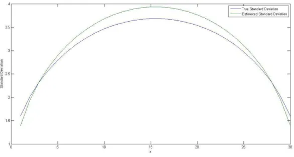
As can be observed in figures 3.1 and 3.2 the intuitive approximation suggested by variance proportional to distance to extremes is very precise(figure 3.1 has bothN(ρr, σ′2) andρ(x, y) overlapped),N(ρr, σ′2) andρ(x, y) are almost indistin-guishable in most points. The resemblance increases as the number of pointsnp, nq
increase although close to the edges (1,1) & (np, nq) the approximation continues
rough. The standard deviation also presents a satisfactory approximation and is also better the greaternp&nq are. The results depicted in figures 3.1 to 3.3 resemble
the consequences of the Central Limit Theorem just as the hypothesis of the set of functions resemble the hypothesis adopted by the theorem.
The approximation given by a variance proportional to distance can be extended toℜn(for optimization) and to problems where the construction of a statistical
Figure 3.4 displays the set of curves given bys1(x) with zero varying from 1
to 30. As demonstrated by the constructed theory, evaluating Step 1 of the generic root searching algorithm at the maximum ofs1(x) will yield maximum discard. An
example of how to use figure 3.4 is: Suppose an instance has zeroz= 4, by using figure 3.4 it is possible to identify the fourth curve (from the left to the right) and verify the maximum point of the curves1(x) to evaluate step 1 with maximum
average discard. Another use of figure 3.4 is to evaluate the statistical performance of a given strategy; to evaluate the bisection method, for example, the fourth curve evaluated at x1/2 will give the average discard operation of the this method for
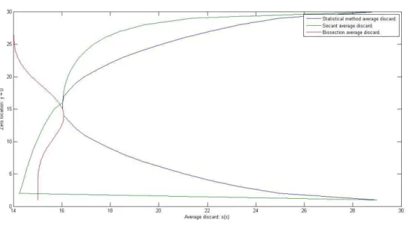
z= 4. Figure 3.5 has the performance of each of the three evaluated strategies with zero varying from 1 to 30.
The statistical performance of each strategy depicted in figure 3.5 shows the statistical superiority of the statistical method. When z = 15 the three strategies coincide and therefore have an optimal discard. Figure 3.5 also shows the lack of symmetry of the average discard of the bisection method and the secant method. This lack of symmetry observed is probably explained by the non-symmetry of the set of non decreasing functions; for the graphic of a function admits horizontal lines, but not vertical lines; and probably the effects of integer approximations also interfere in the results, especially of the secant method. A symmetric performance is expected to be observed over the set of strictly increasing methods (ρ(x, y) can be easily constructed for this set with very similar arguments used in this chapter). Figures 3.6 and 3.7 bring quite interesting insights. The first shows how each strategy selects x in Step 1 for zero varying from 1 to 30. In fact the curve that represents the statistical method in figure 3.6 illustrates what can be used as an abacus pre-calculated to follow a statistically optimal sequence of steps in the root bracketing strategy. What isn’t clear in the figure is that the statistical method tends to a smooth curve when the number ofnp&nqgrow, the indentations in its curve is
partly due to numerical approximations that are still rough withnp= 30 &nq= 30.
As discussed previously, a Pareto Optimal set of strategies is defined between the bisection method and the statistical method in each step, therefore evaluating last step situations figure 3.6 shows that the secant method is not Pareto Optimal. Figure 3.7 on the other hand shows that although in a two step evaluation ¯x26= ¯x1,
the average discard obtained by evaluating twice over maximum ofs1(x) will result
in almost maximum efficiency.
Another information contained in figure 3.7 is that ¯x2 is closer to the secant
method than ¯x1. Intuitively (although far from proven) it is possible to say that
although the secant method isn’t Pareto Optimal the statistical method does seem to converge to it when the number of steps n grows in a similar way that the statistical method converges to the the secant method whennp&nq→ ∞(this was
discussed at the end of section 3.2.1). If the statistical method indeed converges to the secant method for discrete non decreasing functions then a strong analogy can be done to the Fibonacci Method as it converges to the Golden Section Method in unidimensional optimization (this will be discussed in the next chapter).
This experiment shows that with a small list of tables it is possible implement with little computational effort optimal steps in root-searching. This can be of in-terest of mathematical programming platforms and of built-in routines of various software’s that crave for computational efficiency. Even the explicit calculation of s1ors2are, as shown by the experiment, computationally viable and therefore the
Optimal Maximum Searching
“It is the glory of God to conceal a matter; to search out a matter is the glory of kings.” Pv 25:2 NIV
Maximum Search
Maximum/minimum search or non-linear optimization algorithms are interactive sequential methods constructed to solve the following problem:
Maximization Problem. Given f : ℜn → ℜ a black-box function. Maximize:
f(x)Subject togi(x)≤0and tohj(x) = 0|i= 1, ..., ng andj= 1, ..., nh.
In optimization, functionf is called the objective function. A minimum of hypoth-esis is commonly assumed over the black-box functionf. In optimization, the sense of “best” strategy to solve a maximization problem is, as in other black-box se-quential searching problems, understood as those that simultaneously minimize at a maximum rate the possible location of the solution with a minimum amount of evaluations of the objective function. The reader will soon notice the close relation there is between root-searching and maximum-searching methods due to this same nature of black-box sequential searching.
Line Search
Line Search strategies, have served as a backbone to various optimization methods [8]. These strategies are divided into two main steps.
1. Choose from a starting point a descent direction, defining liner. 2. Maximize functionfover liner.
This second step of the Line Search methods is a unidimensional sub-problem known as unidimensional search. Thus unidimensional optimization strategies are of great importance in the optimization of multidimensional problems.
in these three decades. These unidimensional methods, with minor modifications, have remained as the main tools in modern optimization algorithms.
Fibonacci’s method, as well as the Golden Section method, stand for presenting a guarantee of a predictable convergence rate that does not depend on the nature of the objective function. As demonstrated by Kiefer [3] these methods are mini-maximal; this minimaximality can be comprehended as being optimal in a worst case situation, in a sense similar to what the bisection method is in root-searching. Parallel to this list of Line Search methods are the limited step methods such as the Trust Region methods [9, 2]. These methods may be identified as descendants of Levenberg-Marquardt algorithms that arose at the end of the 70’s and have produced a great amount of literature till present date. Although the increasing importance of these Trust Region methods, because it is a limited step method and doesn’t necessarily use concepts of discard and bracketing, these escape the scope of this work.
4.1 Classical Unidimensional Optimization
Now the unidimensional optimization problem and the classic non-randomized se-quential maximum-finding algorithm with a bracketing strategy will be presented:
Unidimensional Maximization Problem. Let f : [a, b] → ℜ be a black-box function. Givena, bandc∈(a, b)andya=f(a), yb=f(b), yc=f(c)withyc>(ya
&yb). Findx∗that maximizes:f(x)
Without loss of generality f may be assumed to be limited, for if f isn’t, it is possible to constructf′= tan−1◦f, and Im(f′)⊂[−π
2,
π
2] is limited and ifx∗
maxi-mizesfthen it maximizesf′as well. Functionfis usually assumed to be uni-modal or continuous. Either way the existence of a solution is guaranteed, in the first case by definition and in the second case by Weierstrass Theorem.
The classic non-randomized sequential maximum-finding algorithm with a brack-eting strategy is:
1. Chosex∈(a, b)|x6=c 2. Evaluatef(x)
3. If f(x)> yc andx > cmakea←candc←x
else iff(x)> yc andx < cmakeb←candc←x
else iff(x)< yc andx > cmakeb←x
else iff(x)< yc andx < cmakea←x
else iff(x) =yc then→ ∗1
4. If stopping criteria is met, return{a, ya, b, yb, c, yc}and stop.
Else go to step 1.
1 Different hypothesis over functionfredound in different actions over the finding
of f(x) =yc. In the case of f being uni-modal with strictly increasing function
It is imperative to say that many unidimensional optimization problems don’t start witha, b, c, ya, ybandycvalues and in this case, the algorithm starts by choosing
adequate values inf’s domain to evaluate and assign the respectivea, b, c, ya, yband
ycvalues.
As in root-searching algorithms different strategies vary mostly in how to chose x ∈ [a, b] and as can be imagined, interpolation is commonly used to predict the location of the maximum. Probably the most popular unidimensional maximization strategy is the Golden Section method. The Golden Section method is a particular case of the Fibonacci Sequence Method that is explained bellow:
4.1.1 Fibonacci Sequence Method (S∗
n)
LetUi be the i’th Fibonacci number given by:
U0= 0;U1= 1;Ui=Ui−1+Ui−2|i≥2
And letφ+i andφ−i be defined by: φ+
i =Ui/Ui+1 & φ−i =Ui−1/Ui+1|i >2
φ+2 =ǫ+U2/U2+1=ǫ+21 & φ−2 =U2−1/U2+1= 12
The Fibonacci Sequence methodS∗
n withnsteps supposes a starting condition
of having only values ofaandband is defined by: Starting withi←n
1. Calculatec=a+ (b−a)φ+i andx=a+ (b−a)φ−i
2. Execute steps 2-3 from the classic non-randomized sequential maximum-finding algorithm with a bracketing strategy.2
3. Ifi >2 updatei←(i−1) and go to step 1. Else return{a, ya, b, yb, c, yc}and end.
As the reader may notice, although step 1 of the Fibonacci Sequence method calculatescandx, it only needs to evaluatecandxat the first iteration, where at the subsequent, the values of either corxare already known due to the following property:
φ+i ×φ+i−1=
Ui
Ui+1×
Ui−1
Ui
=Ui−1 Ui+1
=φ−i
The Golden SectionS∗
∞ method is nothing more than the Fibonacci Sequence MethodSn∗defined by:
S∞∗ ≡ lim
n→∞S ∗
n
At each step ofS∗
nthe value ofφ+i andφ−i must be updated, whereas S∞∗ uses the fixed value given by:
φ= lim
n→∞φ
+
n =
√ 5−1
2 = 0,6180339887498948...
2 If step 2 is being executed for the first time it is necessary to evaluate function
&
φ−1= 1−φ=3− √
5
2 = 0,3819660112501052...
These two methods introduced by J.Kiefer [3] are mini-maximal over the set of the uni-modal functions with a maximum atx∗and strictly increasing from [a, x∗) and strictly decreasing from (x∗, b]. More precisely, Kiefer’s methods are, in his nomenclature:
Theorem 5.Given anyǫ >0and∀n= 1, ...,∞:
sup
f∈F
L(D(f, Sn∗))≤ inf S∈Snfsup
∈F
L(D(f, S)) +ǫ
D: set of all closed intervals within [a,b]. D∈D: Terminal decision.
n∈N: An integer.
Letgk: [a, b]k+1× ℜk+1→[a, b] be functions|k= 1, ..., n.
Ands &t: [a, b]n+2× ℜn+2→[a, b] : be functions|s≤t.
A strategySn, will be the setSn={a, b, ya, yb, g1, ..., gn, s, t}that can be computed
sequentially as the root searching algorithms:
xk=gk(a, b, x1, ..., xk−1, ya, yb, f(x1), ..., f(xk−1))|k= 1, ..., n
D(f, S) = [s(a, b, x1, ..., xn, ya, yb, f(x1), ..., f(xn)),
t(a, b, x1, ..., xn, ya, yb, f(x1), ..., f(xn))]
WithSnthe set of strategies{S|x∗∈D(f, S)∀f∈F whereF is the set of non
decreasingC0 functions.}andLis the length function.
A full demonstration of this result is presented in J.Kiefer’s [3] works.
4.1.2 Modified Bisection Method
Some modifications to the Bisection method where proposed for use in optimization, all of which, to the authors knowledge, have a performance necessarily worse than the Golden Section [4]. The variations of the modified bisection method seem to be preserved by literature in order exclusively to show superiority of the Golden Section method.
In this section an original modification to the Bisection method shall be pre-sented. This variation presents a superior performance in sets of functions with particular characteristics as will be shown. This method’s starting condition sup-poses thata, b, c, ya, ybandycare known, and if not, these values must be calculated
to begin the following algorithm:
Ifc= (a+b)/2 then go to step 1 - A. Else go to step 1 - B.
1. If ya≥ybcalculatex= (a+c)/2
Else ifya< ybcalculatex= (c+b)/2
2. Execute steps 2-3 from the classic non-randomized sequential maximum-finding algorithm with a bracketing strategy.
3. If stopping criteria is met, return{a, ya, b, yb, c, yc}and end.
Else ifc= (a+b)/2 then go to step 1 - A. Else go to step 1 - B.
Modified Bisection Method - Instance B
1. If k(c−a)k ≥ k(b−c)kcalculatex= (a+c)/2 Else ifk(c−a)k<k(b−c)kcalculatex= (c+b)/2
2. Execute steps 2-3 from the classic non-randomized sequential maximum-finding algorithm with a bracketing strategy.
3. If stopping criteria is met, return{a, ya, b, yb, c, yc}and end.
Else ifc= (a+b)/2 then go to step 1 - A. Else go to step 1 - B.
If the algorithm is initiated in instance A then the following iterations will nec-essarily either return to instance A or execute one iteration of instance B and return necessarily to A at the following iteration; this cycle will be called a steady state regime. If the algorithm starts at instance B withc6=a+1
3(b−a) andc6=a+ 2 3(b−a),
then the algorithm will run sequentiallynt times in instance B until its first
itera-tion in instance A, and from then on the algorithm will follow a steady state regime. Before the steady state regime is reached the cycle of nt iterations at instance B
will be called the transient regime.
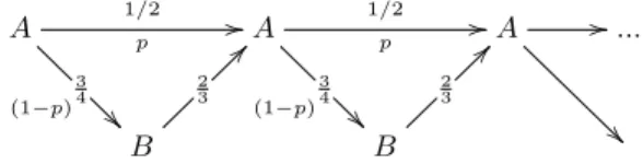
The resulting convergence rate of this version of the modified Bisection method can be studied by a diagram in which each arrow represents an evaluation of the objective function and its respective discard operation. The number above each ar-row is the convergence rate given by the discard operation and the number below represents the value of the probabilitypor (1−p) of this operations occurrence. For simplicity probabilitypwill be considered constant; this assumption is a scale invari-ance assumption that makes viable the analysis of the performinvari-ance of the modified bisection method. The upper row represents instance A and the lower one instance B.
Diagram 1 - Bisection Steady State Regime
A 3 4
(1−p)
1/2
p //A
3 4
(1−p)
1/2
p //A //...
B 2 3
?
?
B 2 3
?
Diagram 2 - Bisection Transient Regime A... A... B v1 p1 = = 1−v 1 2
1−p1
/ /B v2 p2 = = 1−v 2 2
1−p2
/
/
Modified Bisection Convergence Rate
The above diagrams serves of aid to calculate the convergence rate of the modified Bisection method during the steady state regime based on probability p. A more thorough analysis may be done including a similar convergence rate calculus with the transient regime although the reader may notice that in cases where the initial conditions don’t givecandyc, they may be chosen as to start the algorithm in the
steady state regime, being in this case, the analysis complete:
Theorem 6.Givenp, the probability at which the bisection method enters instance A from instance A, the value of the average convergence rate of the modified bisection method is given by:
r1 2 = 1 2 2−p1
Proof. The average convergence rate of a strategySn∈Snis defined as the number
r∈ ℜ |the new length of the region [a, b] afterniterations is equal torn×(b−a) =
(b−a)−sn .
This way, supposing the algorithm executedn iterations over instance A, then p×ntimes it whet directly from instance A to instance A and (1−p)×ntimes it went through instance B before. This results in the convergence rate given by:
r1 2 = " 1 2 p × 3 4
1−p
×
2 3
1−p#p×1+(1−p)×21
= " 1 2 p × 1 2
1−p#p+2−2p1
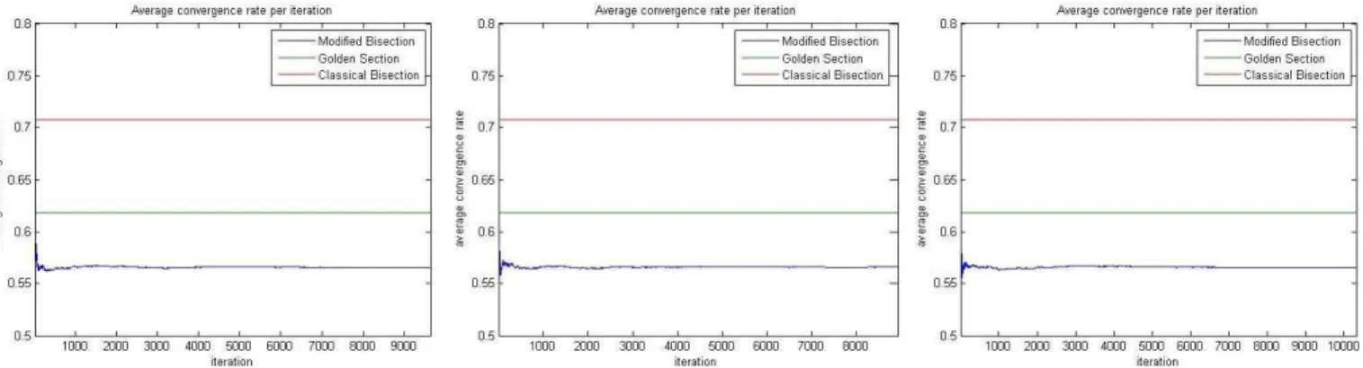
= 1 2 2−p1 ⊓ ⊔
The convergence rate of the Golden Section method is ofφ = (√5−1)/2 = 0.6180...so for any set of functions with p≥2 + logφ(2) = 0.5596...the Modified Bisection method will have in average a faster convergence rater1
2 =
1 2
2−p1
Given a setFof functions,f∈Fa function chosen at random and evaluated at three pointsa, bandcwithc= (a+b)/2, and supposing without loss of generality that f(b) > f(a). Then p is the probability that function f has function value y(x)> y(c) atx= (b+c)/2.
This “inertia” condition is perfectly possible in sets of functions thatxfunction values carry information of the location of neighbour values such as in differentiable functions. Function sets that have tendency to have maximum at extremes will also be favoured by this method over the Golden Section method.3
Sub-Optimality of the Modified Bisection Method
As discussed in the previous section, the Fibonacci sequence is a mini-maximal algorithm with a starting condition in which c and yc isn’t given over the set of
uni-modal functions. One may ask how to obtain a method that is mini-maximal over the same set of functions but with a starting condition in whicha, bandcand ya, ybandycare given.
At first all mini-maximal strategiesS1 ∈S1 with givena, b, c, ya, yb andyc will
be analysed. As usual the following assumptions are made:yc> ya andyc> yb.
As in root searching mini-maximal strategies “minimize” 4 objective function
Ondefined by:
On:Sn→ ℜ |On(Sn) = sup f∈F
L(D(f, S))
Ifc > 12(a+b) it is easy to perceive that any strategy S1 ∈ S1 that evaluates
x∈[a+b−c, c) is then mini-maximal. Ifc < 1
2(a+b) the argument is analogous,
but ifc= 1
2(a+b) then the Fibonacci Sequence strategyS∗1 is the “minimizer” of
On. It is possible to notice thatS1that minimizesO1isn’t unique, this is also true forOnand the number of “minimizers” ofOnare infinite∀n∈N.
Considering once more the case whenc > 1
2(a+b), the set of minimizing
strate-gies of O1 can evaluate a randomly selected function f and execute the discard operation over either [a, x] or [c, b]. The second possibility is the same for all mini-mizers, but evidentlyl[a, x] varies withxand can be chosen to beδmaximum, this is achieved with x =c−δ. A first version of the bisection method for optimiza-tion(that is not the case of the presented method) executes consecutive evaluations of the objective function overc= (a+b)/2 andx=c−δwhich is to say very similar to what could be called a reinitialization of aS1method withδmaximum possible discard operations.
What is interesting about the presented modified bisection method is that it is easy to demonstrate that at every step it evaluates the objective function f at x given byS2that “minimizes”O2. This way while the classical bisection method for 3 The reader may verify that some subsets of the polynomials have such “inertia”.
As an example of such subsets the author suggests a numerical verification of the Modified Bisection method between the first two roots of randomly generated tenth degree polynomials P(x) = Pc
ixi by uniformly generating coefficients
ci∈[−1,1]|i= 1, ...,9 andc0∈[0,1] andc10∈[−1,0].
4 “minimize” is between quotation marks because as in Kiefer’s demonstrated
sit-uation, there isn’t a minimizer in strict sense. Kiefer’s theorem guarantees that ∃S∗|sup
f∈FL(D(f, Sn∗))≤infS∈Snsupf
optimization is a reinitialization of a strategyS1 that minimizesO1, the modified bisection method is a reinitialization of aS2 that minimizesO2.
Exercise 6. Find the set of strategies that minimize O3 with given initial values ofa, b, c, ya, ybandyc . (Hint: What isS3∗?)
For a better illustration on the modified bisection performance a numerical ex-periment shall be constructed at the end of this chapter to compare the efficiency of this method with the efficiency of the golden section method.
4.2 Statistical Performance
4.2.1 Statistical Optimization Method
Statistical Optimization is very similar to Statistical Root searching. As discussed in the Statistical Performance section of root searching methods, to obtain a sta-tistically optimal convergence over a determined set of functionFit is necessary to construct a Statistical Characterization of the set of functions being investigated.
In root search two main theorems where demonstrated to obtain the charac-terization of different sets of functions. Theorem 2 gives the means to characterize sets of functions F ={fq(x) = g(q, x) | q ∈ [0,1]p ⊂ ℜp} while Theorem 3 gives
the characterization of the set of discrete non decreasing functions. In both Opti-mization and in Root Search Theorem 2 can be used for any set of functions that may be described by parametersq ∈ ℜn. On the other hand Theorem 3 has little
value in optimization, since non decreasing functions have a pre-determined loca-tion of the maximum. For optimizaloca-tion it is of more interest the characterizaloca-tion of uni-modal functions with constraints of f(a) =ya, f(b) =yb and f(c) =yc since
the Fibonacci sequence is mini-maximal over this set, and at each step of the clas-sical non-randomized bracketing strategy ya, yb and yc are known. This way the
performance of these two methods can be compared.
To construct the characterization of uni-modal functions the following lemma will be necessary:
Lemma 5.The number of (strictly) increasing functions from A = {1, ..., np} to
B={1, ..., nq}withnq≥npis given by :
#f
~ w w w
{1,...,nq} {1,...,np}
= #solutions{c1+c2+...+cnp+1=nq−np|ci∈N∗}=
nq!
(nq−np)!np!
Proof. Given a solution functionf, without loss of generality it is possible to consider thatf(0) = 0 andf(np+ 1) =nq+ 1. Letc∗i =f(i)−f(i−1)|i= 1, ..., np+ 1, so
c∗
1+c∗2+...+cn∗p+1=nq+1 for each increasing functionfandc ∗
i ∈Nforfis strictly
increasing. Defineci=c∗i −1, thereforec1+c2+...+cnp+1=nq−npandci∈N∗
this implies that for each increasing functionfdefined from{1, ..., np}to{1, ..., nq}
there is a unique set of values forcisatisfyingc1+c2+...+cnp+1=nq−np, and for each solution toc1+c2+...+cnp+1=nq−np|ci∈N∗there is a unique increasing function defined from{1, ..., np}to{1, ..., nq}.
Therefore the first equality of the Lemma yields.