ELIMINATION OF SOME UNKNOWN PARAMETERS AND
ITS EFFECT ON OUTLIER DETECTION
Eliminação de alguns parâmetrtos desconhecidos e seu efeito na detecção de erros grosseiros
SERIF HEKIMOGLU1 BAHATTIN ERDOGAN1 NURSU TUNALIOGLU1
1
Yildiz Technical University Faculty of Civil Engineering Department of Geomatic Engineering
Davutpasa Campus, 34220 - Esenler- Istanbul, Turkey [email protected]; [email protected]; [email protected]
ABSTRACT
Outliers in observation set badly affect all the estimated unknown parameters and residuals, that is because outlier detection has a great importance for reliable estimation results. Tests for outliers (e.g. Baarda’s and Pope’s tests) are frequently used to detect outliers in geodetic applications. In order to reduce the computational time, sometimes elimination of some unknown parameters, which are not of interest, is performed. In this case, although the estimated unknown parameters and residuals do not change, the cofactor matrix of the residuals and the redundancies of the observations change. In this study, the effects of the elimination of the unknown parameters on tests for outliers have been investigated. We have proved that the redundancies in initial functional model (IFM) are smaller than the ones in reduced functional model (RFM) where elimination is performed. To show this situation, a horizontal control network was simulated and then many experiences were performed. According to simulation results, tests for outlier in IFM are more reliable than the ones in RFM.
Keywords: Elimination; Tests for Outliers; Reliability; Adjustment.
RESUMO
testes de Baarda e Pope) são utilizados frequentemente na detecção de erros grosseiros em aplicações geodésicas. Muitas vezes, visando reduzir o tempo computacional, é realizada a eliminação de alguns parâmetros que não são de interesse. Nesse caso, embora a estimativa dos parâmetros e resíduos não sofra modificações, a matriz cofatora dos resíduos e a redundância das observações mudam. Nesse estudo, são realizados testes para erros grosseiros e investigados os efeitos da eliminação dos parâmetros desconhecidos. Foi provado que quando a eliminação é realizada, as redundâncias no modelo funcional inicial (IFM – Initial Functional Model) são menores que no modelo funcional reduzido (RFM – Reduced Functional Model). Para ilustrar essa situação, uma rede de controle horizontal foi simulada e muitos experimentos foram realizados. De acordo com os resultados da simulação, testes para erros grosseiros com IFM são mais confiáveis que com RFM.
Palavras-chave: Eliminação; Testes para Erros Grosseiros; Confiabilidade; Ajustamento.
1. INTRODUCTION
Outlier detection has a great importance in geodetic networks. The efficacy of the unknown parameters and their standard deviations depends on whether the observation set includes outliers or not. Sometimes, observations may contain one or more outliers. In this case, these outliers must be detected and removed or re-measured. Tests for outliers are mostly used for the outlier detection (BAARDA, 1968; POPE, 1976; KOCH, 1999). The efficacies of the tests for outliers change depending on the number of outliers and the magnitudes of outliers (HEKIMOGLU and KOCH, 2000). Tests for outliers can detect only one outlier reliably (HEKIMOGLU, 1997; BASELGA, 2007; HEKIMOGLU et al., 2011). If the observations include more than one outlier, the tests for outliers cannot detect them reliably due to masking effect or swamping effect, especially when the magnitudes of multiple outliers are small (HEKIMOGLU, 2000 and 2005).
To apply outlier detection, the observations of the geodetic networks are adjusted as a free network. First, the unknown parameters, which are not related to the coordinates of the points, are eliminated to interpret the unconstrained adjustment model geometrically (NIEMEIER, 2002). A similar problem to eliminate the orientation parameters is commonly occurred in triangulation networks. Some unknown parameters that are not of interest are generally eliminated. In this context, two different functional models come up: (1) the initial functional model (IFM) and (2) the reduced functional model (RFM), where elimination is performed.
Although the estimated unknown parameters and residuals in RFM are the same as the ones in IFM, the cofactor matrix of residuals and redundancies ri of the observations are different. In this study, firstly, we figure out this situation. Secondly, we investigate whether the differences among the redundancies may affect the outlier detection or not. Also, the following question is investigated: must the outlier detection be applied to RFM or IFM where a group of unknowns is not eliminated?To compare the reliabilities of tests for outliers in RFM and IFM, mean success rate (MSR) is used. The MSR was introduced to measure the efficacy of the tests for outliers (HEKIMOGLU and KOCH, 2000). The MSR is globally the number of successful detections over the number of experiments. The MSR also means the estimated power of the test (AYDIN, 2011).
2. ELIMINATION BY PARTITIONING BLOCKS
A general approach for eliminating some (or a group) unknown parameters is to split the functional model into blocks. The linearized IFM is given as follows:
, (1) where l is the observation vector, v is the residual vector, A is the coefficient (design) matrix of the unknown parameters, x is the unknown vector, is the variance of unit weight, P is the diagonal weight matrix, is the cofactor matrix of the observations and is the variance covariance matrix of the observations. Then the design matrix and the unknown vector given in Eq. (1) are divided into two sub-matrices and sub-vectors:
, (2) where the sizes of A1, A2, x1 and x2are n x p, n x q, p x 1 and q x 1, respectively. X1
contains the main unknown parameters, x2 also contains the unknown parameters,
which are eliminated. N is the number of observations, p is the number of main unknown parameters and q is the number of eliminated unknown parameters. In this case, Eq. (1) can be written as follows:
(4)
(5)
(6)
Here, if is invertible, in the Eq. (4) x2 can be written as a function of x1:
(7) If Eq. (7) is put in the first equation of the Eq. (4),
(8) Eq. (8) can be written shortly,
(9) Eq. (10) is obtained for the inverse of the ,
(10) In this way, the solution of the vector x1for RFM can be obtained from Eq.
(9):
(11) As calculating the block matrices in IFM, the sub-matrices of the cofactor matrix Q are determined. To obtain the sub-matrices, the following equations are usually used:
(12)
where E denotes the identity matrix. If the sub-matrix N22 is regular, i.e. it is
invertible; the following equations can be obtained as (Faddejew and Faddejewa, 1976):
(13)
(14) Also, if Eq. (14) is considered in Eq. (12):
(15) The above equation can be obtained, by taking advantage of the symmetry property, the following equation can be written as follows:
(16) If Eq. (10) and Eq. (15) are compared to each other, it can be seen that the cofactor matrix of the x1 is equal to the cofactor matrix Q11 in IFM, i.e.
. Elimination does not change the cofactor matrix.
To determine the unknown vector x2in RFM, x1is obtained from Eq. (11) and
put into Eq. (7). It is important to determine the residuals in RFM. If x2 is obtained
from Eq. (7) and put into Eq. (3), the residuals can be computed as follows:
(17) If the terms of this equation are shortened as follows:
(19) (20) Eq. (18) can be written differently:
(21) There will not be any change for the estimation value of the variance .
(22) The equations in this section can be adapted to free network adjustment (HECK, 1975).
3. COMPARING THE REDUNDANCIES OF THE OBSERVATIONS IN RFM WITH THE ONES IN IFM
The H and R matrices in IFM are given as follows:
(23)
(24)
where H denotes the hat matrix in statistics and matrix can be written from Eq.
(4) as and the hat matrix can be written from Eq. (23) as
below.
(25)
(26) If Eq. (13) and Eq. (14) are considered, the following Eq. can be obtained:
(27) Since the symmetry property, , Eq. (27) can be rewritten as below:
(28) If Eq. (16) is considered in Eq. (28), Eq. (29) can be obtained:
(29) Since;
H can be rewritten as follows:
P (30)
For RFM, the following two equations from the Eq. (18) can be written: (31)
Since , , and
, Eq. (31) can be written as below:
(33)
(34)
(35) If Eq. (30) and (35) are taken into account, Eq. (36) can be obtained:
(36) Since is a quadratic form, it can be expressed as
. Therefore is always bigger than h , i.e. h h and
also , since and .
The equations in this section can be adapted to free network adjustment (HECK, 1975).
4. TESTS FOR OUTLIERS
Outlier detection procedures were proposed by Baarda (1968) and Pope (1976) for geodesy. In these outlier detection processes, “good” observations originate from the same distribution, which is generally expressed as a normal distribution
, . Observations that contain outliers are called as “bad” observations. Let an observation l′′ has an outlier δl with l′′ l′ δl. The hypothesis
H : δl against H : δl is tested. If the observations are uncorrelated and the variance σ is known, the standardized residuals derived from IFM can be presented as:
| |
(37ª)
where is the diagonal elements of .
If ⁄ , which is the upper ⁄ percentage point of the normal distribution, the observation ′′ is accepted as a bad observation where α is chosen as 0.001. This is called as Baarda’s method. If there is more than one outlier among the observations, Baarda’s method is used iteratively (BAARDA, 1968).
If the variance is not known before, the studentized residual is used for Pope’s test:
| |
(37b)
where is given in Eq. (22). If the level of significance α is related to all observations, the level of each observation must be ⁄ . , ,
⁄ where , , ⁄ , , .
If the following relations are taken into account,
(39)
(40) the below relation can be written as:
(41)
If the Eqs. (37a) and (37b) are rewritten by considering Eq. (41), the following equations can be obtained
| |
(42ª)
| |
(42b)
If rank A=q holds in the Gauss-Markov model, then
, , ⁄ , , , where α is generally chosen as 0.05 or 0.01 (Koch,
1999).
For RFM, we can generate the following equations similar to Eqs. (39) and (40).
(43)
(44) If above two equations are considered, the following equation can be written as
(45)
and similar to Eqs. (42a) and (42b), the followings can be obtained: | |
(46ª)
| |
(46b)
Since , and in IFM are bigger than and in RFM, respectively. It means that the effects of the outlier with small magnitude in IFM may be reflected stronger than the ones in RFM on the standardized or studentized residuals. Therefore, the MSRs of the tests for outliers in IFM become bigger than the MSRs of the ones in RFM.
5. CASE STUDIES
5.1 Elimination of orientation parameters in triangulation network
The method dating back to C. F. Gauss uses the elimination of the orientation parameters at triangulation networks. If we consider only one unknown parameter, which has the same coefficient in the residual equations, it can be regarded as a special case of the elimination. For elimination of the only one unknown x2(q=1 in
Eq. (2)), the related design matrix can be written:
, T … , T
where the size of the A2is nx1 and k is the number of direction observations at one
station. If P = I, the reduced approach according to Eq. (19) is given as follows:
(48)
(49)
where means column sum of the A1 (it must be multiply by 1/k) (Niemeier,
2002). At the same time, it should be eliminated from the initial residual equations. is obtained similarly,
(50)
(51)
where column sum of is similarly divided by k and reduced from li. Mean residual equation that is eliminated from each residual equation is computed as follows:
(52) In practice, Eq. (52) is computed for each station by which direction observations are made at the network. The linearized residual equations for a station, in which k direction measurements are made can be written with the orientation parameter o:
(53)
Reduced residual equations are obtained as follows:
(54)
where ∑ , ∑ , ∑
5.2 Simulation
In this study, a Monte-Carlo simulation technique has been used to demonstrate as above described case. To measure the reliability of tests for outliers in IFM and RFM, a horizontal control network was simulated. Fig. 1 presents the positions of the points and observations for the horizontal control. The simulated horizontal control network given in Figure 1 consists of 7 points where n = 48, u = 21 and degrees of freedom f = 30. The MSRs for IFM and RFM are presented for the same network. All results have been obtained using MATLAB version R2006a.
are obtained as the same as Hekimoglu and Erenoglu (2007), Erenoglu and Hekimoglu (2010), Hekimoglu et al. (2011).
For the horizontal control network, the observations, such as direction measurements and distance measurements are computed from the coordinates of the points. They are free of random errors. The random errors are generated from a normal distribution as follows: for direction measurements ~ , with
mgon and for the distance measurements ~ , with
where Sij is the distance between ith and jth points. The random errors are added to the distance and direction measurements such as ′ and ′ . Hereby, the good observations are obtained.
Then, the random error is replaced by the outlier in the related observation as ′′ ′ , thus the contaminated observations ′′ are obtained. The approximate
values of the point coordinates are given in Table 1. The direction measurements and distance measurements are also given Table 2 and Table 3, respectively.
Figure 1 – Simulated horizontal control network.
Table 1 – The approximate values of the points’ coordinates shown in Fig. 1.
Y (m) X (m)
1 -45162.050 4405916.380 2 -42162.060 4405916.376
3 -39162.681 4405916.459 4 -43565.155 4403318.288 5 -40565.774 4403318.360 6 -44824.810 4408514.459
Table 2 – The direction measurements and standard deviations.
Observation Number
Directions From to
Observed values
(gon)
Standard Deviations
(mgon)
1 1 6 20.0004 0.3
2 7 69.6757 0.3
3 2 111.7825 0.3
4 5 144.5358 0.3
5 4 176.6981 0.3
6 2 7 19.9987 0.3
7 3 111.7675 0.3
8 5 176.6938 0.3
9 4 243.2922 0.3
10 1 311.7673 0.3
11 6 360.9849 0.3
12 3 5 20.0002 0.3
13 4 54.5348 0.3
14 2 88.4752 0.3
15 7 137.7074 0.3
16 4 2 20.0008 0.3
17 3 54.5355 0.3
18 5 88.4755 0.3
19 1 353.3907 0.3
20 6 373.3349 0.3
21 5 3 20.0003 0.3
22 4 288.4753 0.3
23 1 321.2286 0.3
24 2 353.4017 0.3
25 6 7 19.9992 0.3
26 2 69.2171 0.3
27 4 104.8596 0.3
28 1 128.2172 0.3
29 7 3 20.0001 0.3
30 2 79.0007 0.3
31 1 128.6606 0.3
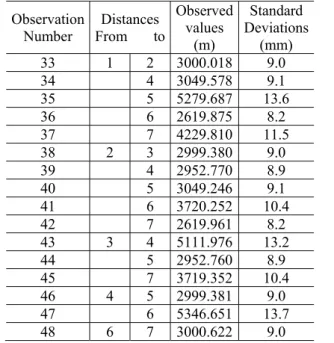
Table 3 – The distance measurements and standard deviations.
Observation Number
Distances From to
Observed values
(m)
Standard Deviations
(mm)
33 1 2 3000.018 9.0
34 4 3049.578 9.1
35 5 5279.687 13.6
36 6 2619.875 8.2
37 7 4229.810 11.5
38 2 3 2999.380 9.0
39 4 2952.770 8.9
40 5 3049.246 9.1
41 6 3720.252 10.4
42 7 2619.961 8.2
43 3 4 5111.976 13.2
44 5 2952.760 8.9
45 7 3719.352 10.4
46 4 5 2999.381 9.0
47 6 5346.651 13.7
48 6 7 3000.622 9.0
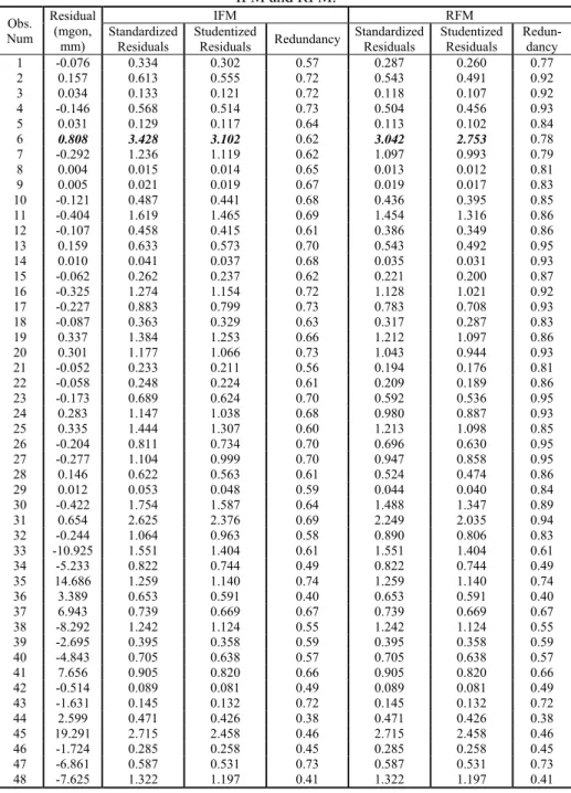
Table 4 - The redundancy, standardized and studentized residuals for IFM and RFM.
Obs. Num
Residual (mgon,
mm)
IFM RFM Standardized
Residuals
Studentized
Residuals Redundancy
Standardized Residuals
Studentized Residuals
Redun-dancy
1 -0.076 0.334 0.302 0.57 0.287 0.260 0.77
2 0.157 0.613 0.555 0.72 0.543 0.491 0.92
3 0.034 0.133 0.121 0.72 0.118 0.107 0.92
4 -0.146 0.568 0.514 0.73 0.504 0.456 0.93
5 0.031 0.129 0.117 0.64 0.113 0.102 0.84
6 0.808 3.428 3.102 0.62 3.042 2.753 0.78
7 -0.292 1.236 1.119 0.62 1.097 0.993 0.79
8 0.004 0.015 0.014 0.65 0.013 0.012 0.81
9 0.005 0.021 0.019 0.67 0.019 0.017 0.83
10 -0.121 0.487 0.441 0.68 0.436 0.395 0.85
11 -0.404 1.619 1.465 0.69 1.454 1.316 0.86
12 -0.107 0.458 0.415 0.61 0.386 0.349 0.86
13 0.159 0.633 0.573 0.70 0.543 0.492 0.95
14 0.010 0.041 0.037 0.68 0.035 0.031 0.93
15 -0.062 0.262 0.237 0.62 0.221 0.200 0.87
16 -0.325 1.274 1.154 0.72 1.128 1.021 0.92
17 -0.227 0.883 0.799 0.73 0.783 0.708 0.93
18 -0.087 0.363 0.329 0.63 0.317 0.287 0.83
19 0.337 1.384 1.253 0.66 1.212 1.097 0.86
20 0.301 1.177 1.066 0.73 1.043 0.944 0.93
21 -0.052 0.233 0.211 0.56 0.194 0.176 0.81
22 -0.058 0.248 0.224 0.61 0.209 0.189 0.86
23 -0.173 0.689 0.624 0.70 0.592 0.536 0.95
24 0.283 1.147 1.038 0.68 0.980 0.887 0.93
25 0.335 1.444 1.307 0.60 1.213 1.098 0.85
26 -0.204 0.811 0.734 0.70 0.696 0.630 0.95
27 -0.277 1.104 0.999 0.70 0.947 0.858 0.95
28 0.146 0.622 0.563 0.61 0.524 0.474 0.86
29 0.012 0.053 0.048 0.59 0.044 0.040 0.84
30 -0.422 1.754 1.587 0.64 1.488 1.347 0.89
31 0.654 2.625 2.376 0.69 2.249 2.035 0.94
32 -0.244 1.064 0.963 0.58 0.890 0.806 0.83
33 -10.925 1.551 1.404 0.61 1.551 1.404 0.61
34 -5.233 0.822 0.744 0.49 0.822 0.744 0.49
35 14.686 1.259 1.140 0.74 1.259 1.140 0.74
36 3.389 0.653 0.591 0.40 0.653 0.591 0.40
37 6.943 0.739 0.669 0.67 0.739 0.669 0.67
38 -8.292 1.242 1.124 0.55 1.242 1.124 0.55
39 -2.695 0.395 0.358 0.59 0.395 0.358 0.59
40 -4.843 0.705 0.638 0.57 0.705 0.638 0.57
41 7.656 0.905 0.820 0.66 0.905 0.820 0.66
42 -0.514 0.089 0.081 0.49 0.089 0.081 0.49
43 -1.631 0.145 0.132 0.72 0.145 0.132 0.72
44 2.599 0.471 0.426 0.38 0.471 0.426 0.38
45 19.291 2.715 2.458 0.46 2.715 2.458 0.46
46 -1.724 0.285 0.258 0.45 0.285 0.258 0.45
47 -6.861 0.587 0.531 0.73 0.587 0.531 0.73
To measure the reliabilities of the tests for outliers, the MSR criterion has been handled. A test for outlier is regarded as successful when the test statistics can separate the null hypothesis H0 from the alternative hypothesis H1 at the significance level α. The mean success rate (MSR) is defined with dividing the number of success by the number of experiments. If a good sample is contaminated by replacing any number of the observations with arbitrary values, then a contaminated sample obtained. Many good samples can be obtained by generating the different subsets of random errors. Thus, for each good sample, many contaminated samples are generated by replacing any number of good observations with arbitrary values.
Since a simulation is used to generate the outliers, it is possible to know exactly whether an observation is contaminated or not, in advance of carrying out the analysis. After applying the outlier detection method, if the observation is identified as an outlier and it corresponds to truly contaminated observation, the method is regarded as successful. If the method fails, it is considered unsuccessful (HEKIMOGLU and ERENOGLU 2007, HEKIMOGLU and KOCH 2000, ERENOGLU and HEKIMOGLU 2010, HEKIMOGLU et al. 2011). Owing to using simulation techniques, a lot of samples can be generated easily. The MSR is globally the number of successful detections over the number of experiments.
The magnitudes of the small outliers (whose magnitudes lie between and
6 ), and large outliers (whose magnitudes lie between 6 and ), are generated separately. Also, both tests for outliers are iteratively applied. Only the observation with the largest normalized or studentized residual is tested and in case it is rejected, it is removed and the remaining observations are then adjusted again. But, in this case, a geometric defect of the network may occur. To prevent such a geometric defect, the detected observation is not removed; instead of this, the related weight of the observation is set smaller for the next iteration step, for example pi=0.001 x
pi. In this case, the initial approximation of the orientation is estimated by using the weighted arithmetic mean.
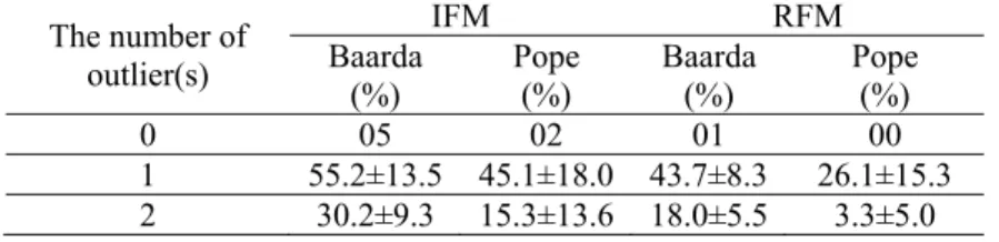
Table 5 – The MSRs of IFM and RFM for the magnitudes which lie between 3σ and 6σ.
The number of outlier(s)
IFM RFM Baarda
(%)
Pope (%)
Baarda (%)
Pope (%)
0 05 02 01 00
1 55.2±13.5 45.1±18.0 43.7±8.3 26.1±15.3
Table 6 – The MSRs of IFM and RFM for the magnitudes which lie between 6σ and 12σ.
The number of outlier(s)
IFM RFM Baarda
(%)
Pope (%)
Baarda (%)
Pope (%)
1 94.5±19.9 96.7±10.9 95.6±10.9 95.1±5.9
2 93.6±18.1 92.1±11.6 90.3±10.5 75.8±13.9
The orientation parameters are eliminated in RFM; whereas they are estimated in IFM. Also, the observations at the network given in Fig. 1 were adjusted as free network. Tables 5 and 6 include the MSRs of both Baarda’s and Pope’s tests for IFM and RFM. The MSRs are increased by 11.5% (55.2% - 43.7%) and 19.0% (45.1% - 26.1%) for the Baarda’s and Pope’s tests, respectively, for one small outlier. Also, the reliability of IFM for two outliers is bigger than the ones of RFM. However, the MSRs of IFM are bigger than the RFM when there is no outlier in observation set. This is the type I error. The increase in type I error for IFM is 4% (5% - 1%) for Baarda’s test and 2% (2% - 0%) for Pope’s test. The advantage of IFM is 7.5% (11.5% - 4%) for Baarda’s test and 17% (19% - 2%) for Pope’s test. However, for one large outlier the MSRs for both tests are not increased significantly.
6. CONCLUSION
Elimination of the unknown parameters in adjustment model is sometimes preferred to shorten the calculation time. Although the estimated unknown parameters, residuals, cofactor matrix of the unknown parameters in IFM are the same as the ones in RFM, the cofactor matrix of the residuals and redundancies of the observations are different. The redundancies in IFM are smaller than the ones in RFM; this situation is proved in this study. Since the diagonal elements of the cofactor matrix of the residuals in RFM is bigger than the ones in IFM, the standardized residuals or studentized residuals in IFM are bigger than RFM. Therefore, the effects of the outliers do not appear strongly on the residuals for some cases of RFM where the magnitude of outlier is small, and the outliers cannot be detected.
R A A B B E F G H H H H H H H H K K K M N REFERENC
ALBERTZ, J Karlsruhe AYDIN, C. O
doi:10.10 BAARDA, W
Geodesy, BASELGA, S
Eng. 133( ERENOGLU, outliers fo 439, 2010 FADDEJEW, Algebra, 4 GHILANI, C. edition, Jo HECK, B. Di
Ausgleich HEKIMOGLU outlier de HEKIMOGLU measured HEKIMOGLU
is Small. S
HEKIMOGLU conventio Jahrgang, HEKIMOGLU heterogen 81(2):137 HEKIMOGLU Increasing Geod. Ge
HÖPCKE, W 1980. KING, R. W.
with Glob KOCH, K. R.
Springer-V KRAUS, K. P MIKHAIL, E SeriesCiv NIEMEIER, W
ES
J.; KREILING e,1989. On the Power
61/(ASCE)SU W. A testing p New Series 2 S. Critical lim (2): 52–55, 20 , R. C.; HEKI or geodetic ad 0.
D. K.; FAD 4. Aufl., Mün .D.; WOLF, P ohn Wiley & ie Genauigkei hungsproblem U, S. The fini tection proced U, S.; KOCH d? Allg. Verme
U, S. Increasi
Surv. Rev., 38 U, S. Do r onal tests fo , Heft 3, 2005 U, S.; ERE neousness on 7-148, 2007.
U, S.; ERDO g the Efficacy
eoph. Hung., 4 W. Fehlerlehre ; MASTERS, bal Positioning Parameter es Verlag, Berlin Photogrammet E. M.; ACKE vil Engineering
W. Ausgleichu
G, W. Photog
r of Global Te U.1943-5428.0 procedure for 2, no.5, Nether mitation in use
007
IMOGLU, S. djustment mod
DDEJEWA, W nchen-Wien. R P. R. Adjustme Sons Inc., 200 it eliminierter men. Allg. Verm
ite sample bre dures. J. Surv.
H, K. R. Ho
ess. Nachr. 10 ing Reliability 8(298), 274-28 robust metho
r outliers? Z .
ENOGLU, R outlier dete
OGAN, B.; y of the Tests 46(3), 291-308 e und Ausgle
E. G.; RIZO g System GPS stimation and
n, 1999. try, Volume 2 ERMANN, F. g, New York, ungsrechnung
grammetric H
est in Deform 0000064, 201 r use in geode
rlands Geodet of test for
Efficiency of dels. Acta Ge
W. N. Numer R. Oldenbourg ent Computati 06.
r Unbekannter
mess. Nachr., eakdown point
. Eng.,123(1), ow can reliab 7/7: 247–254 y of the Test 85, 2005. ods identify
Zeitschrift fu
R. C. Effect ection for ge
ERENOGLU s for Outliers 8, 2011. eichsprobleme
S, C.; STOLZ S. Ferd. Dümm
hypothesis tes
2, 4th ed., Düm . E. Observat
1976. g, Walter de G
andbook, Her
mation Analys 1.
etic Networks tic Commissio gross error d
f robust meth
eod. Geoph. H
rische Metho g-Verlag, 1976
ions: Spatial D
r bei regulare 82,345-348, 1 ts of the conv 15-31, 1997. bility of tests
, 2000. for Outliers w
outliers mor uer Vermessu
t of heteros eodetic Netw
U, R. C.; H for Geodetic
e. Walter de
Z, A.; COLLIN mler Verlag, B
sting in linear
mmler, Bonn, tions and Le
Gruyter, Berlin
rbert Wichma
sis. J. Surv. E
s. Publication on, Delft, 196 detection. J. Su
hods and tests
Hung. 45(4):4
den der linea 6.
Data Analysis
n und singula 1975. ventional iterat
s for outliers
whose Magnit
re reliably t ungswesen, 1
scedasticity works. J. Ge
HOSBAS, R. c Networks. A
Gruyter, Ber
NS, J. Survey Bonn, 1987. r models. 2nd
1997. ast-Squares. n, 2002. ann, Eng. n on 8. urv. for 426-aren
, 4th
POPE, A J. The statistics of residuals and the outlier detection of outliers. NOAA Technical Report, NOS 65, NGS 1, Rockville, MD, 1976.
STRANG, G.; BORRE, K. Linear algebra, geodesy, and GPS. Wellesley-Cambridge Press, 1997.
WOLF, H. Ausgleichungsrechnung nach der Methode der kleinsten Quadrate. Dümmler, Bonn, 1968.