Partial least squares for face hashing

PARTIAL LEAST SQUARES

C ´

ASSIO ELIAS SANTOS J ´

UNIOR

PARTIAL LEAST SQUARES

FOR FACE HASHING

Disserta¸c˜ao apresentada ao Programa de P´os-Gradua¸c˜ao em Ciˆencia da Computa¸c˜ao do Instituto de Ciˆencias Exatas da Univer-sidade Federal de Minas Gerais como req-uisito parcial para a obten¸c˜ao do grau de Mestre em Ciˆencia da Computa¸c˜ao.

Orientador: William Robson Schwartz

C ´

ASSIO ELIAS SANTOS J ´

UNIOR

PARTIAL LEAST SQUARES

FOR FACE HASHING

Dissertation presented to the Graduate Program in Computer Science of the Uni-versidade Federal de Minas Gerais in par-tial fulfillment of the requirements for the degree of Master in Computer Science.

Advisor: William Robson Schwartz

©  2015, Cassio Elias dos Santos Junior

    Todos os direitos reservados

Ficha catalográfica elaborada pela Biblioteca do ICEx ­ UFMG

Santos Júnior, Cássio Elias.

S237p     Partial least square for face hashing / Cássio Elias          Santos Júnior. —  Belo  Horizonte, 2015.

    xxviii, 72f. : il. ; 29cm.

      Dissertação (mestrado) ­ Universidade Federal de        Minas Gerais Departamento de Ciência da             Computação.

       Orientador: William Robson Schwartz.

       1. Computação ­ Teses. 2.  Visão por computador­        Teses. 3 Indexação de imagens­ Teses  I. Orientador 

      II. Título.

Acknowledgments

First, I would like to thank deeply professor William Robson Schwartz for the out-standing orientation on my undergraduate and graduate studies.

I would also like to thank professors Ewa Kijak, Guillaume Gravier and Silvio J. F. Guimar˜aes for their intellectual and financial support without which this work would never be completed.

I thank the members of the examination committee, professors Erickson R. do Nascimento and Carlos E. Thomaz, for the enrichment that they brought to this work. I am eternally thankful for all support that my parents gave me, allowing me to focus on research and studies.

I am very grateful for my beloved Jessica I. C. Souza for all support and love that she gave me throughout my master.

I am also very grateful for all members of the SSIG team, the NPDI lab and the Linkmedia team for kindly receiving me in such amiable way and for all my friends in Brazil: Adriano F. Schiavon, Andrey Bicalho Santos, Antˆonio A. Nazar´e Jr., Artur J. L. Correia, Bruno do N. Teixeira, Carlos A. Caetano Jr., Carlos A. P. Filho, C´esar A. M. Ferreira, David Saldana, Elerson R. da S. Santos, Filipe D. M. de Souza, Gabriel R. Gon¸calves, Henrique B. da Silva, J´essica S. de Souza, J´ulia E. E. de Oliveira, Kleber J. F. de Souza, Lilian C. B. dos Santos, Marcelo de M. Coelho, Marco T. A. Rodrigues, Ramon F. Pessoa, Raphael F. de C. Prates, Rensso V. H. M. Colque, Ricardo B. Kloss, Samir M. A. Le˜ao, Samira S. da Silva, Sandra E. F. de Avila, Tiago O. Cunha, Victor H. C. de Melo, Virginia F. Mota, Waner Miranda; and in France: Ahmet Iscen, Am´elie Royer, Anca-Roxana Simon, Himalaya Jain, Li Weng, Miaojing Shi, Petra Bosilj, Ronan Sicre, Vedran Vukotic.

“If everything you try works, you are not trying hard enough.”

Resumo

Abstract

List of Figures

1.1 Common face identification pipeline and the proposed pipeline with the filtering approach. . . 2 1.2 LSH idea illustration. (a) Random directionsα and β in the original space

(b) and the projected samples. . . 3

3.1 NIPALS algorithm. . . 22 3.2 (a) PLS axis in 3-dimensional space and (b) features projected in the first

two dimensions of PLS. (c) PCA axis in 3-dimensional space and (d) features projected in the first two dimensions of PCA. . . 23 3.3 Overview of the filtering and the face identification pipeline. . . 24 3.4 Original algorithm of the PLS face identification as described

by Schwartz et al. [2012] with the (left) train and (right) test steps. . . 25 3.5 Overview of PLS for face hashing (PLSH) with (left) train and (right) test

algorithms. . . 26 3.6 Overview of PLS for face hashing and feature selection (ePLSH) with (left)

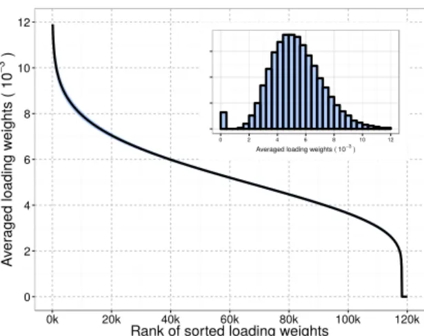
train and (right) test algorithms. . . 30 3.7 Loading weights distribution for a 120,059-dimensional feature vector (small

plot) and ranked in decreasing order (big plot). . . 32 3.8 (a) VIP measure and (b) Regression coefficient distribution for a 120,

059-dimensional feature vector (small plot) and ranked in decreasing order (big plot). . . 34

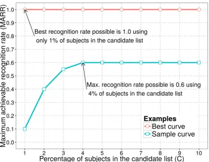
4.1 An example of the plots regarding the MARR evaluation metric for two sample curves. . . 37 4.2 Number of dimensions in PLS hash models and time spent to train 150 hash

models. . . 38 4.3 (a) Single features when 1% of the candidate list is provided for

4.4 Number of hash models as a function of the MARR for different percentages of subjects in the candidate list. . . 44 4.5 Contrast between binary counting sequence and random partition used in

the PLSH bit assignment. . . 45 4.6 Evaluation of the parameterp used for partitioning subjects in the gallery.

The theoretical optimal value forp is 0.5. . . 46 4.7 Evaluation of the partition number. . . 47 4.8 Comparison between score combination using product and sum. . . 48 4.9 Comparison of vote values in (a) projection based on the standard

multi-variate normal distribution (N(0, I)) and (b) PLSH. N(0, I) is employed in LSH methods to approximatel2 distances. . . 49 4.10 Average MARR and standard deviation for 10 PLSH runs considering 1%

of subjects in the candidate list. . . 50 4.11 Average MARR and standard deviation for 10 ePLSH runs considering 1%

of subjects in the candidate list. . . 51 4.12 Evaluation of loading weights, variable importance on projection (VIP) and

regression coefficients for feature selection. . . 52 4.13 MARR with different numbers of hash models and the feature selected in

ePLSH. . . 53 4.14 Number of hash models necessary to provide at least 0.95 MARR with

different gallery sizes and 1% of subjects in the candidate list. . . 54 4.15 Results on the FERET dataset. (a) PLSH MARR curves, (b) PLSH rank-1

recognition rate, (c) ePLSH MARR curves and (d) ePLSH rank-1 recogni-tion rate. . . 55

A.1 PLS sample code in R language used to discriminate Virginica from others flowers in the IRIS dataset. This code was used to generate Figure 3.2. . . 72

List of Tables

List of Algorithms

1 NIPALS(Xn×d, Yn, p) . . . 22

2 FaceIDlearn(Xn×d, In) . . . 25

3 FaceIDtest(x1×d) . . . 25

4 PLSHlearn(Xn,d, In, H) . . . 26

5 PLSHtest(x1×d) . . . 26

6 ePLSHlearn(Xn×d, In, H, k) . . . 30

List of Acronyms

CCA canonical correlation analysis

BRIEF binary robust independent elementary features

BRISK binary robust invariant scalable keypoints

CLBP circular local binary patterns

ePLSH extended PLS for face hashing

FAST features from accelerated segment test

FERET facial recognition technology

FREAK fast retina keypoint

FRGC face recognition grand challenge

HOG histogram of oriented gradients

ITQ iterative quantization

LBP local binary patterns

LDA linear discriminant analysis

LDE linear discriminant embedding

LFW labeled faces in the wild

LLE locally linear embedding

LSH locality sensitive hashing

MARR maximum achievable recognition rate

NN nearest neighbors

ORB oriented FAST and rotated BRIEF

PCA principal component analysis

PLEB point location in equal balls

PLS partial least squares

PLSH PLS for face hashing

POEM patterns of oriented edge magnitudes

PQ product quantization

SIFT scale invariant feature transform

SRC sparse representation-based classification

SSH similarity sensitive hashing

SURF speeded-up robust features

SVM support vector machine

VIP variable importance on projection

VLAD vector of locally aggregated descriptors

Contents

Acknowledgments xi

Resumo xv

Abstract xvii

List of Figures xix

List of Tables xxi

List of algorithms xxiii

List of Acronyms xxv

1 Introduction 1

2 Literature Review 7

2.1 Face Identification . . . 7 2.1.1 Fast Face Identification . . . 9 2.2 Large-Scale Image Retrieval . . . 10 2.2.1 Tree-Based Approaches . . . 11 2.2.2 Locality-Sensitive Hashing . . . 13 2.2.3 Hamming-based Approaches . . . 15

3 Methodology 21

3.3.3 Computational Requirements . . . 28 3.3.4 Alternative Implementations . . . 29 3.4 Feature Selection for Face Hashing (ePLSH) . . . 29 3.4.1 Loading Weights . . . 32 3.4.2 Variable Importance on Projection . . . 33 3.4.3 Regression Coefficients . . . 33 3.5 Early-Stop Search Heuristic . . . 34

4 Experimental Results 35

4.1 Experimental Setup . . . 35 4.1.1 FERET Dataset . . . 36 4.1.2 FRGC Dataset . . . 36 4.1.3 Evaluation Metric (MARR) . . . 36 4.1.4 Number of Dimensions in the PLS models . . . 37 4.1.5 Feature Descriptors . . . 38 4.2 PLSH Parameter Validation . . . 42 4.2.1 Combination of Different Feature Descriptors . . . 42 4.2.2 Number of Hash Models . . . 43 4.2.3 Balanced Partitions and Code Distribution . . . 44 4.2.4 Number of Random Partitions . . . 46 4.2.5 Voting Scheme . . . 47 4.2.6 Characterization of the Vote-List . . . 48 4.2.7 Stability of the Results . . . 49 4.3 ePLSH Parameter Validation . . . 50 4.3.1 Stability of the Results . . . 50 4.3.2 Feature Selection . . . 51 4.3.3 Number of Hash Models and Selected Features . . . 51 4.3.4 Number of Hash Models and Gallery Size . . . 53 4.4 Results on the FERET Dataset . . . 55 4.5 Results on the FRGC Dataset . . . 56

5 Conclusions and Future Works 59

Bibliography 61

A Partial Least Squares Example in R 71

Chapter 1

Introduction

According to Chellappa et al. [2010], there are three tasks in face recognition depending on which scenario it will be applied: verification, identification and watch-list. In the verification task (1 : 1 matching problem), two face images are provided and the goal is to determine whether these images belong to the same subject. In the identification task (1 : N matching problem), the goal is to determine the identity of a face image considering identities of subjects enrolled in a face gallery. The watch-list task (1 : N matching problem), which may also be considered as an open-set recognition task [Wechsler, 2009], consists in determining the identity of a face image, similar to the identification task, but the subject may not be enrolled in the face gallery. In this case, the face recognition method may return an identity in the face gallery or a not-enrolled response for any given test sample.

In this dissertation, we focus on the face identification task. Specifically, the main goal is to provide a face identification approach scalable to galleries consisting of numerous subjects and on which common face identification approaches would probably fail on responding in low computational time. There are several applications for a scalable face identification method:

• In a surveillance scenario consisting of numerous cameras spread throughout a large area and with hundreds of people passing every minute, such as in a large city, airport or sport events, the face identification should be able to return iden-tities from a potential large number of suspects fast enough such that authorities have a chance to respond in an emergency case.

2 Chapter 1. Introduction

Generic Face Identification

Face Representation

is not subject A/ is subject A

is not subject B/ is subject B

is not subject C/ is subject C Feature vector Face description Classification Subject A model Subject B model Subject C model Proposed Approach Face Representation

is not subject A/ is subject A

is not subject B/ is subject B

is not subject C/ is subject C Feature vector Face description Classification Subject A model Subject B model Subject C model Filtering Filtering Approach Subject is A or B

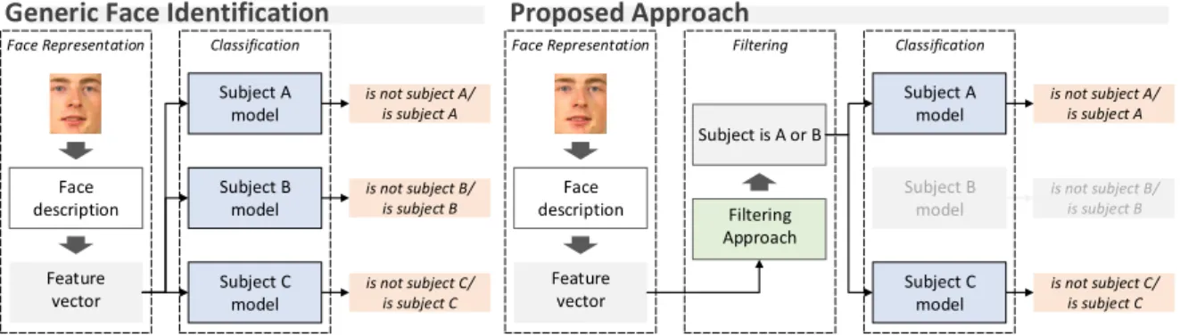
Figure 1.1: Common face identification pipeline and the proposed pipeline with the filtering approach which is used to reduce the number of evaluations in the classification step with low computational cost. The filtering approach is the main contribution in this work and it is tailored considering recent advances in large-scale image retrieval and face identification based on PLS.

could be used in an online system to store profiles and preferences for world-wide users and for fast identifying them and loading their data anyplace in the world.

• In social media, such as tagging people faces automatically in images, the face identification must be able to respond fast since slow websites tend to reduce the number of visitors [Brutlag, 2009].

The few aforementioned applications show the importance of performing face identification fastly and, in fact, several works in the literature have been developed in the past years motivated by these same types of applications (surveillance, forensics, human-computer interaction, and social media). However, most of the works focus on developing fast methods to evaluate one test face and a single subject enrolled in the gallery. These methods usually develop low computational cost feature descriptors for face images that are discriminative and with low memory footprint enough to process several images per second. Note that these methods still depend on evaluating all subjects in the face gallery. Therefore, if the number of subjects in the gallery increases significantly, these methods will not be able to respond fastly and new methods shall be developed to scale the face identification to this larger gallery.

3 Q Q Q Q Q Q Q Q A A A A A A A A B B B B B B B B C C C C C C C C D D D D D D D D E E E E E E E E F F F F F F F

F GGGGGGGG α α α α α α α α β β β β β β β β -1.0 -0.5 0.0 0.5 1.0

-1.0 -0.5 0.0 0.5 1.0

(a) Q Q Q Q Q Q Q Q A A A A A A A A B B B B B B B B C C C C C C C C D D D D D D D D E E E E E E E E F F F F F F F F G G G G G G G G -1 0 1

-1.0 -0.5 0.0 0.5 1.0

α

β

(b)

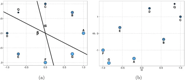
Figure 1.2: LSH idea illustration. (a) Random directionsα and β in the original space (b) and the projected samples. The goal is to find the enrolled samples D andC from the query sample Q, which can be accomplished considering the projections α and β.

identification by eliminating identities that are somewhat clearly not the identity in the test sample. Figure 1.2a illustrates the common face identification pipeline employed in practice and the main component tackled in this dissertation.

There is an extensive literature of works regarding large-scale image retrieval that could be employed in face identification. However, most of these works focus on re-turning a list containing images from the dataset that are similar to the test image. Although reasonable to recover images in large datasets, such approaches are not suit-able to apply directly to the face identification task. The models from subjects in the face gallery should optimally be described regarding the discriminative features related to each subject identity, which might consume less memory, specially if several sam-ples per subject are available, and less computational time, since only discriminative features are evaluated to determine the face identity.

Note that we do not claim to solve all of the aforementioned problems, but we hope to provide in this work some details for the future development of scalable face identification and a practical -but not optimal- alternative for the methods presented in the literature. The proposed approach is inspired by the family of methods regarded as

4 Chapter 1. Introduction

The main goal in LSH is to approximate the representation of samples in the high dimensional space using a small binary representation where the search can be implemented efficiently, employing a hash structure to approximate near-identical bi-nary representations. The idea in LSH is to generate random hash functions to map the feature descriptor in the high dimensional representation to bits in the binary representation.

As an example of LSH, suppose that we have a two dimensional query sample Q

and samplesAtoGenrolled in the gallery (see illustration in Figure 1.2a). The goal is to find the closest samples toQusing thel2 distance metric (Euclidian distance), which are C and D. In LSH, the search for the nearest neighbors considering the l2 distance metric is approximated by generating random projection vectors in which each element is drawn from a standard normal distribution. The idea is that, if two samples are close in the high dimensional space (similar vectors), they will almost surely be projected to similar values using the random projection vector. For instance, in Figure 1.2a, we select the orientation of a projection line α from a standard normal distribution and present the projected samples in the horizontal axis of Figure 1.2b. However, this is not always the case as some distant samples will also be projected to the same value as close samples. The random projection αin Figure 1.2 does not separate the sample B

fromQ, which are far apart in the original space. In this case, it is necessary a second projectionβ along withα to separateB fromQ.

In the PLSH approach, the random projection in the aforementioned example is replaced by PLS regression, which provides discriminability among subjects in the face gallery and allow us to employ a combination of different feature descriptors to generate a robust description of the face image. PLSH is able to provide significant improvement over the brute-force approach (evaluating all subjects in the gallery) and compared to other approaches in the literature. Furthermore, since the evaluation of hash functions in PLSH requires a dot product between the feature and regression vectors, additional speedup can be achieved by employing feature selection methods, resulting on the extended version of PLSH (ePLSH). The following contributions are presented in this work.

• A fast approach for face identification that support a combination of several feature descriptors and high dimensional feature vectors.

5

• Extensive discussion and experimentation regarding alternative implementations that may guide future development in scalable face identification methods.

• The proposed approach is easy to implement and to deploy in practice since only two trade-off parameters need to be estimated.

Chapter 2

Literature Review

This chapter reviews works related to face identification (Section 2.1) and large-scale image retrieval (Section 2.2). The goal of this chapter is to provide a background necessary to understand the development of the proposed approach and not a com-prehensive literature review of face identification and large-scale image retrieval. The reader may find more information regarding face identification in the book titled Hand-book of face recognition [Li and Jain, 2011]. For large-scale image retrieval, we re-fer the reader to the work [Wang et al., 2014a], regarding locality-sensitive hashing, and [Muja and Lowe, 2014], about search trees.

2.1

Face Identification

Face identification methods consist generally of two components: classifier and face representation. The classifier is responsible for receiving the face representation and returning an identity in the gallery, more specifically, it evaluates whether a face rep-resentation from a test image refers to a subject in the face gallery.

8 Chapter 2. Literature Review

Early works on face identification focused on subspace representation to tackle issues related to high dimensionality, correlation among pixels and noise [Sirovich and Kirby, 1987; Belhumeur et al., 1997]. In this case, the subspace is calculated considering compact description of samples for the same subject using principal component analysis (PCA) and maximum distance between samples from different subjects using linear discriminant analysis (LDA). Basri and Jacobs [2004] showed that lightning conditions in face images can be represented in less than 10 dimensions in a PCA-like subspace of gray-scale images. However, the aforementioned linear transformations to subspaces are not enough to capture all possible variations of faces. For this reason, image feature descriptors are considered in face identification.

Feature descriptors provide a robust manner to represent face images invariant to misalignment, illumination and pose of the face. Regard-ing feature descriptors considered in face identification, the most commons are local binary patterns (LBP) [Xie et al., 2012; Klare and Jain, 2013], Gabor filters [Gu et al., 2012; Oh et al., 2013] and descriptors based on gradient im-ages [Vu et al., 2012; Liao et al., 2013]. These feature descriptors capture mainly texture and shape of the face image, which are relevant for face identifica-tion [Schwartz et al., 2012]. There are two manners to represent the face im-age [K¨am¨ar¨ainen et al., 2011]: appearance-based (holistic), where the whole face image is represented in a feature descriptor vector; and feature-based (local), where fiducial points of the face image, such as nose tip or corners, eyes and mouth, are represented instead of the whole image.

The advantage of the holistic representation is the rich and easy encoding of the overall appearance of the face image. Since every pixel value contributes somehow to the final feature descriptor, more information is available to distinguish between samples from different subjects. However, preprocessing is usually necessary to cor-rect misalignment, illumination and pose. Feature descriptors commonly employed in holistic methods are the local binary patterns (LBP) [Xie et al., 2012], Gabor fil-ters [Gu et al., 2012], combination of both [Salah et al., 2013], and large feature sets coupled with dimension reduction techniques [Schwartz et al., 2012].

2.1. Face Identification 9

Fiducial points can be detected considering salient regions in the face image, which include corners and textured regions in the face. These salient regions, opposed to homogeneous regions such as cheek and forehead, tend to be stable among face images in different poses and lightning conditions. However, a method to match the detected salient regions among face images is necessary to compare feature descriptors. Liao et al. [2013] employ the popular SIFT [Lowe, 2004] to detect and match salient regions among face images. Another option is to learn common detectors for fiducial points (eye corner, nose tip, among others) such that the match of fiducial points among face images is no longer necessary since feature descriptors from a common type of fiducial point can be directly compared [Valstar and Pantic, 2012].

In the past few years, a different approach based on sparse representation-based classification (SRC) has been providing high accuracy in face identification datasets [Wright et al., 2009]. SRC consists in representing a test face image as a linear combination of a dictionary of images, which is learned using samples in the face gallery. Although the original proposal of SRC requires a fair number of controlled samples per subject for training, Deng et al. [2013] extended SRC to cope with few uncontrolled samples in the face gallery.

2.1.1

Fast Face Identification

Fast face identification is not a largely explored research topic and there are few works in the literature about it [Barkan et al., 2013; Deng et al., 2012; He et al., 2014; Yuan et al., 2005; Schwartz et al., 2012]. In [Barkan et al., 2013], compact descriptors based on local binary patterns are used to compare fastly the candidates in the face gallery. In [Deng et al., 2012] and [He et al., 2014], a fast optimization algorithm is considered for SRC to reduce the computational cost when calculating the linear combination be-tween the test and the samples in the dictionary. Although the aforementioned methods provide significant improvement on the test-subject comparison, poor performance is observed when there are numerous subjects in the face gallery since these approaches still present linear asymptotic complexity with the gallery size.

10 Chapter 2. Literature Review

The approach proposed in this dissertation is an extension of the work [Schwartz et al., 2012] and the main difference is the employment of hashing instead of search trees. PLS is also considered with a combination of feature descriptors as in Schwartz et al. [2012], which improves the face identification recognition rate com-pared to single feature descriptors. In this case, the contribution of the proposed approach lies in the distinct manner in which PLS is employed for hashing and the considerable improvement in speedup compared to the aforementioned scalable face identification approaches.

2.2

Large-Scale Image Retrieval

The goal in the image retrieval task is to return a sorted list of “relevant” images enrolled in the gallery considering their similarity to a test sample. The common as-sociated task, referred to as k-NN, consists in calculating distances between test and gallery samples and returning the first k closest samples. The brute-force k-NN ap-proach consists in calculating all the distances between the test and gallery samples and sorting them, which is unfeasible for large galleries. In this case, efficient sub-linear al-gorithms to solve thek-NN task are employed. An example iskd-tree [Gan et al., 2007], which consists in splitting recursively the space in subregions and organizing them in a hierarchical structure that provides averaged asymptotic complexity O(log(n)) for a given gallery size n. Although kd-tree considers only the l2 distance metric, it is possible to extend the idea to other distance metrics [Uhlmann, 1991].

The main reason of the poor performance related to distance-based approaches in high dimensional data is the small difference among distance values, which hampers the analyses of which samples are similar or dissimilar (both will present almost the same values). Furthermore, axis-oriented splits employed inkd-trees are not sufficient to ap-proximate nearest neighbor search in the high dimensional space [Ch´avez et al., 2001]. In this case, the solution is embedding feature descriptors in a low dimensional space where conventional distance metrics return relevant values.

2.2. Large-Scale Image Retrieval 11

There exists a decision problem related tok-NN, regarded asr-nearest neighbors (r-NN), which is more tractable and efficiently approached thank-NN. Ther-NN task can be reduced to k-NN using a binary-search approach [Har-Peled, 2001] and consists in returning all samples in the gallery that are within a fixed radius distance r from the test sample. The approximated version of r-NN, regarded as (r, c)-NN, consists in returning all samples within a distance at most rc from the test sample. In this case, the parameter cis important to delimiter regions in the feature space where it is possible to determine the worst case scenario for retrieving samples within r.

There are several approaches for large-scale image retrieval in the literature. How-ever, a complete review and description of all types of approaches is out-of-scope in this work. Instead, we focus on past works that have been successfully applied to face identification. In this context, tree-based approaches are described in Section 2.2.1, locality-sensitive hashing in Section 2.2.2, and Hamming embedding-based approaches in Section 2.2.3.

2.2.1

Tree-Based Approaches

Large-scale image retrieval based on search trees consists in partitioning recursively the samples and organizing them in the partitions using a tree structure. In this way, the organization of samples is hierarchical, with the higher level (root node of the tree) representing the full sample set and lower levels (leafs) representing subsets of samples. The number of levels in the tree (l) depends on the number of samples (n), the number of partitions in each level (p), and whether the number of samples in each partition is the same (balanced partitions), in which case l = ⌈logp(n)⌉. Unbalanced partitions

lead to l = n, in the worst case. Controlling l is important since the computational cost to traverse the tree from the root node to a leaf has asymptotic complexity O(l).

Partitioning is the main component of the search tree and it determines the effectiveness of the tree approach to balance partitions (reduce l) and to guide the search towards most likely nearest neighbors (reduce traversals). However, it is rarely possible to split real data in balanced partitions based on common features among samples within each partition. For instance, gender, ethnicity and age are hardly balanced among subjects in a specific group (engineer students, politicians, travelers, among others). Nevertheless, balanced partitions can be forced using random split of samples at the cost of traversing the tree a few times to find the nearest neigh-bors [Schwartz et al., 2012].

12 Chapter 2. Literature Review

each partitioning to reduce, or eliminate, the influence of redundant, irrelevant and noisy features. Another option is to employ partitioning approaches based on robust classifiers, such as SVM [Pang et al., 2005] and PLS [Schwartz et al., 2012], which pro-vide good performance even with noisy and redundant features. The disadvantage of these approaches is the higher computational cost to traverse each node in the tree (O(d), where d is the dimensionality of the data) compared to axis oriented partition-ing (O(1)) [Wang et al., 2014b].

The following approaches employ partitioning considering maximum vari-ance directions in the feature space based on the work of Sproull [1991]. Silpa-Anan and Hartley [2008] employ a similar approach, but considering multiplekd -trees and a shared priority queue, which determines the order to evaluate samples for nearest neighbors candidates. An improvement of computational cost is achieved con-sidering a feature subset, since akd-tree usually considers few features to split samples and the exact samekd-tree is obtained using only these features. Wang et al. [2014b] employ hyperplanes considering elements with values 1, 0 and−1 to reduce the com-putational cost to evaluate nodes in the tree presenting asymptotic complexity O(d) for hyperplanes inRd_{. The approach also employs numerous trees, learned considering}

a subset of features selected randomly with probability proportional to its variance in the training samples.

Random projections are an alternative approach compared to maximum vari-ance directions and usually provide competitive results as demonstrated in the fol-lowing approaches. Dasgupta and Freund [2008] employ the median value of the sam-ples projected in the random direction as threshold, which generates a balanced tree. Liu et al. [2004] employ the mean value of the most distant values projected in the random subspace as threshold and allow samples to be shared among node children, which increase the number of levels in the tree but reduce the number of traversals in general. In this case, the speedup is obtained since less node evaluations are necessary, which has the same computational cost of evaluating one sample for nearest neighbor (asymptotic complexityO(d)).

2.2. Large-Scale Image Retrieval 13

2.2.2

Locality-Sensitive Hashing

Locality-sensitive hashing (LSH) refers to a family of embedding approaches (see Sec-tion 2.2.3 for a brief descripSec-tion of embedding) that aims at mapping similar feature descriptors to the same hash table bucket with high probability while keeping dissim-ilar features in different buckets. LSH approaches provide logarithm asymptotic com-plexity in time and linear comcom-plexity in space. Indyk and Motwani [1998] were the first to introduce the term locality-sensitive hashing in 1998. However, Broder [1997] was the first to describe a LSH approach (min-hash) in 1997 to cluster and to detect near-duplicated web pages. Since then, several approaches has been proposed in the literature to include different domains in the LSH framework. A summary of numerous LSH approaches can be found in [Wang et al., 2014a].

An approach is regarded as being LSH, with arguments r, c, p1, p2 (p1 > p2), if the hash function h(x) employed belongs to a family of hash functions H, which approximates the distance metric d(p, q) of the feature descriptors p and q in the following manner:

if d(p, q)≤r then P r h(p) = h(q) ≥p1, if d(p, q)≥cr then P r h(p) = h(q)

≤p2,

where P r denotes probability and r denotes the maximum distance d(p, q) that maps

p and q to the same bucket with minimum probability p1. The second case ensures that distant feature descriptors (d(p, q) ≥ cr) has low probability (p2) to be mapped into the same bucket for a constant c > 1. The LSH considers the (r, c)-NN task and, in practice, it can be employed directly instead of k-NN by setting r according to the desired precision and recall of the samples retrieved and maximum approximation error equal to ǫ, where c= (1 +ǫ).

LSH employsK hash functions{h1, ..., hK}selected independently and uniformly

from H. Raising K provides higher precision in practice, but increases the size of the hash table and reduces recall. For this reason, hash functions are usually grouped in

L groups {g1, ..., gL} of K hash functions (gi = {hi,1, ..., hi,K}), resulting in L hash

tables and LK hash functions in total. Raising L is known to improve recall, but the values of L and K are bounded by the computational cost of hashing features in practice. IfK is set tolog1/p2(n) andLis set ton

ρ_{, whereρ=log(1/p1)/log(1/p2),the}

LSH framework generates algorithms with asymptotic space complexity O(dn+n1+ρ_),

n and d denote number and dimensionality of the samples, respectively, and time complexity bounded byO(nρ_{) similarity calculations andO(n}ρ_log

1/p2(n)) hash function

14 Chapter 2. Literature Review

In practice, given r, c → 1 is desirable, although c too small reduces preci-sion (p2 increase), which is compensated by generating more hash functions (given by log1/p2(n)). For example, Datar et al. [2004] calculate ρ = 1/c considering hash

functions sampled from a p-stable distribution to approximate the l1 or l2 distance metrics, which is close to the lower theoretical limit ρ → 1/2c [Motwani et al., 2007]. The approximation factor can also be calculated using Monte Carlo for complex hash functions [Terasawa and Tanaka, 2007].

There are two types of hash functions in LSH [Wang et al., 2014a]: data inde-pendent, where hash functions are defined regardless of the data; and data dependent, where the parameters of the hash functions are selected according to the training data. These two types are different from supervised and unsupervised learning of hash func-tions, in which the difference lies on whether data label is considered. For instance, data dependent hash functions may not consider the label of the data when learning hash functions. However, all supervised hash functions are intrinsically data dependent, since the family of hash functionsH will be selected to discriminate labels.

Data independent hash functions are employed in the works of Datar et al. [2004], based on p-stable distributions; Chum et al. [2008], based on min-hash; Joly et al. [2004] and Poullot et al. [2007], both works based on space filling curves. Data independent hash functions are usually employed in heterogeneous data like in the object recognition task. In this case, the overall distribution of the data is not modeled easily using data dependent hash functions. For instance, the distribution of a common object (more samples) may outweigh uncommon objects (few samples). In this case, unsupervised data dependent functions will be biased toward representing the sample distribution of the common object. Other advantages of the data independent hash functions are the fast learning process, which is independent from the gallery size, and the enrollment of new samples, which does not require retraining hash functions.

2.2. Large-Scale Image Retrieval 15

There are numerous LSH approaches for different metric spaces. The most common applications include LSH approaches for lp metric space [Datar et al., 2004]

based on p-stable distributions; random projections [Andoni and Indyk, 2006], which approximate cosine distances; Jaccard coefficient [Broder, 1997]; and Hamming dis-tances [Indyk and Motwani, 1998], where the goal is to provide approximated nearest neighbors as opposed to exact nearest neighbors as presented in Section 2.2.3.

It is important to emphasize that the proposed approach is not included in the LSH family. We do employ hash functions generated independently from each other and the proposed approach considers data labels, but there is no associated distance metric and, therefore, no approximated k-NN solution. We focus on returning correct identities in a shortlist of candidates rather than approximating nearest neighbors in a given metric space. The proposed approach also behaves similarly to LSH methods, where the increase in the number of hash functions provides improved results, but we cannot prove the approximation limits of the proposed approach in the same way as in LSH. In our experiments, we notice that the results never exceed the recognition rate of the brute-force based on PLS, which might indicate that the proposed method approximates the results from PLS-based approaches.

2.2.3

Hamming-based Approaches

The most common approach in large-scale image retrieval consists in embedding feature descriptors in a low dimensional space where locality is preserved (simi-lar feature descriptors have simi(simi-lar representation in the low dimensional space) and where nearest neighbor search can be implemented efficiently. This section fo-cuses on embedding feature descriptors in the Hamming space, which is widely used in the literature and consists in the space spanned by a set of 2S _{binary strings}

with length S. Other options for embedding include linear discriminant embedding (LDE) [Chen et al., 2005], LDE variation [Hua et al., 2007], or embedding in Huff-man trees [Chandrasekhar et al., 2009, 2012]. The difference between tree-based search (Section 2.2.1) and embedding feature descriptors in Huffman trees is the hierarchical organization of samples in the former compared to sample encoding in the latter.

16 Chapter 2. Literature Review

The main advantages of Hamming space embedding are the low memory require-ment (one binary string for each sample) and the efficient implerequire-mentation of Hamming distance using bitwise operations (xor operation between two strings followed by a small code to count number of bits equal to one). Given the importance of operations in the Hamming space, specially in cryptography and error detection, CPU manufac-tures included an instruction to compute efficiently the number of bits equal to one in the instruction set (POPCNTSSE4.2). For the purpose of completeness and clear understanding of this work, the same notation of the Hamming distance employed by Bronstein et al. [2011] is considered. In this case, Hamming distance is defined as

d(X, Y)H =

S

2 − 1 2

S X

i=1

sgn(xiyi),

in the spaceHS _={−1,+1}S_{, which is equivalent to the number of different elements}

in the strings X ={x1, ..., xS} and Y = {y1, ..., yS}. The function sgn(a) returns +1

if a is positive and−1, otherwise.

There are two tasks to retrieve nearest neighbors in the Hamming space [Norouzi et al., 2012]. One task, referred to as k-nearest neighbors (k-NN), con-sists in retrieving a fixed number of samplesk with minimum distance to the test sam-ple. The other task, referred to as approximate query or point location in equal balls

(PLEB) [Indyk and Motwani, 1998], consists in retrieving all samples within a fixed maximum distance r to the test sample. There is no better way to retrieve samples in the k-NN task than evaluating all distances between the test and gallery samples and, although k-NN is unfeasible in practice, it is useful to access the recall among Hamming embedding methods [He et al., 2013; Gong et al., 2013; Wang et al., 2012].

The approximate query approach may be implemented using hash table where samples are indexed in multiple positions according to r. In this case, the limitations are the memory necessary to allocate the hash table (viable only for smallS) and the large number of samples retrieved and indexed multiple times, which is proportional exponentially tor. The number of hash table positions visited is given by

v(r, S) =

r X

i=0

S i

1_.

Even a reasonable value for r and S may represent a search for hash table positions higher than the gallery size. For instance,r = 4 andS = 128 result inv = 11,017,633. Furthermore, the memory necessary to allocate the hash table with 128 bits would be

1

2.2. Large-Scale Image Retrieval 17

at the order of undecillions. In this case, Norouzi et al. [2012] proposed an approach that approximates the query task by employing indexing of non-overlapping substrings in multiple hash tables to avoid the aforementioned issues.

Numerous approaches have been proposed in the literature to map feature de-scriptors in the Hamming space. Most of them are based on optimization such as minimizing the quantization error. The supervised optimization version consists in minimizing the distance of same-class feature vectors in the Hamming space while maximizing the distance of feature descriptors from different classes. In this case, elements in the Hamming string present different discriminative performances and a weighted distance version, such as

dw(X, Y)H =

S

2 − 1 2

S X

i=1

αisgn(xiyi), (2.1)

provide better results. The weights αi can be learned using an adaptive learning

algorithm, as depicted in [Shakhnarovich, 2005].

Regarding unsupervised approaches, J´egou et al. [2012] employ quantization of feature descriptors considering a random rotation of the PCA transformation to ensure equal variance among projected features. In the unsupervised version, Gong et al. [2013] employ a similar approach but considering the minimal quantiza-tion error of zero-mean samples in a zero-centered binary hypercube. In this case, an efficient optimization algorithm can be formulated, referred to as iterative quan-tization (ITQ), which provides better results than the random rotation employed in [J´egou et al., 2012]. He et al. [2013] show that competitive results can be ob-tained by employing the minimization of the error in the Hamming embedding in-stead of squared error in thek-means algorithm used in theproduct quantization (PQ) method [J´egou et al., 2012]. Norouzi and Blei [2011] employ maximum-margin opti-mization between dissimilar quantized feature descriptors, which is carried following an neural network optimization algorithm according to an upper-bound function.

Regarding supervised or semi-supervised Hamming embedding, approaches based on metric learning have been the most common in the literature. Most of them can be formulated following the similarity sensitive hashing (SSH), described in [Shakhnarovich, 2005] and defined as xi = sgn(wif +bi), where each bit xi in the

Hamming space depends on f, which is ad-dimensional feature descriptor, wi denotes

d-dimensional metric parameters and bi is bias (zero for mean centered data).

18 Chapter 2. Literature Review

(CCA) rather than PCA in the ITQ method. Wang et al. [2012] propose to learn the quantization separately for each bit and incorporate correction of weak quantized bits when learning new ones. Jain et al. [2008] employ random directions weighted by Mahalanobis distance. Strecha et al. [2012] employ LDA, which maximizes the inter-class distance and minimize the intra-inter-class variance. Bronstein et al. [2011] employ an optimization similar to LDA, but considering an exponential loss function appropriated to the bag-of-words model. We refer the reader to the work of Wang et al. [2012] for a summary table of SSH-based approaches.

Approaches other than SSH-based include the work of Liu et al. [2012], which employs kernel function optimized to consider minimum same and maximum not-same Hamming distances between classes. Another option is to employ deep learning algo-rithms, which have been an active research topic in recent years. In this case, the same principles adopted in Hamming embedding methods are employed in the neural net-work. For instance, the goal in deep learning based methods is to represent the whole image in a compact binary string. One of the challenges in considering deep learning approaches is the high computational cost induced by convolutional layers, which can be significantly reduced when related regions not related to the object in the image are discarded (background and homogeneous regions) [Mopuri and Babu, 2015]. Al-though simple, this approach provide better results than well-known methods such as the vector of locally aggregated descriptors (VLAD) [J´egou et al., 2012].

The optimization step in the neural network can also be tailored to min-imize reconstruction loss from the binary string, distribute uniformly the binary string and provide strings with maximum independence among bits (reduce redun-dancy) [Erin Liong et al., 2015]. The method can be further extended to consider labels, in which the probability of samples with different labels receiving the same binary code is minimized while samples with same labels receiving the same bi-nary code is maximized Lin et al. [2015]. Similar to the aforementioned works, Torralba et al. [2008] employ deep learning (four or five layers in the neural network hidden algorithm depending on the string length) to map same label samples in the same string.

2.2. Large-Scale Image Retrieval 19

The best Hamming-embedding methods, in general, consider four optimization strategies. First, a balanced set of bits, which tends to distribute Hamming strings (hash codes) uniformly among samples in the dataset. Second, independency among bits, which provide shorter Hamming strings. Third, minimization of the quantization lost, which ensure that locality in the high dimensional representation of the image is preserved in the Hamming embedding space. Finally, since each bit in the Hamming string may contribute differently for the image retrieval accuracy, annotated data could be employed to weight bits according to their retrieval capability.

Chapter 3

Methodology

This chapter describes the methods employed in the proposed approach, namely PLS for regression (Section 3.1) and PLS for face identification (Section 3.2). The proposed PLSH is described in Section 3.3 and in Section 3.4, we describe a PLSH extension (ePLSH), which consists in employing PLS-based feature selection to improve the per-formance of PLSH.

3.1

Partial Least Squares Regression

PLS is a regression method that combines ordinary least squares applied to a latent subspace of the feature vectors. Several works have employed PLS for face identi-fication [Schwartz et al., 2012], face veriidenti-fication [Guo et al., 2011], and open-set face recognition [Santos Jr and Schwartz, 2014]. These works consider PLS mainly due to the robustness to combine several feature descriptors, capability to deal with thousands of dimensions, and robustness to unbalanced classes. In this work, we consider PLS due to the high accuracy presented when used to retrieve candidates in PLSH and the low computational cost to test samples since only a single dot product between the regression coefficients and the feature vector is necessary to estimate the PLS response. PLS is calculated as follows. The p-dimensional latent subspace is estimated by decomposing the zero mean matrices Xn×d, with n feature vectors and d dimensions,

and Yn, with response values, in

Xn×d =Tn×pPdT×p+En×d,

Yn×1 =Un×pQp×1+Fn×1,

(3.1)

22 Chapter 3. Methodology

Algorithm 1: NIPALS(Xn×d, Yn, p)

1 fori←1 to p do

2 startu_i randomly or with some column ofX

3 repeat

4 w_i ←XTu_i/kXTu_ik;t_i←Xw_i

5 q_i ←YTt_i/kYTt_ik;u_i←Y q_i

6 untilconvergence;

7 b_i←u_it_i/kt_ik;p_i←XTt_i/kt_ik 8 X←X−t_ipT_i ;Y ←Y −b_i(t_ipT_i )

9 return T, P, U, Q, W, B

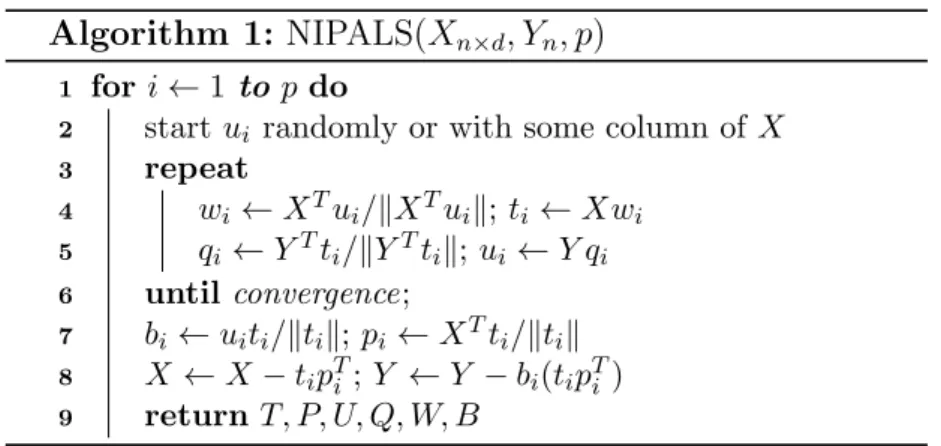
Figure 3.1: NIPALS algorithm. Xn×dand Yn denote feature vectors and target values,

respectively, withn samples and ddimensions. pdenotes number of dimensions in the PLS model.

respectively. The matrixPd×p and the vector Qp represent loadings and the matrixE

and the vectorF are residuals from the transformation. PLS algorithms computeP and

Qsuch that the covariance between U andT is maximum [Rosipal and Kramer, 2006]. We consider the nonlinear iterative PLS (NIPALS) algorithm [Wold, 1985] (presented in Figure 3.1) which calculates the maximum covariance between the latent variables

T ={t1, ..., tp} and U ={u1, ..., up} using the matrix Wd×p ={w1, ..., wp}, such that

arg max[cov(ti, ui)]2 = arg max |wi|=1

[cov(Xwi, Y)]2.

The regression vector β between T and U is calculated using matrix W according to

β =W(PT_W)−1_(TT_T)−1_TT_{Y. (3.2)}

The PLS regression response ˆy for a probe feature vector x1×d is calculated according

to ˆy = ¯y+βT(x−x¯), where ¯y and ¯x denote average values of Y and elements of X, respectively. The PLS model is defined as the variables necessary to estimate ˆy, which are β, ¯x and ¯y.

Efficient implementations of the NIPALS algorithm using graphical cards exist in the literature and they can provide speedup of up to 30 times compared to the CPU version [Srinivasan et al., 2010]. For prototyping, we recommend the PLS package in the R programming language [Mevik and Wehrens, 2007], which include different PLS versions and tools to analyze the model learned.

3.1. Partial Least Squares Regression 23

4

3 2 1 0 -1 -2 -3

3 2 1 0 -1-2 -2 -1 0 1 2 (a) -2 -1 0 1

-2 0 2 4

PLS first dimension

PLS second dimension

(b)

2 1 0 -1 -2 -3

3 2 1 0 -1 -2 -2 -1 0 1 2 (c) -1 0 1 2

-2 0 2 4

PCA first dimension

PC

A second dimension

(d)

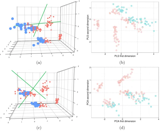
Figure 3.2: (a) PLS axis in 3-dimensional space and (b) features projected in the first two dimensions of PLS. (c) PCA axis in 3-dimensional space and (d) features projected in the first two dimensions of PCA. The goal is to separate Virginica flower samples (blue points) from other flower samples (red points). Note that, although PCA and PLS employ a similar transformation, the subspace generated by PLS discriminate better than PCA the two types of samples. Best visualized in color.

24 Chapter 3. Methodology

Filtering

Large-scale image retrieval

Candidates list

High probability Low probability

Subject C Subject D Subject B Subject A

[Feat1 ... Featf]

Feature extraction

Evaluate only high probability subjects in the face identification model

Face identification Subject C Subject D Subject B Subject A Test 3 1 2 5 4

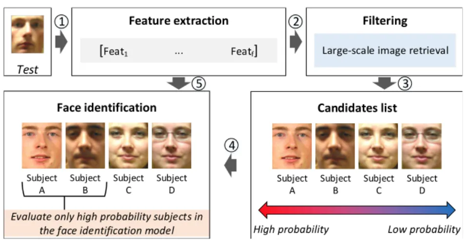
Figure 3.3: Overview of the filtering and the face identification pipeline. (1) Different feature descriptors are extracted from the test image and concatenated resulting in a large feature vector more robust to image effects than single feature descriptors. (2) The feature vector is presented to the filtering approach, which employs a large-scale image retrieval approach to (3) generate the candidate list sorted by the probability that the candidate is the subject in the test image. (4) A small percentage of the candidate list (high probability candidates) is presented to the face identification which will evaluate only the models relative to these candidates.

will be estimated. Note that if we use PCA (see Figures 3.2c and 3.2d), the subspace calculated will be different because PCA considers directions that explain most of the variance in the data. The script used to generate Figures 3.2a and 3.2b is available in Appendix A.

3.2

Face Identification Based on Partial Least Squares

3.2. Face Identification Based on Partial Least Squares 25

Algorithm 2:FaceIDlearn(Xn×d, In)

1 X←(X−µ)/σ 2 M ←∅

3 foreach unique id∈I do

4 Y ← {yi|yi =

(

+1, ifIi =id

−1, otherwise

5 W, P, T ←NIPALS(X, Y)

6 Calculateβ_idusing Eq. 3.2

7 M ∪ {(id, β_id)}

Algorithm 3: FaceIDtest(x1×d)

1 x←(x−µ)/σ

2 max← −∞

3 predict←“none”

4 for each(id, β_id)∈ Mdo

5 score←βT_idx

6 if score>maxthen

7 max←score

8 predict←id

9 return predict

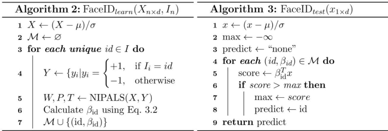
Figure 3.4: Original algorithm of the PLS face identification as described by Schwartz et al. [2012] with the (left) train and (right) test steps. Xn×d denotes

n feature vectors with ddimensions, In denotes labels for each feature vector and x1×d

denotes probe sample.

which evaluates subjects following the order in the candidate list until the face identifi-cation returns a subject in the face gallery. In this case, speedup is achieved because it is not necessary to evaluate the remaining subjects in the candidate list once a gallery match is found, reducing therefore, the computational cost compared to the brute-force approach. Note that we do not calculate the probability directly but we associate it with the estimated PLS regression values as will be presented.

There are two types of errors in the filtering and face identification pipeline. The first type of error is related to the filtering approach and occurs when the subject in the test sample is enrolled in the gallery, but is not in the candidate list, resulting in a miss for any face identification approach employed afterwards. The second type of error is related to the face identification approach and occurs whenever the test sample subject is within the candidate list but a wrong identity is assigned by the face identification approach.

To evaluate the filtering and face identification pipeline, we consider the face identification method described by Schwartz et al. [2012], which consists in employing a large feature set concatenated to generate a high dimensional feature descriptor. Then, a PLS model is learned for each subject in the gallery following aone-against-all

26 Chapter 3. Methodology

Repeat H Times

Gallery

Subject C Subject D Subject B Subject A

Random split

Positive set

|Sub. A|Sub. C|

Negative set

|Sub. B|Sub. D|

Subject indexes |Sub. A|Sub. C|

PLS Model

Vote-list

Repeat H Times

Subject indexes |Sub. A|Sub. C|

PLS Model R

Test S o rt a n d p re se n t a s ca n d id a te l is t Sub. A Sub. D Sub. C Sub. B T e s t L e a r n

Algorithm 4:PLSHlearn(Xn,d, In, H)

1 X←(X−µ)/σ 2 forh= 1 to H do

3 Y ←[−1, ...,−1]n;Ph←∅

4 foreach uniqueid∈I do

5 sampler from Bern. (p= 0.5)

6 if r=success then

7 Ph∪ {id}

8 Y ={yi|yi= 1, ifIi=id} 9 Calculateβh using Eq. 3.2

10 M ∪ {(Ph, βh)}

Algorithm 5: PLSHtest(x1×d) 1 x←(x−µ)/σ

2 V ← {(id1,0), ...,(idn,0)} 3 foreach(Ph, βh)∈ Mdo

4 score←βT_hX

5 V ← {(i, s)|s=s+ score, ifi∈ Ph}

6 V ← {(i, s)|s >0}

7 sort (i, s)∈V in decreasing order ofs

8 returnV

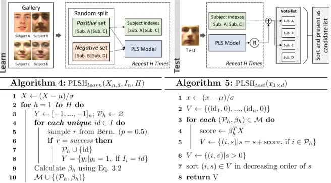
Figure 3.5: Overview of PLS for face hashing (PLSH) with (left) train and (right) test algorithms. Xn,d denotes samples, In are labels, H is number of hash models, x1×d

denotes probe sample andMdenotes hash model set (initially empty).

3.3

Partial Least Squares for Face Hashing (PLSH)

The PLSH method is based on two principles: (i) data dependent hash functions and (ii) hash functions generated independently among each other. Data dependent hash functions provide better performance in general (see discussion in Section 2.2.2). Hash functions generated independently are necessary to induce uniform distribution of binary codes among subjects in the gallery [Joly and Buisson, 2011]. A diagram and algorithm for PLSH is presented in Figure 3.5.

PLSH consists of two steps: train and test. In the train, we randomly split subjects in the gallery in two balanced subsets: positive and negative. The split is performed as follows. For each subject, we sample from a Bernoulli distribution with parameterp= 0.5 and associate the subject to the positive subset in case of “success”. PLS regression models are used to determine whether a test sample belongs to the positive or to the negative subset. In this case, the PLS regression model is learned considering feature descriptors extracted from samples in the positive set with target values equal to +1 against samples in the negative set with target values equal to−1. This process is repeated several times1_{.We define a PLSHhash model as a PLS model} and the subjects in the positive subset.

1

3.3. Partial Least Squares for Face Hashing (PLSH) 27

In the test, we extract the same feature descriptors employed on the train for the test sample (probe sample) and presented them to each PLSH hash model to obtain a regression value r. We define a vote-list of size equal to the number of subjects in the gallery initially with zeros, then, each position of the vote-list is increased by

r according to the indexes of subjects in the positive subset of the same PLSH hash model. Note that this scheme allows us to store half of the subject indexes to increment the vote-list since it will be equivalent to increment subjects in the negative set by |r|

when ris negative (the differences among pairs of votes will be the same). Finally, the list of subjects is sorted in decreasing order of values and presented as candidates for the face identification.

In practice, the majority of subjects with low values in the candidate list are discarded because they rarely corresponds to the test sample. The candidate list only serves to indicate the evaluation order for the face identification method. In this case, if an identity is assigned to the probe when evaluating the first candidates in the list, there is no need to evaluate the remaining candidates.

PLSH is similar to the work of Joly and Buisson [2011], in which SVM classifiers are employed to determine each bit in the Hamming embedding. The advantage of employing PLS in this case is the robustness to unbalanced classes and support for high dimensional feature descriptors [Santos Jr and Schwartz, 2014]. We do not provide approximation bounds to PLSH as LSH methods because PLSH is based on regression scores rather than distance metrics, which are not compatible with the LSH framework.

3.3.1

Consistency

The motivations for the steps presented in the PLSH algorithm are the following. In one hand, ifris approximately equal to +1 in the test, the probe sample is more similar to the subjects in the positive subset and the positions in the vote-list corresponding to the subjects in the positive subset will receive more votes. On the other hand, if

28 Chapter 3. Methodology

even if the correct subject is in the positive subset and the increase in the number of hash functions is limited only by the computational cost to evaluate them.

3.3.2

Hamming Embedding

We do not estimate the Hamming embedding directly since there is no binary string associated to any face sample. However, PLSH is equivalent to estimating the Hamming embedding for a test sample and comparing it with the binary strings generated for each subject in the gallery. In addition, each bit of the test binary string is weighted by the absolute value of the PLS regression response. To demonstrate the aforementioned claims, consider that PLS responses can be only +1 or −1, such that any test sample can be represented by the sequence X = {+1,−1}H_{, where H denotes the number of}

PLSH hash models. Consider also that each subjects in the face gallery is represented by the binary string Ys = {1,0}H, where yi ∈ Ys is set to 1 if the subject s was

associated to the positive subset of the i-th PLSH hash model in the train step, or 0, otherwise. In this context, the weightws given by PLSH to each subject in the gallery

is calculated as

ws = H X

i=1

xiyi.

Note that the maximum ws is equal to the sum of +1 elements in X, which occurs

when yi = 1, if xi = +1, and yi = 0, otherwise. Similarly, the minimum weight is

equal to the sum of −1 elements in X, which occurs when yi = 1, if xi = −1, and

yi = 0, otherwise. If we transform X onto a binary string ˆX such that ˆxi = 1, if the

correspondingxi is +1, and ˆxi = 0, otherwise; we can calculate the Hamming distance

between ˆX andYs. In fact, the exactly same Hamming distance can be calculate using

ws as

d(X, Y)H =w_max−w_s, (3.3)

where wmax denotes maximum possible ws. The same analogy can be applied to the

weighted Hamming distance (see Equation 2.1) if we consider xi assuming any real

number. In this case, the weight of each bit αi is the absolute value of r and the

weighted Hamming distance is equivalent to Equation 3.3.

3.3.3

Computational Requirements

3.4. Feature Selection for Face Hashing (ePLSH) 29

N. Each hash model holds a PLS regression vector in Rd _{and the indexes of subjects}

in the positive subset, given by N/2, therefore, H ×D real numbers and (H ×N)/2 integer indexes of space are necessary using H hash functions in the PLS algorithm. Note that it is not necessary to store the feature vectors used to train the PLS models in the test and they can be safely discarded since the PLS regression vector holds the necessary information to discriminate among the enrolled subjects.

3.3.4

Alternative Implementations

In principle, some aspects of the PLSH algorithm can be changed such that PLSH can provide potential performance improvement. For instance, the parameter p of the Bernoulli distribution used to determine the subsets of subjects may be changed given that PLS hardly finds common discriminative features among subjects in a large set Santos Jr and Schwartz [2014]. However, changingpfrom 0.5 to other value results in a nonuniform distribution of subjects among subsets (raise hash table collisions), therefore, reducing the accuracy. As will be demonstrated in the experiments, main-taining a balanced subset of subjects to learn each hash model (p= 0.5) provide the best results.

Another possible implementations of PLSH that does not modify much the results is the product of votes instead of the sum, which is akin to the intersection of subsets among all hash functions. It is also possible to employ multiple partitions instead of only two by using a categorical rather than Bernoulli distribution. However, multiple partitions provide no significant difference in the results and they require twice the space requirement since the indexes of subjects that were learned with +1 target re-sponse in the PLS model need to be stored to allow them to receive the votes in the test. At last but not least, the computational cost to evaluate the hash functions can be reduced when considering feature selection methods, which consists in calculating the PLS regression response using few dimensions in the feature vector corresponding to the most important to discriminate between the subject subsets. As will be presented, the feature selection include a new parameter in the PLSH algorithm, the number of features selected, which can be estimated jointly with the number of hash functions to provide much better results than in PLSH without feature selection.

3.4

Feature Selection for Face Hashing (ePLSH)

30 Chapter 3. Methodology

Repeat H Times Feature

selection

Gallery

Subject C Subject D Subject B Subject A

Random split

Positive set

|Sub. A|Sub. C|

Negative set

|Sub. B|Sub. D|

k top PLS features

Vote-list

Repeat H Times Subject indexes |Sub. A|Sub. C|

R Test S o rt a n d p re se n t a s ca n d id a te l is t Sub. A Sub. D Sub. C Sub. B T e s t L e a rn Subject indexes |Sub. A|Sub. C|

PLS Model

Selected features

PLS Model

Selected features

Algorithm 6:ePLSHlearn(Xn×d, In, H, k)

1 X←(X−µ)/σ 2 forh= 1 to H do

3 Y ←[−1, ...,−1]n;Ph←∅

4 foreach uniqueid∈I do

5 sampler from Bern. (p= 0.5)

6 if r=success then

7 Ph∪ {id}

8 Y ={yi|yi= 1, ifIi=id} 9 Fh←k discriminative features

10 select featuresFh from X

11 Calculateβh using Eq. 3.2 12 Me∪ {(Ph, βh, Fh)}

Algorithm 7: ePLSHtest(x1×d) 1 x←(x−µ)/σ

2 V ← {(id1,0), ...,(idn,0)} 3 foreach(P, βh, Fh)∈ Medo 4 select features Fh from x

5 score←βT_hx

6 V ← {(i, s)|s=s+ score, ifi∈ P} 7 V ← {(i, s)|s >0}

8 sort (i, s)∈V in decreasing order ofs

9 returnV

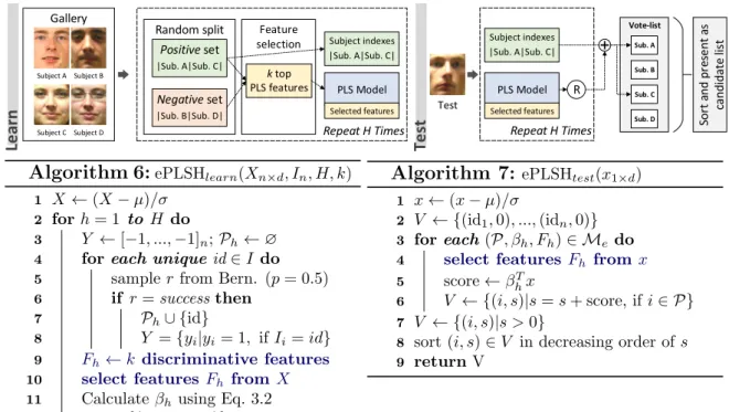
Figure 3.6: Overview of PLS for face hashing and feature selection (ePLSH) with (left) train and (right) test algorithms (lines different from PLSH algorithm are in blue and bold). Xn,ddenotes samples,Inare labels,His number of hash models,kis the number

of features selected, x1×d denotes probe sample, Me denotes hash model set (initially

empty).

section describes methods to reduce the computational cost to evaluate hash functions. To discriminate PLSH with the feature selection version and to maintain consistence with the nomenclature given in our publications, PLSH with feature selection is called

extended PLSH (ePLSH) in the rest of this work. In practice, ePLSH is equivalent to PLSH when all features are considered to evaluate hash functions. The main advan-tage of ePLSH is the possibility of employing thousands of additional hash functions, resulting in considerable increase of the recognition rate while keeping low computa-tional cost to calculate the hash functions. The common feature setup considered in the PLSH and in the ePLSH approaches consists in combining four feature descriptors, which leads to a feature vector with 120,059 dimensions. However, we show in our ex-periments that, for the feature set considered in this work, about 500 dimensions with an increased number of hash functions provides better candidate lists than PLSH with about the same computational cost. A summary of ePLSH is presented in Figure 3.6.

3.4. Feature Selection for Face Hashing (ePLSH) 31

in the feature vector is known (zero mean and unit variance in our experiments), it is possible to calculate an approximated score using only the more discriminative features. However, if only such features are used to calculate the regression value without rebuilding the PLS model, the result would not be accurate because of the large number of remaining features, even though they present a very low contribution individually. To tackle this issue, we learn a new PLS model to replace the full feature version in PLSH, which is performed by eliminating the dimensions from the matrixX

that do not correspond to the k select features and recalculate β using Equation 3.2. We define the ePLSH hash model as the PLS model, the subjects in the positive subset and the k selected features. Finally, the test step is carried in the same manner as in PLSH, but with the difference that only features selected in the ePLSH hash model are considered to calculate the regression score.

The difference between PLSH and ePLSH algorithms is the feature selection step of lines 9 and 10 in Algorithm 6 and line 4 in Algorithm 7. There are numerous meth-ods for feature selection and transformation in the literature and, due to performance reasons, it is preferable to employ feature selection methods so the features can be directly indexed when calculating the dot product in the test step. If we employ fea-ture transformation such as PCA, it will be necessary a multiplication between the PCA projection matrix and the feature vector, which is expensive in terms of compu-tational time. In early experiments, we considered employing PCA before providing

X to Algorithms 6 and 7. Although slightly difference in accuracy was observed when keeping 95% of variance explained (roughly 1% of the dimensions in the feature vector), the computational cost to project the features was not attractive because of the high dimensional feature vectors. Therefore, we consider feature selection methods.

There are numerous works about PLS-based feature selection in the literature and they are divided in three categories [Mehmood et al., 2012]: filter,wrapper and embed-ded. Filter methods are the simplest of the three and work in two steps. First, the PLS regression model is learned and, then, a relevance measure based on the learned PLS parameters is employed to select the most relevant features. Wrapper methods con-sist in an iterative filter approach coupled with a supervised feature selection method. Finally, embedded methods consist in nesting feature selection approaches in each iter-ation of the PLS algorithm. We suggest the work presented by Mehmood et al. [2012] for a comprehensive list and description of PLS feature selection methods.