Partial Least Squares Regression
in the Social Sciences
Megan L. Sawatsky
a, Matthew Clyde
a, Fiona Meek
, aa School of Psychology, University of Ottawa
Abstract Abstract Abstract
Abstract Partial least square regression (PLSR) is a statistical modeling technique that extracts latent factors to explain both predictor and response variation. PLSR is particularly useful as a data exploration technique because it is highly flexible (e.g., there are few assumptions, variables can be highly collinear). While gaining importance across a diverse number of fields, its application in the social sciences has been limited. Here, we provide a brief introduction to PLSR, directed towards a novice audience with limited exposure to the technique; demonstrate its utility as an alternative to more classic approaches (multiple linear regression, principal component regression); and apply the technique to a hypothetical dataset using JMP statistical software (with references to SAS software).
Keywords Keywords Keywords
Keywords Partial least squares regression; PLS, JMP, SAS, latent variable; extraction method
Introduction Introduction Introduction Introduction
Statistical modeling techniques attempt to understand the relationship between predictor (or observed) variables and response variables. Oftentimes, there exists interdependency among the predictor variables, such that the variation in the predictor(s) reflects variation of a smaller number of underlying variables. These underlying, unobserved predictor variables are referred to as latent factors. Partial least squares regression (PLSR) is a statistical regression technique used to extract linear combinations of the predictors— the latent factors—in order to predict one or more responses. Unique to PLSR, the extracted factors account for both predictor and response variation.
PLSR is appealing as a statistical technique in that it is relatively versatile compared to other predictive and regression techniques (e.g., there are few assumptions). This is because the emphasis is not necessarily on understanding the relationships between predictor variables, but rather on extracting the latent factors. PLSR is known as a soft science application because it is most appropriate for datasets with a relatively high number of variables, when the identification of a hard model relating all of the variables would be too complex (Tobias, 1995). As such, PLSR is also recognized for its utility in data exploration. For example, PLSR may be useful during pilot testing when the number of observations (cases) may be low compared to the number of predictor variables.
It is worthwhile to point out that in addition to PLSR
there are other partial least squares (PLS) approaches that can be used to derive latent variables. For instance, PLS path modelling (PLS-PM) is a method of modeling complex causal networks among latent variables (Haenlein & Kaplan, 2004; Tenenhaus, Vinzi, Chatelin, & Lauro, 2005) and is most similar to structural equation modelling (SEM; Hox & Bechger, 1998). Unlike SEM, which is covariance-based and is designed to maximize model fit, PLS-PM is component-based and is designed to maximize prediction. PLS-PM has been demonstrated to outperform SEM when there is a small number of observations and when other assumptions (e.g., the distribution of the predictors/indicators) are not met (see Reinartz, Haenlein, & Henseler, 2009). Another variant is PLS correlation (PLSC), which, like a correlation, examines information that is common among variables (Abdi & Williams, 2013; Van Roon, Zakizadeh, & Chartier, 2014). A special issue of the journal Computational Statistics & Data Analysis (Vinzi & Lauro, 2005) comprises 12 papers from the 2nd International Symposium on PLS and Related Methods and is a rich resource for those interested in additional approaches to and uses of PLS.
was generated for the purpose of this paper. In this simple example, we extract a two-factor model to predict a single continuous response. Analyses will be performed using JMP version 10 (a statistical program produced by SAS) with references to SAS version 9.3.
Usefulness of Usefulness of Usefulness of Usefulness of PLSRPLSRPLSRPLSR
PLSR is considered a flexible technique; as such, it is particularly useful in instances where other predictive or regression techniques are not appropriate. For instance, PLSR can be applied to various “shapes” of data: PLSR is appropriate to use when there are a greater number of predictor and/or response variables relative to observations (wide data); when there is a greater number of observations relative to variables (tall data); or, when the number of observations and variables is equal (square data; Cox & Gaudard, 2013; Haenlein & Kaplan, 2004). While the predictor variables must be continuous, the response variable(s) can be continuous or categorical. Moreover, unlike other statistical techniques such as MLR, PLSR can be used when the predictor variables are highly collinear (or correlated).
Another important advantage of PLSR is that it requires few assumptions. Although not imperative, the data should be relatively normally distributed and should be screened for influential outliers prior to analysis. When the data is not normally distributed or if there are extreme outliers, a logarithmic transformation can be performed prior to analysis.
It is recommended that data be centered and scaled prior to analysis to ensure that each variable has an equal opportunity to influence the model. Centering means that for each variable, the mean of all the observations is subtracted from each individual observation, and scaling refers to dividing the variable’s standard deviation from each observation. After centering and scaling, all variables will have a mean equal to zero and a standard deviation equal to one, thereby preventing variables with higher variance to be overly influential in the model. Note that, if desired, it is possible to assign a variable a higher scaling weight so that it has greater influence in the model. Most statistical software programs include centering and scaling in the default settings.
In regards to missing data, by default most statistical programs (including JMP and SAS) automatically exclude observations with missing variables from the analysis. When observations have missing predictor variables but no missing response
variables, a prediction coefficient is nonetheless computed. JMP also allows for missing data to be imputed using one of two methods: mean or expectation-maximization (see Cox & Gaugard, 2013).
Underlying Model Underlying Model Underlying Model Underlying Model
PLSR works by identifying a linear regression model by projecting the predicted variables and the response variables into a new lower dimensional space in order to control for collinearity among the variables (Tobias, 1995; Van Roon et al., 2014). Within the new space, the underlying relationships between two matrices—the X matrix (predictors) and the Y matrix (responses)—are investigated. The model attempts to identify the direction within the X space that explains the maximum amount of variance in the Y space. Simply, PLSR aims to identify the underlying factors that explain the greatest variance between the predictors and the response(s).
The underlying model of PLSR is:
in which
- XXXX and Y Y Y are the matrices of predictors (Y n × m matrix of predictors) and responses (n × p matrix of responses), respectively;
---- TTTTand UUUUrepresent projections of X X X X (X scores) and YYYY (Y scores) and are both n × l matrices;
- PPPP and QQQQrepresent orthogonal loading matrices for the projected X and Y scores; and,
- EEEE and F F F F are the error terms for the predictor matrix and the response matrix, and are assumed to be independent.
The overall goal is to use the underlying factors to predict the responses in the population. This is done by extracting factors TTTT and UUUU (the projected Xand Y scores from a data sample). The extracted factors TTTT (X scores) are used to predict UUUU (Y scores), and then the predicted Y scores are used to construct predictions for future responses.
To reiterate, PLSR takes into account both the X (predictors) and Y (responses) scores in order to extract the latent variables, whereas some of the other extraction methods either only take into account the X scores or the Y scores. Further, the precise number of extracted factors is based on the maximum variance that can be accounted for with the fewest number of factors.
prediction formulas) in JMP and SAS, are nonlinear iterative partial least squares (NIPALS; Wold, 1980) and statistically inspired modification of the PLS method (SIMPLS; de Jong, 1993). Both algorithms maximize the covariance between X and Y for each factor and produce identical PLSR prediction scores for a single response variable in Y. The predictive models differ slightly for multivariable responses, for which SIMPLS is the preferred method. The difference between the two algorithms, to put it simply, is that NIPALS maximizes covariance by working with the residuals, while SIMPLS works directly with the centered and scaled X and Y scores. In this paper, we focus on NIPALS—the more traditional method of fitting PLSR models.
Factor Extra Factor Extra Factor Extra Factor Extractionctionctionction
Predictive methods, such as PLSR, identify linear combinations of the predictors and extract factors that can be used to predict one or more responses. PLSR extracts one factor at a time and, in doing so, it attempts to explain as much predictor variation and response variation as possible. Other extraction techniques derive the factors by attempting to only explain as much predictor variation or as much response variation as possible, without considering the other.
The number of factors that are extracted depends on the data. The more factors that are extracted, the better the model fits the data; however, extracting too many factors can cause overfitting. Overfitting results from over-tailoring the model to fit the specific dataset, which is detrimental to the factors’ ability to predict future responses. As such, the number of factors extracted from a dataset should explain as much predictor and response variation as possible with the fewest number of factors.
A method referred to as cross validation provides assistance when determining the optimal number of factors to extract. Cross validation involves fitting the model to a portion of the data, minimizing the prediction error for the unfitted part, and applying the model repeatedly to different portions of the data. In other words, the dataset is first divided into two or more groups, and then the model is fit to all groups except for one in order to determine the model’s capacity to predict responses for the omitted group. Cross validation minimizes the risk of overfitting the model by striking a balance between modeling the intrinsic structure of the data and modelling the noise. Although cross validation is the default in both JMP and
SAS, it is possible to specify the initial number of factors to be extracted, without employing this technique.
Test set validation is a simple technique whereby the model is developed with a portion of the data (test set) and validated using another subset of the data (training set). Test set validation can only be used when the dataset has a sufficient number of observations for the training and test sets to adequately represent the predictive population. This is because test set validation is highly dependent on the specific observations that are included in the training and test sets, meaning that an outlier can unduly influence the result. That being said, the minimum number of observations required is smaller for PLSR compared to other techniques: In the example below, 30 observations are split into a test set and a training set. In JMP, this technique is called the holdout method. In SAS, test set validation can be implemented using the CV=TESTSET(dataset) option to specify the dataset containing the test set.
If there is insufficient data to make sizable training and test sets that are representative of the predictive population, alternative cross validation techniques can be employed, whereby the observed data is systematically divided in several different ways to form the training and test sets. Users of JMP Pro (see Cox and Gaudard, 2013) can choose k-fold or leave-one-out cross validation methods. With k-fold validation, data are randomly split into a certain number (k) of subsets (or folds), with an equal number of observations in each fold (by default k = 7). Each fold is omitted once and used as the test set, while the remaining folds make up the training set. The leave-one-out method is similar, but the number of folds is equal to the number of observations; thus, each observation is omitted once and used as the test set, while the remaining observations are used as the training set (also see Van Roon et al., 2014).
One-at-a-time validation (CV=ONE) is the same as the leave-one-out method in JMP Pro.
As outlined by Arlot and Celisse (2010), choosing the most suitable cross validation method is highly dependant on the features of the dataset. The leave-one-out (or one-at-a-time) method can be used with very small datasets, but it tends to result in highly variable error estimates. As such, the k-fold method in JMP Pro is generally preferred. In SAS, if the observed data are serially correlated, blocked or split-sample validation may be most appropriate.
For all cross validation techniques, the optimum number of extracted factors is usually that which results in the absolute minimum predicted residual sum of squares (PRESS) statistic. This statistic is based on the residuals generated via the cross validation process. There are, however, times when the PRESS value for a smaller number of factors is only marginally higher than the absolute minimum PRESS value. For example, if the PRESS value for three factors is 0.728, it is only marginally higher than the smallest absolute PRESS value for two factors, 0.726. In instances such as this, the van der Voet’s statistic (van der Voet, 1994) can be used to determine the optimum number of factors.
The van der Voet statistic randomly selects different models and compares the residuals to that of the model that minimizes the PRESS statistic. The van der Voet statistic selects the smallest number of factors with residuals that are not significantly greater than the residuals of the model with the smallest absolute PRESS value. As such, the van der Voet statistic will extract the same number of factors as the PRESS statistic or fewer factors. The van der Voet statistic is automatically provided in JMP output and can be requested in SAS using the CVTEST option (see SAS Institute Inc., 1999). In addition to cross validation, the PRESS statistic, and the van der Voet statistic, interpretability should be considered when determining the appropriate number of factors.
Comparison Between Comparison Between Comparison Between
Comparison Between PLSRPLSRPLSRPLSR & Other Regression & Other Regression & Other Regression & Other Regression Techniques
Techniques Techniques Techniques
At this point, we have described the theoretical background of PLSR and have outlined how it is applied. Before providing an example of an application of PLSR, we would like to briefly touch on why one might choose to use PLSR over other prediction techniques. Multiple linear regression (MLR) is often the starting point when there are multiple predictors
and a continuous outcome measure. Consider the simple case of a single response, where n is the number of observations and m is the number of predictors. In order to obtain estimates of the beta coefficients, MLR requires that a number of assumptions be met: there should be more observations than predictors (n > m), and the predictors (m) should be linearly independent of one another (see Campbell, 2006). When attempting to model increasingly complex problems, the number of predictors required to model the outcome(s) increases, and so does the likelihood of breaching these assumptions. When the n < m assumption is not met, MLR is unable to generate accurate estimates of the beta coefficient without resorting to more complex methodology (e.g., stepwise methods).
A common issue in psychological research is the problem of multicollinearity (i.e., when the predictors are highly correlated). Multicollinearity can result in redundancy and can lead to high variability in the coefficients (see Mason & Perreault Jr, 1991). One of the proposed methods for dealing with this issue is through a reduction in the dimensionality. In this case, the use of principal component regression (PCR) might be considered an appropriate choice. PCR is an extension of principal component analysis (PCA; see Dunn Iii, Scott, & Glen, 1989), in which correlated variables are grouped into sets of uncorrelated variables known as the principal components. In PCR, the same techniques that are applied in PCA are used to project predictors into its principal components, and then use this reduced dimensionality (the components) in the regression of the response variable. Through this orthogonal projection, PCR is able to deal with the problem of multicollinearity via dimension reduction and is able to generate predictive models using the principal components through regression. See Geladi and Esbensen (1991) for a more detailed description of the procedure, and Sutter, Kalivas, and Lang (1992) for information regarding the selection of principal components.
latent factors. By taking into account both the predictors and the response(s), PLSR can be applied to complex distributions in which there is a large number of potentially correlated predictors and can, therefore, be used to generate models with good predictive validity. Care should be taken when determining which technique to employ, as the choice can vary heavily depending on the type of data (see Huang & Harrington, 2005; Wentzell & Vega Montoto, 2003).
Applying Applying Applying
Applying PLSRPLSRPLSRPLSR to a Psychologyto a Psychologyto a Psychologyto a Psychology----Related ExampleRelated ExampleRelated ExampleRelated Example
The following example illustrates the application of PLSR to a hypothetical dataset relevant to psychology, specifically forensic psychology. Decisions regarding the sentencing and parole of an offender are made based on the likelihood that an offender will commit future criminal acts (i.e., recidivate). Several risk factors have been associated with the likelihood of recidivism (e.g., age of first offense, delinquent peer group, psychopathy).
Imagine a hypothetical scale called the Recidivism Prediction Scale (RPS) where scores range from 0 to 100 (a score of 100 indicates complete confidence that the individual will reoffend). RPS scores are, hypothetically, generated after extensively examining an individual’s dispositional, contextual, and clinical risk factors, and this process can involve clinical interviews, psychometric and physiological tests, and a review of the offender’s file. Next, imagine that a group of researchers wishes to simplify this evaluation process. They question whether RPS scores can be accurately predicted using a smaller number of easily measured risk factors.
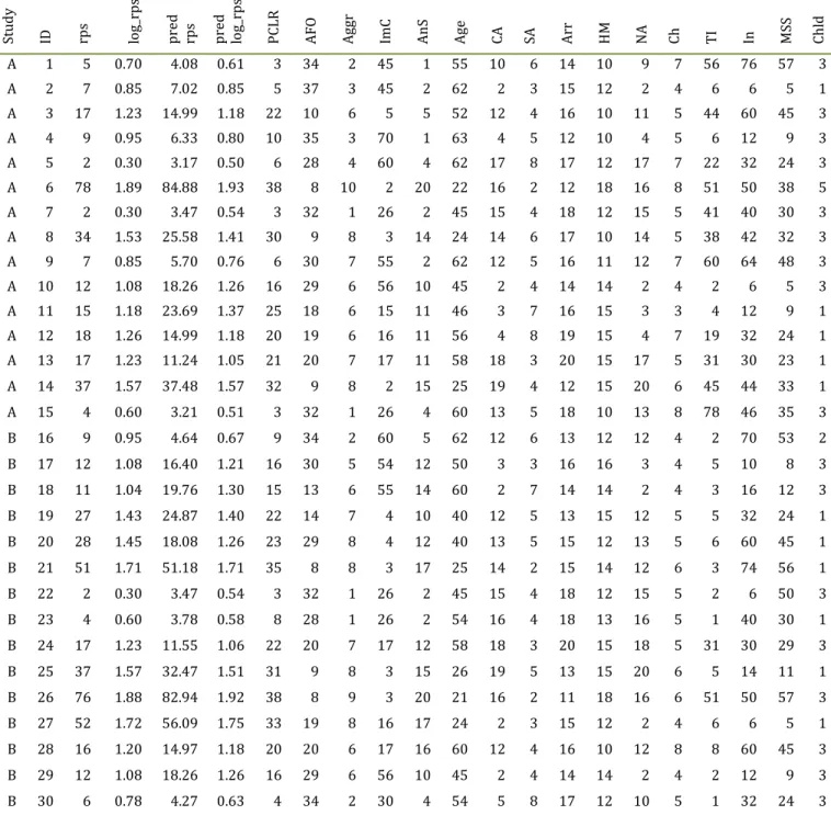
To do so, the researchers select 16 risk factors, which can be assessed by examining the offenders’ files. Examples include the offenders’ current age (Age), score on the Psychopathy Checklist Revised (PCLR; Hare, 2003), and history of substance abuse (SA). Next, the researchers select data from a random sample of 30 offenders with known RPS scores from two penitentiaries. Table 1 presents the data for each of the 30 offenders. Note that the columns with the predicted RPS scores (pred rps) and the logarithmically transformed RPS scores (pred log_rps) are generated later in this example.
Data from the offenders in penitentiary A (n = 15) are used to train the model, and those from
1
penitentiary B (n = 15) are used to test the model. Because forensic settings can pose challenges for recruitment and data collection—resulting in a smaller number of observations relative to predictors—and because the study is exploratory, the researchers decide that PLSR is the ideal prediction technique to employ. Using PLSR, the researchers aim to determine a) whether a few underlying predictive factors account for most of the variation in RPS scores, b) whether all 16 predictor variables contribute to the model, and c) whether this model can accurately predict RPS scores.
In this example, figures and outputs are generated using JMP version 10 software; references to SAS version 9.3 are made throughout. JMP is particularly useful for data exploration because of the multitude of highly informative figures that can be easily produced—several of which are demonstrated below. In JMP, PLSR can be found under the analyze tab by selecting multivariate methods and partial least squares. In SAS, PLSR is computed using the PROC PLS statement followed by a specification of the predictor and response variables in the MODEL statement. For a thorough outline of PROC PLS and the available options, see chapter 51 in the SAS/STAT User’s Guide (SAS Institute Inc., 1999).
Prior to analysis, the distributions of the predictor and response variables should be assessed. In this example, the original RPS scores are highly negatively skewed. As shown in Table 1, the RPS scores (rps) are logarithmically transformed (log_rps). All predictor variables are sufficiently normally distributed and so no transformation is performed. As previously stated, the first 15 observations are used to build the PLSR model. As such, the dataset is split into training and test sets by excluding and hiding rows 16 to 30 (i.e., rows with ID values 16 to 30).
Once the PLS statistic is selected, the predictor and response variables must be specified. This is important because the predictor variables are measured on different scales and have different means and standard deviations. Next, in the JMP Model Launch window, the type of PLSR algorithm must be specified. In this example, we are predicting a single continuous response variable and so the NIPALS and SIMPLS algorithms would produce identical prediction scores. We accept the default NIPALS (NIPALS is also the default algorithm in SAS).
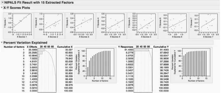
score plots are shown for the first seven factors only). In both JMP and SAS, the maximum number of factors that can be extracted for any given dataset is 15. First, we can see that the correlation between the X
predictors and the Y response is highest for the first few factors and decreases with each subsequent factor. We can also see that 100% of the variation of X and Y is explained with 14 factors. Remember, it is important to Table 1
Table 1Table 1
Table 1 Hypothetical dataset used in PLS example
S
tu
d
y
ID rps log
_r
p
s
p
re
d
rp
s
p
re
d
lo
g
_r
p
s
P
C
L
R
A
F
O
A
g
g
r
Im
C
A
n
S
A
g
e
C
A SA Arr
H
M
N
A
C
h TI
In MS
S
C
h
ld
A 1 5 0.70 4.08 0.61 3 34 2 45 1 55 10 6 14 10 9 7 56 76 57 3
A 2 7 0.85 7.02 0.85 5 37 3 45 2 62 2 3 15 12 2 4 6 6 5 1
A 3 17 1.23 14.99 1.18 22 10 6 5 5 52 12 4 16 10 11 5 44 60 45 3
A 4 9 0.95 6.33 0.80 10 35 3 70 1 63 4 5 12 10 4 5 6 12 9 3
A 5 2 0.30 3.17 0.50 6 28 4 60 4 62 17 8 17 12 17 7 22 32 24 3
A 6 78 1.89 84.88 1.93 38 8 10 2 20 22 16 2 12 18 16 8 51 50 38 5
A 7 2 0.30 3.47 0.54 3 32 1 26 2 45 15 4 18 12 15 5 41 40 30 3
A 8 34 1.53 25.58 1.41 30 9 8 3 14 24 14 6 17 10 14 5 38 42 32 3
A 9 7 0.85 5.70 0.76 6 30 7 55 2 62 12 5 16 11 12 7 60 64 48 3
A 10 12 1.08 18.26 1.26 16 29 6 56 10 45 2 4 14 14 2 4 2 6 5 3
A 11 15 1.18 23.69 1.37 25 18 6 15 11 46 3 7 16 15 3 3 4 12 9 1
A 12 18 1.26 14.99 1.18 20 19 6 16 11 56 4 8 19 15 4 7 19 32 24 1
A 13 17 1.23 11.24 1.05 21 20 7 17 11 58 18 3 20 15 17 5 31 30 23 1
A 14 37 1.57 37.48 1.57 32 9 8 2 15 25 19 4 12 15 20 6 45 44 33 1
A 15 4 0.60 3.21 0.51 3 32 1 26 4 60 13 5 18 10 13 8 78 46 35 3
B 16 9 0.95 4.64 0.67 9 34 2 60 5 62 12 6 13 12 12 4 2 70 53 2
B 17 12 1.08 16.40 1.21 16 30 5 54 12 50 3 3 16 16 3 4 5 10 8 3
B 18 11 1.04 19.76 1.30 15 13 6 55 14 60 2 7 14 14 2 4 3 16 12 3
B 19 27 1.43 24.87 1.40 22 14 7 4 10 40 12 5 13 15 12 5 5 32 24 1
B 20 28 1.45 18.08 1.26 23 29 8 4 12 40 13 5 15 12 13 5 6 60 45 1
B 21 51 1.71 51.18 1.71 35 8 8 3 17 25 14 2 15 14 12 6 3 74 56 1
B 22 2 0.30 3.47 0.54 3 32 1 26 2 45 15 4 18 12 15 5 2 6 50 3
B 23 4 0.60 3.78 0.58 8 28 1 26 2 54 16 4 18 13 16 5 1 40 30 1
B 24 17 1.23 11.55 1.06 22 20 7 17 12 58 18 3 20 15 18 5 31 30 29 3
B 25 37 1.57 32.47 1.51 31 9 8 3 15 26 19 5 13 15 20 6 5 14 11 1
B 26 76 1.88 82.94 1.92 38 8 9 3 20 21 16 2 11 18 16 6 51 50 57 3
B 27 52 1.72 56.09 1.75 33 19 8 16 17 24 2 3 15 12 2 4 6 6 5 1
B 28 16 1.20 14.97 1.18 20 20 6 17 16 60 12 4 16 10 12 8 8 60 45 3
B 29 12 1.08 18.26 1.26 16 29 6 56 10 45 2 4 14 14 2 4 2 12 9 3
B 30 6 0.78 4.27 0.63 4 34 2 30 4 54 5 8 17 12 10 5 1 32 24 3
choose the number of factors that maximizes the covariance between X and Y scores without overfitting the data.
To select the optimum number of extracted factors, we run PLSR using cross validation. The results indicate that the smallest value for the PRESS statistic is for two factors (PRESS = .53; see Figure 2). With two factors, 61% of the variation is explained for X and 88% of the variation is explained for Y.
This example will be continued using two factors; however, it should be acknowledges that the van der Voet statistic indicates that a two-factor model is not significantly different than a one-factor model. Remember, the number of factors selected by the van der Voet statistic is the smallest number of factors with residuals that are not significantly different than the residuals of the model with the smallest absolute PRESS value. While the number of extracted factors is left to the discretion of the researcher (who should consider the interpretability of the factors), the model with the fewest factors is typically preferred. In this example, the predictors tend to cluster into factors related to the offender’s personality and temperament (Factor 1), and demographics and criminal history (Factor 2). For this reason, we opt to use a two-factor prediction model.
Under the NIPALS dropdown menu in JMP, a multitude of figures and plots can be selected that are useful for data exploration. First, the overlay loading plot (see Figure 3) shows the factor loadings for each predictor variable for Factor 1 and Factor 2. This plot
helps us to visualize the relationships between the predictors and the extracted factors. Note that a similar plot is automatically produced showing the factor loadings for each response variable; this plot is not presented here because we are attempting to predict only one response variable and, therefore, the plot is uninformative. We can see that some predictors load heavily, in absolute terms, onto Factor 1 and minimally onto Factor 2, such as the variables PCLR and AFO.
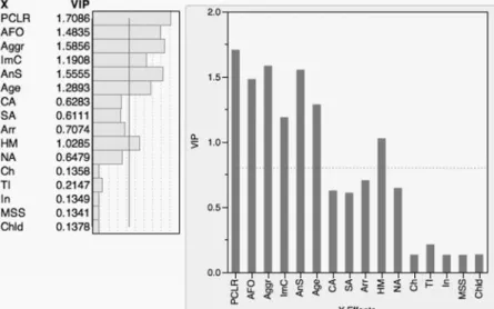
Next, we want to determine whether or not all 16 variables are important to the model or if some can be pruned. The variable importance for the projection (VIP) statistic is defined as a weighted sum of squares of the weights (Wold, 1995). The higher a variable’s VIP score, the more influential it is in determining the PLSR model for both predictors and responses. Although VIP cut-off points vary throughout the literature, traditionally variables with VIP scores lower than 0.8 are deemed as non-influential in the model. As shown in the VIP plot in Figure 4, 9 of the 16 variables have VIP lower than 0.8. For a variable to be considered for removal from the model, however, one must also look at its regression coefficient.
The VIP versus coefficient plot is shown in Figure 5. The regression coefficient represents a predictor variables’ importance in predicting the response. While JMP will produce the VIP versus coefficient plots for both the original data and the centered and scaled data, one should only consider the latter, if indeed the data were centered and scaled (Cox & Gaudard, 2013). Figure 1
Figure 1 Figure 1
Again, 9 of the 16 variables have VIP lower than the cut-off of 0.8. We can also see that the absolute values of the regression coefficients for five of these variables (MSS, TI, Chld, In, Ch) are near zero. On the other hand, four of the nine variables with low VIP (Arr, CA, SA, NA) have absolute values that are relatively high and comparable to the other variables with VIP greater than 0.8. In general, if a predictor has a VIP less than 0.8 and a small regression coefficient, it can be confidently removed from the model. For this reason, five variables with low VIP and small coefficients (MSS, TI, Chld, In, Ch) are removed from the model. We will err on the side of caution and retain the other four variables with low VIP because their coefficients indicate that they may be influential in our model. The SAS/STAT User’s Guide provides the statements necessary to generate the VIP and regression coefficients (SAS Institute Inc., 1999).
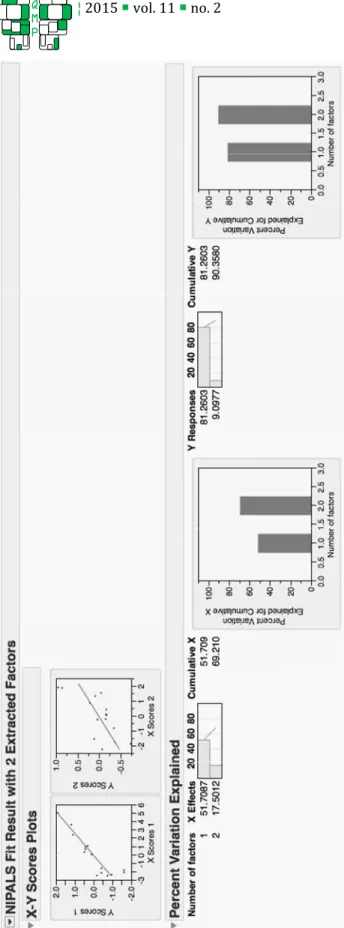
We are now going to run the pruned model using the same PLSR procedures as above while
including only 11 of the 16 predictors. With the removal of these five predictors, the two-factor model explains a greater proportion of the variance of X and Y than the one-factor model: 69% and 90%, respectively (see Figure 6). As such, the model with the reduced number of predictor variables is a better fit. The reduced model is also preferable for the researchers who wish to predict RPS scores based on a fewer number of variables.
The new prediction formula should be saved (under NIPALS options). Doing so adds a new column to the data set: the predicted response score (pred log_rps).
From this score, we generated the antilog scores (pred rps) to facilitate the comparison of the actual and predicted RPS (see Table 1). Note that the prediction score will be generated for all observations, even if the observation was excluded from the analysis. Looking at Table 1, the actual and predicted RPS scores appear to be fairly similar. For example, the actual RPS score for offender 1 (ID 1) is 5 and his predicted RPS score is 4.
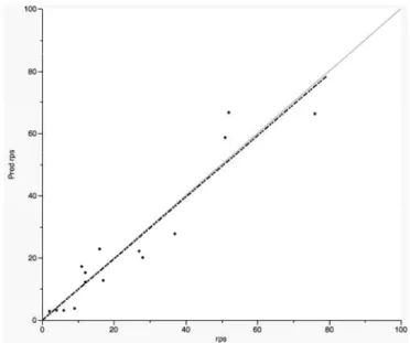
To evaluate our prediction formula, we will assess the test set. To do so, we hide and exclude the rows of the offenders from Penitentiary A and make available the rows of the offenders from Penitentiary B. A visual comparison of the actual versus predicted RPS scores allows us to visually compare the scores and gauge the accuracy of the two-factor prediction model. The JMP graph builder can be used to plot the predicted versus actual scores (pred rps vs. rps). Figure 7 shows the accuracy of the model. The dotted line is the line of Figure 2
Figure 2 Figure 2
Figure 2 PRESS and van der Voet statistics produced by cross validation (in JMP).
Figure 3 Figure 3Figure 3
Figure 3 Overlay loadings plot for the X predictors (in JMP).
Factor 1
Factor 2
Figure 4 Figure 4 Figure 4
best-fit, where a slope of 1 would indicate that the model is highly accurate at predicting the response. The
closer the data points (i.e., observations) are to the grey diagonal reference line, the more accurate the prediction formula. Also, if the prediction formula were completely accurate in predicting RPS, the line of best fit would overlap with the diagonal line. Altogether, this graph indicates that our prediction formula is fairly accurate at predicting RPS scores, particularly for lower scores where the points fall closer to the diagonal and best fit lines.
In JMP, there are several other plots that can be produced to determine the acceptability of the predictive model (e.g., diagnostic plots; see Cox & Gaudard, 2013). It is up to the researcher to decide, based on the interpretability of the data, the degree of accuracy that is acceptable. In this hypothetical example it may in fact be more important to accurately predict lower response scores than higher response scores because the accuracy of decision-making regarding parole and sentencing may be more critical for offenders with low RPS scores.
Using PLSR, we have been able to determine that indeed a subset of variables can be used to predict RPS. We now know that it would be worthwhile to attempt to replicate these findings using a larger sample of offenders. Once more data has been gathered, other prediction techniques could be employed to increase our confidence in the model and to better understand the relationships between the predictor and response variables and the underlying factors.
Conclusion Conclusion Conclusion Conclusion
The primary focus of this paper was to outline PLSR as a predictive technique through factor extraction. As discussed in our introduction, PLSR is a powerful tool for generating and testing models in complex datasets. By using regression analysis as its base, and through its distinct way of producing latent variables, PLSR can help produce generalizable models across multiple predictors and responses. We highlighted how PLSR compares to and can help overcome issues found in other statistical procedures (e.g., MLR, PCR), and finally we presented guidelines on how PLSR can be applied.
Our hypothetical example was produced using the JMP statistical software package. JMP is a powerful statistical package, designed as a more visual and interactive companion to SAS. We chose JMP precisely due to its ability to produce intuitive and informative graphical information. Wherever possible, we made reference to SAS—while providing additional references for those who are interested—because it is a Figure 5
Figure 5 Figure 5
popular and versatile statistical program.
We hope that this brief introduction to PLSR will encourage social sciences researchers to continue to learn about this technique and to discover its many uses (e.g., data exploration). As previously noted, PLS has additional nuances and variants that we did not cover. We focused on the application of PLSR to datasets with many predictors and a single response, but PLSR can also be used when the predictors and responses are multivariate. For those interested in more in-depth information, we would point to additional references (e.g., Abdi, 2007; Geladi & Kowalski, 1986; Helland, 1988; Rosipal & Krämer, 2006; Wold, Ruhe, Wold, & Dunn, 1984).
Authors’ notes and acknowledgments Authors’ notes and acknowledgments Authors’ notes and acknowledgments Authors’ notes and acknowledgments
The authors wish to acknowledge the helpful comments
provided by Dwayne Schindler.
References References References References
Abdi, H. (2007). Partial least squares regression: PLS-regression. In N. Salkind (Ed.) Encyclopedia of
Measurement and Statistics (pp. 792-795).
Thousand Oaks, CA: Sage.
Abdi, H., & Williams, L. J. (2013). Partial least squares methods: Partial least squares correlation and partial least square regression. In B. Reisfeld & A. N. Mayeno (Eds.), Computational Toxicology, Volume II, Methods in Molecular Biology (Vol. 930, pp. 549– 578). Totowa, NJ: Humana Press. doi: 10.1007/978- 1-62703-059-5
Arlot, S. & Celisse, A. (2010). A survey of cross-validation procedures for model selection. Statistics Surveys, 4, 40-79. doi: 10.1214/09-SS054
Campbell, M. J. (2006). Statistics at square two: Understanding modern statistical applications in medicine (2nd ed.). Oxford, UK: Blackwell Publishing Ltd. doi: 10.1002/9780470755839
Cox, I., & Gaudard, M. (2013). Discovering Partial Least Squares with JMP®. Cary, NC: SAS Institute Inc. Dunn Iii, W., Scott, D., & Glen, W. (1989). Principal
components analysis and partial least squares regression. Tetrahedron Computer Methodology, 2, 349-376. doi: 10.1016/0898-5529(89)90004-3 Geladi, P., & Kowalski, B. R. (1986). Partial
least-squares regression: A tutorial. Analytica Chimica
Acta, 185, 1-17. doi:
10.1016/0003-2670(86)80028-9
Geladi, P., & Esbensen, K. (1991). Regression on multivariate images: principal component regression for modeling, prediction and visual diagnostic tools. Journal of Chemometrics, 5, 97-111. doi: 10.1002/cem.1180050206
Haenlein, M., & Kaplan, A. M. (2004). A beginner’s guide Figure 6
Figure 6Figure 6
Figure 6 VIP versus coefficient plot for the centered and scaled data (in JMP).
Figure 7 Figure 7 Figure 7
Figure 7 Comparison of the predicted versus the actual RPS scores for the test set. The dotted line represents the line of best fit while the grey is a reference line plotted at the diagonal.
to partial least squares analysis. Understanding
Statistics, 3, 283-297. doi: 10.1207/
s15328031us0304_4
Hare, R. D. (2003). Manual for the Revised Psychopathy Checklist (2nd ed.). Toronto: Multi-Health Systems. Helland, I. S. (1988). On the structure of partial least
squares regression. Communications in Statistics-Simulation and Computation, 17, 581-607. doi: 10.1080/03610918808812681
Hox, J. J., & Bechger, T. M. (1998). An introduction to structural equation modeling. Family Science Review, 11, 354-373.
Huang, J., & Harrington, D. (2005). Iterative partial least squares with right censored data analysis: A comparison to other dimension reduction techniques. Biometrics, 61, 17-24. doi: 10.1111/j.0006-341X.2005.040304.x
Mason, C. H., & Perreault Jr, W. D. (1991). Collinearity, power, and interpretation of multiple regression analysis. Journal of Marketing Research, 28(3), 268-280. doi: 10.2307/3172863
Reinartz, W., Haenlein, M., & Henseler, J. (2009). An empirical comparison of the efficacy of covariance-based and variance-covariance-based SEM. International Journal of Research in Marketing, 26(4), 332-344. doi: 10.1016/j.ijresmar.2009.08.001
Rosipal, R., & Krämer, N. (2006). Overview and recent advances in Partial Least Squares. In C. Saunders, M. Grobelnik, S. Gunn & J. Shawe-Taylor (Eds.), Subspace, Latent Structure and Feature Selection (pp. 34-51). Berlin, Germany: Springer.
SAS Institute Inc. (1999). The PLS procedure. SAS/STAT® User’s Guide Version 8 (pp. 2693-2732). Cary, NC: SAS Institute Inc.
Sutter, J. M., Kalivas, J. H., & Lang, P. M. (1992). Which principal components to utilize for principal component regression. Journal of Chemometrics,
6(4), 217-225. doi: 10.1002/cem.1180060406 Tenenhaus, M., Vinzi, V. E., Chatelin, Y.-M., & Lauro, C.
(2005). PLS path modeling. Computational Statistics
& Data Analysis, 48(1), 159-205. doi:
10.1016/j.csda.2004.03.005
Tobias, R. (1995). An introduction to partial least squares regression.Proceedings of the Twentieth Annual SAS Users Group International Conference. Cary, NC: SAS Institute Inc.
Van Roon, P., Zakizadeh, J., & Chartier, S. (2014). Partial least squares tutorial for analyzing neuroimaging data. The Quantitative Methods for Psychology, 10, 200-215.
Vinzi, V. E., & Lauro, C. (Eds.). (2005). Partial least squares [Special issue]. Computational Statistics & Data Analysis, 48(1).
Wentzell, P. D., & Vega Montoto, L. (2003). Comparison of principal components regression and partial least squares regression through generic simulations of complex mixtures. Chemometrics and Intelligent
Laboratory Systems, 65, 257-279. doi:
10.1016/S0169-7439(02)00138-7
Wold, H. (1975). Soft modeling by latent variables: The nonlinear iterative partial least squares approach. In J. Gani (Ed.), Perspectives in Probability and Statistics, Papers in Honour of M. S. Bartlett (pp. 520-540). London, UK: Academic Press.
Wold, S. (1995). PLS for multivariate linear modeling. In H. van der Waterbeemd (Ed.), Chemometric
Methods in Molecular Design (pp. 195-218).
Weinheim, Germany: VCH Publishers.
Wold, S., Ruhe, A., Wold, H., & Dunn, I., WJ. (1984). The collinearity problem in linear regression. The partial least squares (PLS) approach to generalized inverses. SIAM Journal on Scientific and Statistical Computing, 5, 735-743. doi: 10.1137/0905052
Citation Citation Citation Citation
Sawatsky, M. L., Clyde, M., & Meek, F. (2015). Partial least squares regression in the social sciences. The Quantitative Methods for Psychology, 11 (2), 52-62.
Copyright © 2015 Sawatsky, Clyde & Meek. This is an open-access article distributed under the terms of the Creative Commons Attribution License (CC BY). The use, distribution or reproduction in other forums is permitted, provided the original author(s) or licensor are credited and that the original publication in this journal is cited, in accordance with accepted academic practice. No use, distribution or reproduction is permitted which does not comply with these terms.