Structure and genetic relationships between Brazilian naturalized and exotic
purebred goat domestic goat (
Capra hircus
) breeds based on microsatellites
Joelliton Domingos de Oliveira
1,2, Maria Luiza Silveira de Paiva Igarashi
1,3,
Théa Mírian Medeiros Machado
4, Marcos Mateo Miretti
3*, Jesus Aparecido Ferro
3and Eucleia Primo Betioli Contel
11
Departamento de Genética, Faculdade de Medicina, Universidade de São Paulo, Ribeirão Preto,
SP, Brazil.
2
Universidade Estadual do Mato Grosso do Sul, Dourados, MS, Brazil.
3
Departamento de Tecnologia, Faculdade de Ciências Agrárias e Veterinária,
Universidade Estadual Paulista, Jaboticabal, SP, Brazil.
4
Departamento de Zootecnia, Universidade Federal de Viçosa, Viçosa, MG, Brazil.
Abstract
The genetic relationships and structure of fourteen goat (Capra hircus) populations were estimated based on geno-typing data from 14 goat populations (n = 410 goats) at 13 microsatellite loci. We used analysis of molecular variance (AMOVA), principal component analysis (PCA) and F statistics (FIS, FITand FST) to evaluate the genetic diversity (Ho,
He and ad) of the goats. Genetic distances between the 14 goat populations were calculated from allelic frequency data for the 13 microsatellite markers. Moderate differentiation was observed for the populations of the undefined breeds (including the Anglo-Nubian-M breed), the naturalized Brazilian breeds (Moxotó, Canindé), the exotic pure-bred breeds (Alpine, Saanen, Toggenbourg and Anglo-Nubian) and the naturalized Brazilian Graúna group. Our AMOVA showed that a major portion (88.51%) of the total genetic variation resulted from differences between indi-vidual goats within populations, while between-populations variation accounted for the remaining 11.49% of genetic variation. We used a Reynolds genetic distance matrix and PCA to produce a phenogram based on the 14 goat pop-ulations and found three clusters, or groups, consisting of the goats belonging to the undefined breed, the naturalized breeds and the exotic purebred breeds. The closer proximity of the Canindé breed from the Brazilian state of Paraíba to the Graúna breed from the same state than to the genetically conserved Canindé breed from the Brazilian state of Ceará, as well as the heterozygosity values and significant deviations from Hardy-Weinberg equilibrium suggests that there was a high number of homozygotes in the populations studied, and indicates the importance of the State for the conservation of the local breeds. Cataloguing the genetic profile of Brazilian goat populations provides essen-tial information for conservation and genetic improvements programs.
Key words:goat, microsatellite, genetic distance, PCA, AMOVA, genetic relationships, genetic diversity, F statistics. Received: April 7, 2006; Accepted: September 28, 2006.
Introduction
Microsatellite polymorphisms have proved to be a useful tool for the analysis of genetic structure and the ge-netic divergence between populations and is also important for verifying pedigree relationships and providing funda-mental information for the preservation of breeds.
Compared with other farm animals, few studies have been conducted using microsatellite markers to investigate genetic distance in domesticated goats(Capra hircus)
(Saitbekovaet al., 1999; Yanget al., 1999; Barkeret al.
2001; Kimet al., 2002 ; Liet al., 2002; Baumunget al.,
2004). In Brazil, caprine breeds have been studied using morphological characters (Machadoet al., 2000), protein
markers (Igarashiet al., 2000) and random amplified
poly-morphic DNA (RAPD) markers (Oliveiraet al., 2005).
According to the Brazilian Geographic and Statistics Foundation (Instituto Brasileiro de Geografia e Estatística -IBGE), the vast majority of Brazilian goats (93%) are lo-cated in the northeastern region of Brazil where two groups can be identified, naturalized goats and goats of undefined breed. The naturalized goats tend to be small and highly heterogeneous, especially for coat colors. There are four major breeds, Moxotó, Canindé, Repartida and Marota, along with the Graúna group formed by goats with black
www.sbg.org.br
Send correspondence to Joelliton Domingos de Oliveira. Departa-mento de Genética, Faculdade de Medicina, Ribeirão Preto, SP, Brazil. E-mail: oliveira.jd@ig.com.br.
*Present address: Wellcome Trust Sanger Institute, Hinxton, Cam-bridge, United Kingdom CB10 1SA.
coat color (Santos, 1987) but which has not yet been re-garded as a Brazilian breed by the Brazilian Goat Breeders Association (Associação Brasileira de Criadores de Capri-nos – ABCC) because this association requires other stan-dardized characteristics in addition to coat color. The goats of undefined breed (UDB) constitute the largest group in the Brazilian northeast, and includes all goats that cannot be assigned to any other breed. This group comprises goats with diverse coat color patterns as well as various degrees of crossing with exotic purebred goats such as those of the Toggenbourg, Anglo-Nubian, Alpine and Saanen breeds, such crossings having been made to improve milk and meat production (KP Pant, personal communication). The cross-ing of diverse breads interferes with genetic conservation programs for naturalized and UDB breeds and affects the genetic structure and relationships among the breeds. As-sessing the genetic composition of Brazilian naturalized, UDB and exotic purebred goats is important for determin-ing the current genetic structure of these populations and would provide substantial information for genetic improve-ment and conservation programs. The objective of the pres-ent study was to investigate the genetic structures of 14 goat populations and to analyze the genetic relationship between them using 13 microsatellite markers. We included the Graúna group in our investigation to compare our results with those reported by Igarashiet al.(2000). To increase
the understanding about the diversity of these goat popula-tions we also compared our results to those of Araújoet al
(2006) who also used microsatellite loci to investigate the genetic diversity between Alpine, Saanen and Moxotó goats.
Material and Methods
DNA extraction and amplification conditions
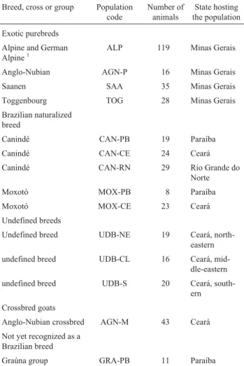
A total of 410 goats (Capra hircus) from a blood sam-ple collection previously obtained by Igarashiet al.(2000) was used (Table 1).
We extracted DNA from 300µL of goat blood
ac-cording to the method of Higuchi (1989) with some modi-fications. Amplification reactions were done in a TGradient (Biometra, Germany) thermocycler in a final reaction volume of 15µL containing 0.2-0.5 µg of
tem-plate DNA, 0.1 mM of each dNTP, 0.5 U of Taq DNA polymerase (Life Technologies, EUA), 1X reaction buffer (50 mM KCl, 2 mM MgCl2, 20 mM Tris-HCl, pH 8.4) and 10 pmol of primers. A two-stage touchdown amplification program was designed for DNA amplification. An initial denaturation step of 4 min at 94 °C was used in all pro-grams, followed by amplification cycles in which the an-nealing temperature (Tm) was gradually decreased by 1 °C every amplification cycle. This treatment was fol-lowed by a second stage consisting of either 28 or 30 am-plification cycles, in which the Tm remained constant. Denaturation and elongation steps were held constant for
45 s at 94 °C and 72 °C, respectively, during both stages. An elongation step of 10 min at 72 °C was performed in all programs after stage 2. The 13 microsatellite markers se-lected for assessing genetic diversity in the goat popula-tions described in Table 1 were: INRA011, INRA040, BM3517, ILST030, ILST028, UWCA46, TEXAN02, ILST011, INRA023, SRCRSP9, MHCIIDR, INRA006 and IDVGA37. These markers were originally described in cattle, with the exception of the caprine SRCRSP9 markers. One PCR primer from each pair was labeled with an appropriate dye, 6FAM, HEX or NED (PE Biosystems, USA) and the polymerase chain reactions (PCR) were car-ried out as described above resulting in strong and specific PCR products which were analyzed in an ABI PRISM 377 automatic DNA sequencer using standard loading condi-tions and a 2 h electrophoresis run on 5% (w/v) Long Ranger gel. Alleles were sized relative to a ROX GS 500 internal size standard (Applied Biosystems, USA) and an-alyzed with the Applied Biosystems GENESCAN pro-gram version 2.1. Size estimates, in base pairs (bp), were manually checked for genotyping errors.
Table 1- List of the goat populations studied.
Breed, cross or group Population code Number of animals State hosting the population Exotic purebreds Alpine and German
Alpine1 ALP 119 Minas Gerais
Anglo-Nubian AGN-P 16 Minas Gerais
Saanen SAA 35 Minas Gerais
Toggenbourg TOG 28 Minas Gerais
Brazilian naturalized breed
Canindé CAN-PB 19 Paraíba
Canindé CAN-CE 24 Ceará
Canindé CAN-RN 29 Rio Grande do
Norte
Moxotó MOX-PB 8 Paraíba
Moxotó MOX-CE 23 Ceará
Undefined breeds
Undefined breed UDB-NE 19 Ceará,
north-eastern
undefined breed UDB-CL 16 Ceará,
mid-dle-eastern
undefined breed UDB-S 20 Ceará,
south-ern Crossbred goats
Anglo-Nubian crossbred AGN-M 43 Ceará Not yet recognized as a
Brazilian breed
Graúna group GRA-PB 11 Paraíba
1German Alpine and the Alpine breed animals were grouped together due
Data analysis
Allelic frequencies, observed heterozygosity (Ho), expected heterozygosity (He) and exact tests of genotypic frequencies for deviation from Hardy-Weinberg equilib-rium (HWE) were carried out using the GENEPOP v.3.4 program (Raymond and Rousset, 1995). The exact test of Hardy-Weinberg proportion for multiple alleles (Guo and Thompson, 1992) was performed using the Markov chain procedure (1,000 batches, 5,000 iterations, 10,000 de-me-morization steps). The number of private alleles and allelic diversity were assessed using the FSTAT program v.2.9.3 (Goudet, 2001). A principal component analysis (PCA) was performed on the populations using the PCAGEN pro-gram (J.Goudet, unpublished). Populations were ordered according to the first and second PCA axes. The signifi-cance of each principal component was assessed from 5,000 randomizations. The F-Statistics (Wright, 1951) were calculated by the method of Weir and Cockerham (1984) using the GDA program (Lewis and Zaykin, 1997) and the significance of the F values were estimated from 10,000 replicates by bootstrapping, with confidence inter-vals not including zero being considered significantly dif-ferent from zero.
The groups obtained from the PCA analyses were subjected to analysis of molecular variance (AMOVA; Excoffieret al., 1992) using the ARLEQUIN 3.0 program
(Excoffieret al., 2005). Significance was determined from
10,000 permutations. Reynolds distances (Reynoldset al.,
1983) between populations were generated from allelic fre-quency data using the PHYLIP package, v.3.65 (Felsens-tein, 2005). Genetic distances were calculated using the GENDIST program and used to construct a Neighbor-Joining (NJ) tree in the NEIGHBOR program. To test the robustness of tree topologies, 1,000 bootstrap replicates of the allele frequency file were generated in the SEQBOOT program and analyzed using GENDIST. Tree topologies were created for all replicates using NEIGHBOR and a consensus tree was generated by the CONSENSE program. These programs are incorporated in the PHYLIP package, v.3.65 (Felsenstein, 2005).
Results
Genetic diversity within and between populations
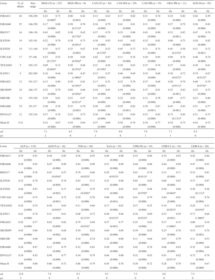
All 13 loci were polymorphic, showing an average of 15.6 alleles per locus (min = 9, max = 26 alleles; Table 2). Allelic diversity was lowest for the MOX-PB (4.5) popula-tion and highest for ALP (12.8) populapopula-tion. The meanHo
value varied from 0.28 to 0.46 andHefrom 0.64 to 0.80. The MOX-PB population was the least variable (He = 0.64), while the ALP (He = 0.80) and TOG (He= 0.79) populations showing the highestHevalues. In a total of 203 alleles we detected 10 private alleles (5%) over all the populations (Table 2) and the average private allele frequency was 0.075 (min = 0.004, max = 0.0425).
We detected 38 non-significant deviations from HWE from a total of 182 loci/population (p > 0.01). In con-trast, the remaining loci/populations (144) showed Hardy-Weinberg disequilibrium (p < 0.01; Table 2). The populations presenting loci with no significant deviations were: MOX-C (UWCA46, TEXAN02); MOX-PB (INRA040, BM3517, ILST030, UWCA46, TEXAN02, ILST011, INRA023, SRCRSP9, MHCIIR); CAN-CE (ILST028, TEXAN02); GRA-PB (ILST028, ILST011, INRA023, IDVGA37); AGN-M (ILST011, INRA023); AGN-P (BM3517, TEXAN02); TOG (BM3517, ILST028, ILST011, INRA023); SAA (BM3517, ILST011); UDB-NE (BM3517, ILST028, ILST011); UDB-CL (ILST028, TEXAN02, INRA023, IDVGA37); UDB-S (ILST028, TEXAN02, ILST011, INRA023). When either all populations or all loci were pooled, significant differ-ences between Ho and He (p < 0.001) were detected
(Table 2). Allele frequencies are available as supplemen-tary material (Table S1).
Genetic differentiation and PCA
The pattern of genetic differentiation was represented by a plot of scores based on allelic frequency from 14 goat populations (Figure 1). The first principal component axis (PC1) accounted for 32.72% (p = 0.000) of the total genetic diversity, and the second (PC2), for 13.72% (p = 0.056, not significant). The PCA plot gives the position of the popula-tions according to either their known or apparent origins (historical data; Igarashiet al., 2000). The PC1 axis repre-sents the differentiation between exotic purebred popula-tions (AGN-P, SAA, TOG and ALP) and native and UDB populations (MOX-CE, MOX-PB, CAN-CE, CAN-RN, CAN-PB, GRA-PB, AGN-M, UDB-NE, UDB-CL and UDB-S) whereas the PC2 axis, although not significant, ap-parently distinguishes native and UDB populations. From this, a primary structuring suggested three major groupings of populations: (1) AGN-P, SAA, TOG and ALP, (2) MOX-CE, MOX-PB, CAN-CE, CAN-RN, CAN-PB and GRA-PB, and (3) AGN-M, UDB-NE, UDB-CL and UDB-S.
Genetic relationship
Table 2- Summary of observed (Ho), expected (He), mean (H) heterozygosity, allelic diversity (ad) and number of private alleles (pa) over all goat popu-lations. At the single-population single-locus levels a total of 38 non-significant deviations from HWE were detected. Significant deviations from HWE were detected when either all populations or all loci were pooled (p < 0.001). * = no significant difference betweenHo eHe(p > 0.01).
Lócus N. of
alleles rangeSize MOX-CE (n = 23)
a
MOX-PB (n = 8) CAN-CE (n = 24) CAN-RN (n = 29) CAN-PB (n = 19) GRA-PB (n = 11) AGN-M (n = 43)
Ho He Ho He Ho He Ho He Ho He Ho He Ho He
INRA011 26 196-250 0.22 0.73 0.00 0.41 0.13 0.63 0.17 0.82 0.21 0.74 0.18 0.82 0.26 0.59 (0.000)b (0.005) (0.000) (0.000) (0.000) (0.000) (0.000)
INRA040 25 166-258 0.17 0.80 0.50 0.70 0.26 0.79 0.41 0.81 0.31 0.82 0.27 0.79 0.26 0.83 (0.000) (0.212)* (0.000) (0.000) (0.000) (0.000) (0.000) BM3517 14 100-138 0.45 0.82 0.50 0.62 0.57 0.79 0.35 0.88 0.43 0.89 0.33 0.82 0.47 0.74
(0.000) (0.378)* (0.006) (0.000) (0.000) (0.001) (0.000) ILST030 14 142-181 0.22 0.79 0.38 0.73 0.38 0.83 0.43 0.82 0.32 0.81 0.09 0.73 0.58 0.82
(0.000) (0.041)* (0.000) (0.000) (0.000) (0.000) (0.000) ILST028 14 111-164 0.35 0.57 0.25 0.67 0.58 0.53 0.45 0.73 0.31 0.75 0.45 0.50 0.51 0.72
(0.000) (0.002) (0.319)* (0.000) (0.000) (0.232)* (0.001) UWCA46 17 97-140 0.52 0.55 0.50 0.69 0.42 0.87 0.11 0.76 0.29 0.85 0.09 0.76 0.40 0.74
(0.123)* (0.036)* (0.000) (0.000) (0.000) (0.000) (0.000) TEXAN02 9 105-133 0.09 0.12 0.50 0.68 0.21 0.26 0.28 0.62 0.37 0.74 0.27 0.64 0.30 0.61
(0.068)* (0.393)* (0.198)* (0.000) (0.000) (0.009) (0.000) ILST011 9 262-284 0.18 0.64 0.50 0.47 0.33 0.57 0.46 0.69 0.35 0.68 0.38 0.72 0.74 0.67
(0.000) (1.000)* (0.003) (0.000) (0.000) (0.027)* (0.012)* INRA023 12 191-217 0.13 0.49 0.38 0.41 0.17 0.31 0.32 0.74 0.37 0.68 0.50 0.74 0.60 0.74
(0.000) (0.385)* (0.005) (0.000) (0.000) (0.011)* (0.074)* SRCRSP9 18 106-137 0.52 0.79 0.88 0.84 0.54 0.85 0.59 0.84 0.37 0.81 0.55 0.82 0.23 0.75
(0.000) (0.450)* (0.000) (0.000) (0.000) (0.001) (0.000) MHCIIR 14 193-228 0.39 0.81 0.25 0.57 0.21 0.80 0.22 0.82 0.13 0.78 0.09 0.77 0.23 0.80
(0.000) (0.021)* (0.000) (0.000) (0.000) (0.000) (0.000) INRA006 19 95-137 0.30 0.78 0.25 0.74 0.58 0.89 0.59 0.82 0.39 0.67 0.45 0.83 0.51 0.77
(0.000) (0.003) (0.000) (0.001) (0.001) (0.001) (0.000) IDVGA37 12 192-216 0.57 0.78 0.25 0.73 0.38 0.86 0.52 0.85 0.53 0.82 0.73 0.85 0.51 0.75
(0.000) (0.000) (0.000) (0.000) (0.000) (0.131)* (0.000) Mean H 15.6 0.32 0.67 0.39 0.64 0.37 0.69 0.38 0.78 0.34 0.77 0.34 0.75 0.43 0.73
(0.000) (0.000) (0.000) (0.000) (0.000) (0.000) (0.000)
ad 7.1 4.5 7.9 9.0 7.8 7.1 9.3
pa 2 0 1 0 1 1 0
Locus ALP (n = 119) AGN-P (n = 16) TOG (n = 28) SAA (n = 35) UDB-NE (n = 19) UDB-CL (n = 16) UDB-S (n = 20)
Ho He Ho He Ho He Ho He Ho He Ho He Ho He
INRA011 0.39 0.91 0.44 0.85 0.36 0.92 0.49 0.90 0.53 0.86 0.19 0.83 0.42 0.84 (0.000) (0.000) (0.000) (0.000) (0.000) (0.000) (0.000) INRA040 0.29 0.92 0.47 0.89 0.43 0.90 0.51 0.89 0.44 0.88 0.44 0.89 0.47 0.91
(0.000) (0.000) (0.000) (0.000) (0.000) (0.000) (0.000) BM3517 0.48 0.76 0.47 0.57 0.79 0.86 0.58 0.69 0.41 0.74 0.13 0.71 0.35 0.81
(0.000) (0.056)* (0.035)* (0.033)* (0.011)* (0.000) (0.000) ILST030 0.22 0.79 0.56 0.74 0.43 0.71 0.23 0.80 0.05 0.82 0.06 0.83 0.37 0.87
(0.000) (0.009) (0.000) (0.000) (0.000) (0.000) (0.000) ILST028 0.66 0.87 0.63 0.71 0.64 0.79 0.51 0.83 0.41 0.48 0.50 0.68 0.50 0.56
(0.000) (0.003) (0.020)* (0.000) (0.070)* (0.044)* (0.111)* UWCA46 0.43 0.75 0.44 0.72 0.29 0.78 0.60 0.84 0.41 0.79 0.44 0.81 0.42 0.74
(0.000) (0.001) (0.000) (0.001) (0.000) (0.000) (0.000) TEXAN02 0.36 0.74 0.50 0.65 0.11 0.60 0.17 0.62 0.37 0.55 0.19 0.38 0.26 0.31
(0.000) (0.045)* (0.000) (0.000) (0.004) (0.025)* (0.034)* ILST011 0.61 0.74 0.31 0.61 0.68 0.73 0.49 0.66 0.36 0.60 0.33 0.59 0.71 0.66
(0.000) (0.004) (0.313)* (0.015)* (0.053)* (0.001) (1.000)* INRA023 0.42 0.77 0.63 0.82 0.79 0.84 0.57 0.77 0.25 0.62 0.17 0.15 0.00 0.10
(0.000) (0.009) (0.018)* (0.001) (0.000) (1.000)* (0.027)* SRCRSP9 0.42 0.86 0.38 0.68 0.39 0.82 0.60 0.88 0.39 0.83 0.25 0.76 0.55 0.76
(0.000) (0.002) (0.000) (0.000) (0.000) (0.000) (0.002) MHCIIR 0.09 0.60 0.06 0.64 0.18 0.74 0.26 0.60 0.11 0.64 0.07 0.79 0.11 0.53
(0.000) (0.000) (0.000) (0.000) (0.000) (0.000) (0.000) INRA006 0.26 0.87 0.13 0.79 0.32 0.83 0.20 0.83 0.42 0.76 0.06 0.83 0.35 0.84
(0.000) (0.000) (0.000) (0.000) (0.000) (0.000) (0.000) IDVGA37 0.54 0.83 0.94 0.77 0.54 0.79 0.66 0.80 0.32 0.83 0.81 0.82 0.75 0.78
(0.000) (0.000) (0.000) (0.000) (0.000) (0.071)* (0.000) Mean H 0.40 0.80 0.46 0.73 0.46 0.79 0.45 0.78 0.34 0.72 0.28 0.70 0.40 0.67
(0.000) (0.000) (0.000) (0.000) (0.000) (0.000) (0.000)
ad 12.8 7.4 9.5 9.3 7.3 6.8 7.5
We verified the undefined position of AGN-M and confirmed it similarity to the UDB goats by calculating the FST values from AGN-M grouped with either the UDB goats or the exotic purebreds. In the first case, the FSTvalue was lower and significant (unpublished data), so we grouped the AGN-M population with the UDB goats for the F-statistics analysis. The F-values (FISand FST) were signif-icant for all populations and groupings (UDB, native and exotic breeds; p < 0.01) and the FISvalues were high and
positive for all the populations while the FSTvalue (0.105) was moderate (Table 3). When the F-values were estimated by grouping according to historical data, the values did not change considerably, the FISmean values being high and
Figure 1- Plot of scores of principal component analysis based on allele frequency of 14 populations of goats. 1: Moxotó Ceará (MOX-C); 2: Moxotó Paraíba (MOX-PB); 3: Canindé Ceará (CAN-CE); 4: Canindé Rio Grande do Norte (CAN-RN); 5: Canindé Paraíba (CAN-PB); 6: Graúna Paraíba (GRA-PB); 7: In absorbent crossing with Anglo-Nubian purebred (AGN-M); 8: Alpine and German Alpine (ALP); 9: Anglo-Nubian (AGN-P); 10: Toggenbourg (TOG); 11: Saanen (SAA): 12: northeastern undefined breed (UDB-NE); 13: middle-eastern undefined breed (UDB-CL); 14: southern undefined breed (UDB-S).
Table 3- Estimates of FISand FSTcalculated by method of Weir and Cockerham (1984) based on allelic frequency of 14 goat populations, using the GDA program.
Locus Only UDB
FIS
Only native FIS
Only exotic purebred FIS
FISto all the populations
Only UDB FST
Only native FST
Only exotic purebred FST
FSTto all the populations
INRA011 0.567 0.778 0.555 0.620 0.112 0.033 0.031 0.110
INRA040 0.590 0.632 0.602 0.611 0.023 0.003 0.022 0.040
BM3517 0.515 0.480 0.288 0.401 0.044 0.013 0.107 0.095
ILST030 0.592 0.619 0.647 0.639 0.051 0.039 0.074 0.085
ILST028 0.258 0.350 0.262 0.288 0.054 0.243 0.054 0.152
UWCA46 0.477 0.597 0.433 0.491 0.115 0.154 0.080 0.147
TEXAN02 0.443 0.479 0.568 0.535 0.075 0.206 0.052 0.142
ILST011 0.083 0.468 0.211 0.239 0.096 0.061 0.048 0.115
INRA023 0.316 0.524 0.352 0.395 0.179 0.052 0.053 0.125
SRCRSP9 0.584 0.364 0.481 0.471 0.048 0.074 0.080 0.075
MHCIIDR 0.790 0.719 0.796 0.765 0.121 0.044 0.197 0.130
INRA006 0.525 0.444 0.714 0.587 0.073 0.078 0.067 0.093
IDVGA37 0.287 0.413 0.281 0.339 0.053 0.041 0.047 0.073
All loci 0.476 0.531 0.475 0.494 0.078 0.079 0.069 0.105
positive while the FST mean values were moderate (Table 3).
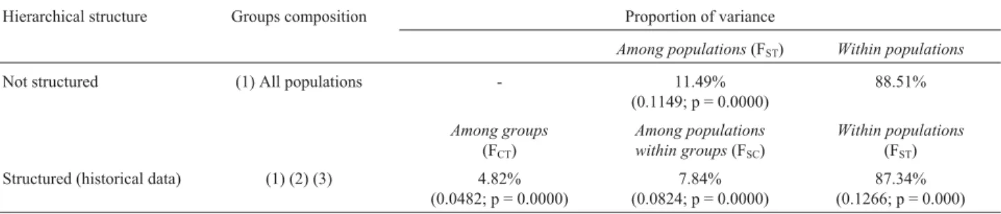
The AMOVA results for the goat populations without any structuring revealed that most of the total variation oc-curred within populations (88.51%; Table 4). The remain-der variation (11.49%) was significantly different from zero (FST= 0.1149; p < 0.01) and resulted from differences among populations. When populations were structured ac-cording to historical data, most of the total variation was observed within populations (87.34%). The remaining per-centages of variation (4.82% and 7.84%) were significantly different from zero and were attributed to differences among groups (FCT= 0.0482; p < 0.01) and among popula-tions within groups (FSC= 0.0824; p < 0.01) respectively (Table 4).
Discussion
Heterozygosity values and significant deviations from HWE suggest a large number of homozygotes in the populations studied. Deviations from HWE at microsatelli-tes loci have been reported in various studies and indicate departure from random mating (Luikartet al.; 1999; Laval et al., 2000; Barkeret al., 2001). This deviation might be
the result of inbreeding, but could also have been caused by the presence of null or non-amplified alleles, allele group-ing defects, a samplgroup-ing structure effect or selection against heterozygotes. Araújoet al.(2006) used the INRA006 and
ILST011 markers to study the Alpine, Saanen and Moxotó breeds but did not detect any deviations from HWE. This fact could be due to differences in the frequency, number and type of alleles founded in the two investigations, possi-bly due to a sampling effect. Comparing the remaining loci for the same populations, most of the loci revealed no heterozygote deficit or excess in the study of Araújoet al.
(2006) but our data indicated a deficit of heterozygotes. We believe that this divergence could have occurred because the remaining loci compared for the same breeds were ferent in the two studies, suggesting that the choice of dif-ferent loci can produce difdif-ferent results.
Populations were subjected to PCA for primary struc-turing, which resulted in a pattern of three major groups
(Figure 1), which is consistent with historical data and the neighbor-joining phenogram. This structuring is compara-ble to that reported by Igarashiet al.(2000) when the same
populations were studied with protein markers.
The F-statistics analysis was performed based on es-tablished structuring from both analyses and historical data. The FISstatistic is a measure of the extent of genetic in-breeding within subpopulations and can range from –1.0 (all individuals heterozygous) to +1.0 (no observed hetero-zygotes), while FITis a measure of the mean reduction in heterozygosity of an individual relative to the total popula-tion (Wright, 1951; Weir and Cockerham, 1984). The FIS values detected for either all the populations or for the three groups (UDB, naturalized and exotic purebred) ranged from 0.475 to 0.531 and were high and significant (p < 0.01). This indicates an excess of homozygotes due to a high level of inbreeding in the populations. However, Araújoet al.(2006) reported a different FISvalue (0.0252) when they assessed the Alpine, Saanen and Moxotó breeds. This divergence in results may be understood if we con-sider that most of the loci analyzed in the two investigations were different.
The FSTvalue measures the degree of genetic differ-entiation between populations. Considering the interpreta-tion of FST, it can be presumed that a value lying in the range 0 to 0.05 indicates little genetic differentiation, 0.05 to 0.15 indicates moderate differentiation, 0.15 to 0.25 a large degree of differentiation and values above 0.25 very great differentiation (Wright 1978; Hartl and Clark, 1997). The FSTvalues identified for either all the populations or for the three groups fell in the range 0.05 to 0.15, indicating moderate genetic differentiation for both conditions. The FSTvalue of 0.105 for all populations indicates that 10.5% of the total variability resulted from genetic differences be-tween the populations while the remaining 89.5% was due to the high diversity between individuals within each popu-lation.
The AMOVA results without subgroups definition, or when considered a hierarchical structure, revealed ge-netic differentiation between the 14 populations. When the populations were unstructured the AMOVA FSCvalue was 0.1149 (Table 4), indicating that 11.49% of the total
varia-Table 4- AMOVA results for 14 populations of goats based on FSTpairwise distance values using ARLEQUIN program. Populations were assigned according to historical data into three groups: (1) AGN-P, SAA, TOG and ALP; (2) MOX-CE, MOX-PB, CAN-CE, CAN-RN, CAN-PB and GRA-PB; (3) AGN-M, UDB-NE, UDB-CL and UDB-S.
Hierarchical structure Groups composition Proportion of variance
Among populations(FST) Within populations
Not structured (1) All populations - 11.49%
(0.1149; p = 0.0000)
88.51%
Among groups
(FCT)
Among populations within groups(FSC)
Within populations
(FST) Structured (historical data) (1) (2) (3) 4.82%
(0.0482; p = 0.0000)
7.84% (0.0824; p = 0.0000)
tion could be attributed to differences between populations. This represents a moderate difference between populations and validates the FST value detected for all populations. When populations were structured according to historical data, the AMOVA confirmed that most (87.34%) of the to-tal variation was caused by differences between individual animals within populations. The differentiation between populations within groups was higher than the differentia-tion between groups (Table 4), indicating that the UDB, naturalized or exotic purebred populations were highly dif-ferentiated.
The structuring seen in the phenogram confirmed the expected relationship of the populations (Figure 2). Iga-rashiet al.(2000) investigated these populations with
pro-tein markers and reported similar structuring. The grouping of the UDB populations with the exotic purebred popula-tions can be explained by some crossbreeding (Igarashi
et al., 2000). Native and exotic breeds, including the
An-glo-Nubian, may influence UDB populations, especially the UDB-NE and UDB-CL populations (Machadoet al.,
2000).
The branching pattern within the three major groups also showed considerable similarity to the results described by Igarashiet al.(2000), the similarities being as follows: As expected, the UDB populations were grouped in the same branch since they indirectly belong to the same group; the MOX-CE and CAN-CE populations were grouped in a separate branch, either due to the fact that they are Brazilian naturalized breeds or due to a derivative process through the isolation of the local population (Igarashiet al., 2000). According to Silva Neto (1950) the Moxotó breed may have already been brought from Portugal to Brazil in a stan-dardized form; A branch with the TOG, ALP and SAA ex-otic purebred populations occurred. In this branch, the TOG population was set apart in a single branch, while the ALP and SAA populations were closer, probably reflecting the same origin (Igarashiet al., 2000); and the exotic pure-bred AGN-P population was separated from the other pop-ulations. This fact can be explained because such a breed, unlike the others, does not have an essentially European or-igin, instead it is a European (English), Middle-Eastern (Nubian) and maybe Asian (Indian) synthetic goat breed (Jeffery, 1977). In contrast to Igarashiet al.(2000) and our PCA results, our AGN-M population was connected to the exotic purebreds via a single branch. However, FSTanalysis confirmed the similarity of the AGN-M population to the UDB populations.
Finally, the phenogram presented a branch including three populations, the Canindé and Graúna populations from the state of Paraíba and, more separately, another Canindé population from the state of Rio Grande do Norte. The clustering of these populations can be easily explained by the fact that they are regarded as populations of Brazil-ian naturalized breeds (Igarashiet al., 2000). The CAN-PB and GRA-PB grouping reveals that the CAN-PB
popula-tion is less similar to the genetically conserved CAN-CE population. In some locations there are problems related to the crossing of goats and, due to lack of information about standardized characteristics, some farmers are making crossings based only on coat color. Since the CAN-PB pop-ulation also presents a black coat as GRA-PB, we believe that this process may be occurring between the GRA-PB and CAN-PB populations, explaining the similarity among these populations. This highlights the importance of an of-ficial government role in the conservation of local goat breeds.
All the analyses showed consistency and reliability, and reproduced the geographic and genetic reports of the population studied. They established the genetic structure of the populations in three major groups and showed that the populations in these groups were highly differentiated due to high inbreeding, indicating that the preservation of these breeds and the genetic diversity among them is ex-tremely important.
Acknowledgments
We are grateful to Dr. Maria de Nazaré Klautau Guimarães Grisolia (Universidade de Brasília) and Silvia Ribeiro de Castro (EMBRAPA/CENARGEN) for provid-ing samples from the CAN- PB, CAN-RN, MOX-PB and GRA-PB populations. Supports from EMBRAPA-CNP Caprinos, EMBRAPA-CENARGEN and the former Em-presa de Pesquisa Agropecuária do Ceará, are also ac-knowledged. We also thank Elisabete Barreto Beira for technical assistance, and to FAPESP for providing a fel-lowship to MLSP Igarashi.
References
Araújo AM, Guimarães SEF, Machado TMM, Lopes PS, Pereira CS, Silva FLR, Rodrigues MT, Columbiano VS and Fon-seca CG (2006) Genetic diversity between herds of Alpine and Saanen dairy goats and naturalized Brazilian Moxotó breed. Genet Mol Biol 29:67-74.
Barker JSF, Tan SG, Moore SS, Mukherjee TK, Matheson J-L and Selvaraj OS (2001) Genetic variation within and relation-ships among populations of Asian goats (Capra hircus). J Anim Breed Genet 118:213-233.
Baumung R, Simianer H and Hoffmann I (2004) Genetic diversity studies in farm animals – A survey. J Anim Breed Genet 121:361-373.
Excoffier L, Smouse P and Quattro J (1992) Analysis of molecu-lar variance inferred from metric distances among DNA haplotypes: Application to human mitochondrial DNA re-striction data. Genetics 13:1479-491.
Excoffier L, Laval G and Schneider S (2005) Arlequin (version 3.0) An Integrated Software Package for Population Genet-ics Data Analysis. Evolutionary BioinformatGenet-ics Online 1:47-50. http//cmpgunibech/software/arlequin3/.
Hartl DL and Clark AG (1997) Principles of Population Genetics 3rd edition. Sinauer Associates, Sunderland, 481 pp. Higuchi R (1989) Simple and rapid preparation of samples for
PCR. In: Erlich HA (ed) PCR Technology. Stockton Press, New York, pp 31-38.
Igarashi MLSP, Machado TMM, Ferro JA and Contel EPB (2000) Structure and genetic relationship among Brazilian natural-ized and imported goat breeds. Biochem Genet 38:353-365. Jeffery HE (1977) A history of the Anglo-Nubian breed. Dairy
Goat J March:40-49.
Kim KS, Yeo JS, Lee JW, Kim JW and Choi CB (2002) Genetic diversity of goats from Korea and China using microsatellite analysis. Asian-Australas J Anim Sci 15:461-465.
Laval G, Iannuccelli N, Legault C, Milan D, Groenen MA, Giu-ffra E, Andersson L, Nissen PH, Jorgensen CB, Beeckmann P, Geldermann H, Foulley J-L, Chevalet C and Ollivier L (2000) Genetic diversity of eleven European pig breeds. Genet Sel Evol 32:187-203.
Li M-H, Zhao S-H, Bian C, Wang H-S, Wei H, Liu B, Yu M, Fan B, Chen S-L, Zhu M-J, Li S-J, Xiong T-A and Li K (2002) Genetic relationship among twelve Chinese indigenous goat populations based on microsatellite analysis. Genet Sel Evol 34:729-744.
Luikart G, Biju-Duval MP, Ertugrul O, Yagdsuren Y, Maudet C and Taberlet P (1999) Power of 22 microsatellite markers in fluorescent multiplexes for parentage testing in goats (Capra hircus). Anim Genet 30:431-438.
Machado TMM, Chakir M and Lauvergne JJ (2000) Genetic dis-tances and taxonomic trees between goats of Ceará state (Brazil) and goats of the Mediterranean region (Europe and Africa). Genet Mol Biol 23:121-125.
Oliveira RR, Egito AA, Ribeiro MN, Paiva SR, Albuquerque MSM, Castro SR, Mariante AS and Adrião M (2005) Ge-netic characterization of the Moxotó goat breed using RAPD markers. Pesq Agropec Bras 40:233-239.
Raymond M and Rousset F (1995) Genepop (version 1.2) A Popu-lation Genetics Software for Exact Tests and Ecumenicism. J Hered 86:248-249.
Reynolds J, Weir BS and Cockerham CC (1983) Estimation of the coancestry coefficient basis for a short-term genetic dis-tance. Genetics 105:767-779.
Saitbekova N, Gaillard C, Obexer-Ruff G and Dolf G (1999) Ge-netic diversity in Swiss goat breeds based on microsatellite analysis. Anim Genet 30:36-41.
Saitou N and Nei M (1987) The Neighbor-Joining method: A new method for reconstructing phylogenetic trees. Mol Biol Evol 4:406-425.
Santos R (1987) O Berro – Revista Brasileira de Caprinos e Ovinos 2:1-90.
Silva Neto JMR (1950) Em Torno da Origem do Caprino Nacio-nal Moxotó. Associação dos Engenheiros Agrônomos do Nordeste (Publicação n. 3), Recife, 43 pp.
Weir BS and Cockerham CC (1984) Estimating F-statistics for the analysis of population structure. Evolution 38:1358-1370. Wright S (1951) The genetical structure of populations. Ann
Eugen 15:395-420.
Wright S (1978) Evolution and the Genetics of Population. Vol 4. Variability Within and Among Natural Populations. The University of Chicago Press, Chicago.
Yang L, Zhao SH, Li K, Peng ZZ and Montgomery GW (1999) Determination of genetic relationships among five indige-nous Chinese goat breeds with six microsatellite markers. Anim Genet 30:452-455.
Internet Resources
FSTAT Software, http//www.unil.ch/izea/softwares/fstat.html. FUNDAÇÃO IBGE. Pesquisa Pecuária Municipal (PPM), http//
www.sidra.ibge.gov.br/ (February 10, 2006).
GDA Software, http//hydrodictyon.eeb.uconn.edu/people/plewis/ software.php.
PCAGEN Software, http://www2.unil.ch/popgen/softwares/ pcagen.htm.
PHYLIP Software, http//evolution.gs.washington.edu/phylip. html.
Supplementary Material
The following online material is available for this article: Table S1.
This material is available as part of the online article from http:// www.scielo.br/gmb