The Group Decision Support System to Evaluate the ICT Project Performance Using the Hybrid Method of AHP, TOPSIS and Copeland Score

(1)

The Group Decision Support System to Evaluate the

ICT Project Performance Using the Hybrid Method of

AHP, TOPSIS and Copeland Score

Herri Setiawan

Department of Computer Science and Electronics, Faculty of Mathematics and Natural Sciences

Gadjah Mada University, Yogyakarta, Indonesia

Retantyo Wardoyo

Department of Computer Science and Electronics Faculty of Mathematics and Natural Sciences

Jazi Eko Istiyanto

Department of Computer Science and Electronics Faculty of Mathematics and Natural Sciences

Purwo Santoso

Departement Politics and Government Faculty of Social and Political Sciences

Abstract—This paper proposed a concept of the Group Decision Support System (GDSS) to evaluate the performance of Information and Communications Technology (ICT) Projects in Indonesian regional government agencies to overcome any possible inconsistencies which may occur in a decision-making process. By considering the aspect of the applicable legislation, decision makers involved to provide an assessment and evaluation of the ICT project implementation in regional government agencies consisted of Executing Parties of Government Institutions, ICT Management Work Units, Business Process Owner Units, and Society, represented by

DPRD (Regional People’s Representative Assembly). The

contributions of those decision makers in the said model were in the form of preferences to evaluate the ICT project-related alternatives based on the predetermined criteria for the method of Multiple Criteria Decision Making (MCDM). This research presented a GDSS framework integrating the Methods of Analytic Hierarchy Process (AHP), Technique for Order Preference by Similarity to Ideal Solution (TOPSIS) and Copeland Score. The AHP method was used to generate values for the criteria used as input in the calculation process of the TOPSIS method. Results of the TOPSIS calculation generated a project rank indicated by each decision maker, and to combine the different preferences of these decision makers, the Copeland Score method was used as one of the voting methods to determine the best project rank of all the ranks indicated by the desicion makers.

Keyword—GDSS; ICT; MCDM; AHP; TOPSIS; Copeland Score; Decision Maker

I. INTRODUCTION

The main advantage which this Multiple Criteria Decision Making (MCDM) offers is its ability to provide decision-making processes through the analysis of complex problems, aggregation of the criteria used in evaluation processes, the possibility of making the right decision, and the scope for decision makers to participate actively in the decision-making processes[1].

Several research in ICT project performance evaluation-related decision making employed this MCDM method [1][2][3][4]. Selection of effective and efficient projectsis crucial for every organizationas the decision-making processes to assess the feasibility of a certain project are extremely complex. The research was conducted by employing the methods of AHP and Moora as the research approaches [1].

To cope with uncertainties and obscurity found in humans’ subjective perceptionsin decision making processes, a Fuzzy Multi-criteria Decision-Making (FMCDM) based evaluation method was applied to measure the performance of the software development projects [2]. What constitutes a problem in the MCDM is that it is the decision maker (DM) who have to choose which one is the best alternative that meets the criteria. Generally, it is not easy to an alternative that meets all the criteria simultaneously and thus a compromise solution was preferred. The problem’s complexity may increase ifa number of DMs do not have the same perception relating to the existing alternatives. The VIKOR-based ranking method was proposed to identify such a compromise solution. This method used the suitable value for the alternative assessment with unquantifiable criteria, especially if the evaluation was undertaken based on the aspect of linguistics.

Kazemi et al [3] offers a project supervision method in order that such projects are consistent with the strategic objectives. The initial step to diminish the risk of project failure is to choose an optimum project with the MCDM approach using AHP and TOPSIS methods. In another model,

Linear Programming (LP) and MCDM for decision making were applied in the priority project selection evaluation based on a number of predetermined criteria [4]. The analysis results indicated that MCDM can be used for evaluating project performance.

(2)

performance of related agencies with regard to the extent of the successful implementation of their programs/activities. Unfortunately, this type of measurement is undertaken on a general basis with a variety of variables used, not specific to ICT. In another research, Ishak [5] examines the effectiveness of performance assessments in each SKPD (the Local Apparatus Work Unit). By using the analysis method based on a variety of data sources, it was concluded that the accountability of Indonesian governments remained focusing merely on financial management, while in the daily reality such financial information failed to answer public curiosity about government accountability and thus an appropriate measuring tool to measure performance of SKPD is necessary. Consequently, e-Government projects need to be evaluated to determine causes of the resulting changes, deficiencies, and irregularities [6].

This paper described a GDSS for ICT project performance evaluation in regional government agencies. This GDSS was used as a tool for decision makers to expand their capabilities, but not as a substitute for their judgment. Broadly speaking, this paper consists of several sections. The first one presents a brief overview of AHP, TOPSIS and Copeland Score. Then, the methodology, i.e. the measures to apply the hybrid method is described by also providing examples on the ways itwas implemented. In the final section, findings of the research that had been conducted are concluded.

Unlike the previous research, in addition to GDSS implementation using the hybrid method, the assessment criteria used were the ones that can be used for the assessment in any categories of ICT projects, not just limited to software and hardware related ICT projects. Moreover, to determine the assessment criteriato be used it is necessary to take into account the technical and managerial aspects in order to accommodate all the DMs.

II. THE OVERVIEW OF MULTI-CRITERIA DECISION MAKING Based on the number of criteria used, decision related issues can be divided into two categories, namely single-criterion decisions and multi-criteria decisions. The Multi Criteria Decision Making (MCDM) is defined as a decision-making method to determine the best alternative of various alternatives based on certain criteria [7]. This MCDM is divided into Multi Objective Decision Making (MODM) dan

Multi Attribute Decision Making (MADM) [8].

There are several methods to use to solve MADM related problemssuch as: 1) the Simple Additive Weighting (SAW) method; 2) Weighted Product (WP); 3) ELimination Et Coix Traduisant la realitE (ELECTRE); 4) Technique for Order Preference by Similarity to Ideal Solution (TOPSIS); and 5) Analytic Hierarchy Process (AHP).

A. The Analytical Hierarchy Process (AHP)

AHP is a decision support model developed by Thomas L. Saaty. This decision support model will describe complicated multi-factor or multi-criteria problems in a hierarchy [9][10]. A hierarchy is defined as a representation of a complex problem in a multi-level structure where the first level is a goal, followed by the levels of factors, criteria, sub-criteria, and so on downwards with alternatives as the lowest level. A

hierarchy helps to untangle a complex problem into groups which later are organized into a hierarchical form so that the problem itself will appear more structured and systematic. AHP has its own advantages as it has the ability to perform analyses in a simultaneous and integrated manner of the criteria, both qualitative and quantitative ones. Basically, the steps in the AHP method consist of:

a)Defining the hierarchical structure of a problem

The problem is decomposed into a hierarchical tree illustrating the relationship between the problem, the criteria and the alternative solutions.

b)Undertaking a weighting process of the criteria at each level of the hierarchy

At this stage, all the criteria in each level of the hierarchy are measured in terms of their relative importance compared with the other criteria. It can be done using Saaty’s weighting standards with a scale ranging from 1 to 9 and its opposite. The scale used can be changed using other values in accordance with the condition of cases to resolve. Information about the scale used by Saaty can be seen in Table 1.

TABLE I. SAATY RATING SCALE-BASED ASSESSMENT OF THE RELATIVE IMPORTANCE OF THE CRITERIA

Scale aij Description

1 Both criteria are equally important

3 Criterion i is slightly more important than Criterion j 5 Criterion i is more important than Criterion j 7 Criterion i is strongly more important than Criterion j 9 Criterion i is absolutely more important than Criterion j

2, 4, 6, 8 The median of Criteriaiand j is between two adjacent decision _values

opposite ( ai,j = 1/ai,j)

Criterion I has a higher importance value than Criterion j, thus Criterion j has an opposite value

Based on the values of those criteria, the pairwise comparison matrix A can be formulated as follows:

[

]

Ai,j refers tothe element of Matrix A in the ith row and the

jth column .

c)Calculatingthe criteria weightingand weighting consistency

At this stage, the weighting priority is calculated by looking for the eigenvector value of matrix A through the following processes:

 SquareMatrix A. The value of the element of Matrix A2 is determined using the following formula:

∑

ai,k refers tothe element of Matrix A in the ith row and the

kth columnand ak,j refers tothe element of Matrix A in the kth

(3)



  m i ij ij ij x x r 1 2 ij i

ij

w

r

y



 Add up the whole elements of each rom inMatrixA2 until Matrix B is generated using the following formula:

∑

birefers tothe element of Matrix B in the i th

row. Matrix B is arranged by Element bi in the following pattern:

[ ]

(4)

Add up the whole elements of Matrix B using the following formula:

∑

 After Matrix B is obtained in Stepbabove, normalization is undertaken to Matrix B to obtain its eigenvector value. This eigenvector value of Matrix B is described in the form of Matrix E as follows:

[

∑

] )

ei refers tothe element of Matrix E in the ith row.

 Those three processes above are performed repeatedly and at the end of each iteration, the differential of the eigenvector values of Matrix E is calculated using the previous eigenvector values of Matrix E until an amount whose value is close to zero is generated. Matrix E obtained in the last step indicates the criteria priority indicated by the eigenvector value coefficient.

d)Calculating the alternative weighting

In this stage, alternative weighting is performed for each criterion in the pairwise comparison matrix. The process to undertake such alternative weighting is similar to that performed to calculate criteria weighting.

e)Showing the order of alternatives under consideration and selecting the alternatives

In this stage, the eigenvector values obtained in the alternative weighting for each criterionand the eigenvector values generated from the criteria weighting are calculated. This is done to determine the alternative chosen from all the available alternatives.

f) Repeating Steps c, d and e for the whole levels of the hierarchy

g)Calculating the eigenvector value of each pairwise comparison matrix

Eigenvector values are the score for each element. This step aims to synthesize the element priority from the lowest hierarchy level to the goal attainment.

h)Examining the consistency of the hierarchy. If the value is greater than 10 percent, it means that the judgment data assessment should be revised

B. Technique for Order Preference by Similarity to Ideal Solution (TOPSIS)

The Technique for Order Preference by Similarity to Ideal Solution (TOPSIS) is developed based on the concept that the best selected alternative should not only has the shortest distance from the positive ideal solution, but it also has the longest distance from the negative ideal solution [11]. Generally, TOPSIS procedures are given in the following steps:

a)Calculating normalization values

TOPSIS requires performance rating of eachalternative of Ai in each normalized criterion of Cj, namely:

(7)

Description of the symbols:

rij refers to the normalization value of each alternative (i) compared with criterion (j) where i=1,2,...,m; and j = 1,2,...,n. xij refers to a value of an alternative (i) compared with criterion(j) where i=1,2,...,m; and j = 1,2,...,n.

b)Calculating weighted normalization values

After calculating the normalization values, the next step is to calculate weighted normalization values by multiplying the value of each alternative in the normalization matrix by thescore given by decision makers. The following equation used is:

(8) Description of the symbols:

- yijrefers toweighted normalization values. - wi refers to the score for each criterion.

- rij refers tonormalization valuesof each alternative where i=1,2,...,m; and j = 1,2,...,n.

Identifying positive ideal solutions and negative ideal solutions

Positive ideal solutions and negative ideal solutionscan be calculated based on theweighted normalization values as:

(9) where

(10)

(11)

j = 1,2,..,n.

(12)



1

,

2

,



;

   

_

n

y

A



       attribute cost the is j if ; min attribute benefit the is j If ; max ij i ij i j y y y        attribute cost the is j If ; max attribute benefit the is j if ; min ij ij i j y y y

(4)





; 1

2



 

 _ n _

j

ij i

i y y

D

 The positive ideal solution (A+) is obtained by searching the maximum value of the weighted normalization value (yij) if the attributeis the benefit attribute and the minimum value of the weighted normalization value (yij) if the attribute is the cost attribute.

 The negative ideal solution (A-) is obtained by searching the minimum value of the weighted normalization value (yij) if the attribute is the benefit attribute and themaximum value of the weighted normalization value (yij) if the attribute is the cost attribute.

c)Calculating the distance between each alternativeand either the positive ideal solution or the negative ideal solution

The distance between Alternative Ai andthe positive ideal solution is formulated as:

i=1,2,…,m (13)

The distance between Alternative Ai andthe negative ideal solution is formulated as:

i=1,2,…,m (14)

 The distance between Alternative Ai and the positive ideal solution (yj+) represented by the symbol Di+ is derived from the square root of the total values of each alternative obtained and the weighted normalization value for each alternative (yij) minus the positive ideal solution (yi+) and then squared.

 The distance between Alternative Ai and the negativeideal solution (yj-) represented by the symbol Di- is derived from the square root of the total values of each alternative obtained and the weighted normalization value for each alternative (yij) minus the negative ideal solution (yi-) and then squared.

d)Determiningthe proximity value of each alternative towards the ideal solutions (preference)

The preference valuefor each alternative (Vi) is given as follows:

(15)

 Vi (the preference value for each alternative) is obtained from the value of the distance between Alternative Ai and the negative ideal solution (Di-) divided by the total value of the distance between Alternative Ai and the negative ideal solution (Di-) plus the sum of the value of the distance between Alternative Ai and the negative ideal solution (Di+).

 The value of Vi which is greater indicates that Alternative Ai is preferred.

C. The Copeland Score

One of the common problems in the GDSS is the way to aggregate decision makers’opinions in order to make an appropriate decision. The methods of group decision-making (especially those related to MCDM) will usually experience problems if each decision maker gives their individual preference[12]. In general, the GDSS consists of two stages in, namely stimulating decision makers’ preferences separately and performing group aggregation towards any preferences given.

Among the tools used in the aggregation of group-based decision making is voting. Voting is defined as an act to select the most frequently appearing value among the selected alternatives [13].

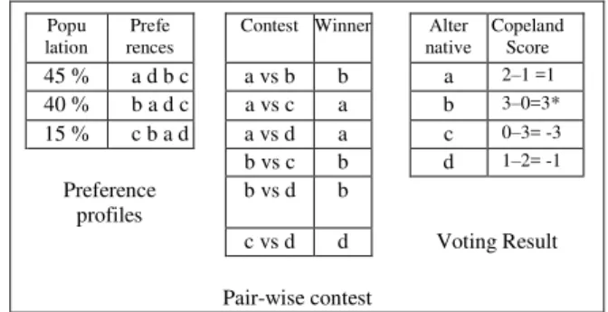
Copeland score is one of the voting methods whose technique is based on a subtraction of the frequency of winning minus the defeat frequency of a pairwise comparison[13]. Another research [14] describes the way the voting method of Copeland Score accommodates decision makers’score based on their respective level of expertise. The example of how to determine pairwise comparisons in the Copeland Score method is presented in Figure 1.

Popu lation

Prefe rences

Contest Winner Alter native

Copeland Score

45 % a d b c a vs b b a 2–1 =1

40 % b a d c a vs c a b 3–0=3*

15 % c b a d a vs d a c 0–3= -3

b vs c b d 1–2= -1

Preference profiles

b vs d b

c vs d d Voting Result

Pair-wise contest

Fig. 1. Determination of pairwise comparisons in the Copeland Score method

Figure 1 above presents three tables, namely the Table of Preference Profiles, the Pairwise Contest Table, and the Table of Voting Results. The Table of Preference Profiles suggests that there are four options, namely A, B, C, and D. 45% of the population prefers A to D, B, and C (see the first row of the Table of Preference Profiles). The Pairwise Contest Table indicates that an option (for exampleA) is compared with all the available options (B, C, D). This pairwise comparison is completedone by one and applies for the overall items of choices.

In the first rowrelating to the pairwise comparison between A and B (see the Table of Preference Profiles), 45% of the population prefers A to B; in the second row, 40% of the population prefers B to A; in the third row, 15% of the population prefers B toA. This implies that there is 45% of the population that prefers A to B, while the remaining 55% (the total number of the population that prefers b) of the population prefers B to A. Thus, B is chosen as the winner of a pairwise comparison between A to B. Comparisons are also made to other candidatesas described above.





;

1

2







_

n

_

j

i ij

i

y

D

;  



 

i i

D D

(5)

The Pairwise Contest Table shows that as the winner, Option Aappears 2x (twice). Option B appears 3x (three times). Option D appears 1x (once), and Option C does not appear.

According to the Pairwise Contest Table, it is revealed that Option A has two chances of winning over C and D, and a chance of losing to B. To determine whether Option A is the best choice or not, a subtraction of the frequency of winning minus the defeat frequency is performed. The Table of the Voting Results shows that Option B has the highest frequency. Based on the frequency, it is decided that Alternative B wins.

III. RESEARCH METHOD

A. Classification of the Types of ICT Projects

The projects in the regional government agencies belonging to ICT projects are [15]:

a)Software Establishment/Development, b)Hardware Provision/Maintenance, c)Network Building/Maintenance, d)Bandwith Purchase/Lease, and

e)Educational Programs/Training for ICT staff

B. The Implemented GDSS Method

Evaluation of ICT projects designedwas a model of

Multiple-Criteria Decision Making (MCDM) using the methods in Multi-Attribute Decision Making (MADM). Determination of the best alternative among a number of alternatives was done based on several predetermined criteria. The scoring criteria to evaluate ICT projects were a compilation of project management concepts in general [16], ISO/IEC 15939 concerning how to measure software [17] and benchmarks that can be used to measure computer performance [18].

Table 2 describes decision makers along with the parameters and criteria used in the evaluation of ICT projects.

TABLE II. CRITERIA OF ICTPROJECT EVALUATION

Output Parameter

Criteria Decision Maker

1 Project Schedule (C1)

Business Process Owner Units (DM1)

2 Project Costs (C2) 3 Project Scope (C3) 4 Project Risks (C4)

ICT Management Work Units (DM2)

5 Project Performance (C5)

Outcome Parameter

Criteria Decision Maker

6 Project Effectiveness (C6)

Executing Parties of Government Institutions (DM3) and

Society represented by DPRD (DM4) 7 Project User Satisfaction

(C7)

Evaluation of ICT projects in government agencies requires assessments undertaken by the Executing Parties of Government Institutions, ICT Management Work Units, Business Process Owner Units, and Society. Stakeholders of the ICT management as a group of decision makers have

specified the assessment criteria based on performance indicators according to the duties and functions. Such performance assessments employed both qualitative and quantitative criteria, where the qualitative criteria used linguistic variables. These linguistic variables referred to variables whose values are indicated in the forms of words or sentences in natural or artificial language [19].

Then, to draw the conclusion relating to the ICT project results attained, the performance assessment scale based on the existing criteria was used. The measurement scale was developed based on the consideration of each decision maker. Table 3 presents the assessment scoring scale used in this research.

TABLE III. ASSESSMENT SCORING FOR CRITERIA PERFORMANCE

Score Assessment Percentage

5 Very

Good Very

Large Ignored 90 s/d 100

4 Fairly

Good

Fairly

Large Minor 80 s/d 89,99

3 Good Large Moderate 60 s/d 79,99

2 Less

Good Less

Large Serious 40 s/d 59,99

1 Not _Good Not _Large Critical < 39,99

C. Scoring for each criteria is elucidated as follows:

 Project Schedule

Based on the criteria of the project schedule timeliness, the percentage between the planned project scheduleand the actual project schedule [20].

Formula:

[1 – ABS (ALT – PLT) / PLT] x 100% (16) ALT=Actual Finish Date – Actual Start Date PLT= Planned Finish Date-Planned Start Date  Project Costs

The ability to provide the agreed scope of duties concerning costs, hours of work, laboratories and travel expenses. Based on the percentage between the committed (baseline) and expected costs (actual + forecast) [20].

Formula:

[1 – (ECost – CCost) / CCost] x 100% (17) Expecteed Cost (Ecost) = actual + forecast Commited Cost (Ccost)

 Project Scope

In this criteria category, the scoring used several linguistic variables, namely: Very Large, Fairly Large, Large, Less Large, and Not Large.

 Project Risks

These refer to the arising impacts of the risks, which are defined as follows [20]:

(6)

ij i

ij

w

r

y



 Serious: If this risk occurs, a project will encounter increases in terms of the costs/ schedule. The minimum requirements of the project that are acceptable can be met while the secondary requirements cannot.

 Moderate: If this risk occurs, a project will encounter increases in terms of the costs/ schedule. The minimum requirements of the project that are acceptable and a few of the secondary requirements can be met.

 Minor: If this risk occurs, a project will encounter slight increases in terms of the costs/ schedule. The minimum requirements of the project that are acceptable and some of the secondary requirements can be met.

 Ignored: If this risk occurs, it will not affect a project. All the requirements can be met.

 Project Performance, Project Effectiveness and Project User Satisfaction

In this criteria category, the scoring used several linguistic variables, namely: Very Good, Fairly Good, Good, Less Good, and Not Good.

Each has its own performance assessment criteria indicated in a measurement scale.

D. The Hybrid Methodof AHP, TOPSIS and Copeland Score

a. Performing criteria scoring(AHP)

b. Calculating normalization values (TOPSIS) c. Calculating weighted normalization values

(AHP-TOPSIS )

(18) Description of the symbols:

- yij refers to weighted normalization values.

- wi refersto the score of each criteria (generated from

AHP scoring)

- rij refers to the normalization value of each

alternativewherei=1,2,...,m; and j = 1,2,...,n

d. Identifying positive and negative ideal solutions (TOPSIS)

e. Calculating the distance between each alternative and the positiveand negative ideal solutions (TOPSIS) f. Determining the proximity value of each alternative

towards the ideal solution (preference) (TOPSIS) g. Repeating steps a to f for each Decision Maker h. Ranking all the DMs (TOPSIS-Copeland Score)

IV. RESULT AND ANALYSIS

This section provides examples of the ICT project evaluation model implementation. The sample data used were retrieved from ten regional government ICT projects that have been completed. In this GDSS model, there were four decision makers (namely DM1, DM2, DM3, and DM4), seven criteria (namely C1, C2, C3, C4, C5, C6, and C7) to assess and ten ICT project alternatives (namely P1, P2, P3, P4, P5, P6, P7, P8, P9, and P10) to evaluate.

DM1 evaluated each alternative based on three criteria C = {C1, C2, C3), DM2 evaluated each alternative based on two criteria C = {C4, C5}, and lastly DM3 and DM4 evaluated each alternative based on two criteria C = {C6, C7}.

a)Performing criteria scoring(AHP)

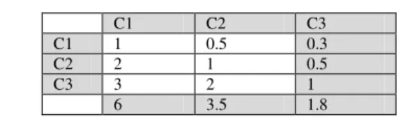
The first step was to create a pairwise comparison matrix of criteria for DM1, followed by scoring the criteria. Then,the total value of aij for each pairwise comparison matrix column

was calculated as shown in Table 4.

TABLE IV. THE PAIRWISE MATRIX FOR THE CRITERIA OF DM1

C1 C2 C3

C1 1 0.5 0.3

C2 2 1 0.5

C3 3 2 1

6 3.5 1.8

After normalization had been completed,the results are presented inTable 5.

TABLE V. SCORES FOR NORMALIZED CRITERIA

C1 C2 C3 Rata-rata

C1 0.1667 0.1429 0.1818 0.1638 W1

C2 0.3333 0.2857 0.2727 0.2973 W2

C3 0.5000 0.5714 0.5455 0.5390 W3

1.0000 1.0000 1.0000 1.0000

b)Calculating normalization values (TOPSIS)

Based on the dataon the evaluation results given by DM1 on the criteria for each ICT project alternative, the following data on assessment results presented in Table 6 are obtained.

TABLE VI. SCORING FOR DM1

C1 C2 C3

P1 4 4 5

P2 3 3 4

P3 5 4 2

P4 4 4 5

P5 3 3 4

P6 5 4 2

P7 4 4 5

P8 3 3 4

P9 5 4 2

P10 4 4 5

12.8841 11.7898 12.6491

TABLE VII. NORMALIZED SCORING FOR DM1(MATRIX R)

R

0.3105 0.3393 0.3953

0.2328 0.2545 0.3162

0.3881 0.3393 0.1581

0.3105 0.3393 0.3953

0.2328 0.2545 0.3162

0.3881 0.3393 0.1581

0.3105 0.3393 0.3953

0.2328 0.2545 0.3162

0.3881 0.3393 0.1581

c)Calculating normalization values (AHP-TOPSIS )

(7)

TABLE VIII. MATRIX (Y) OF DM1

Y

0.0508 0.1009 0.2130

0.0381 0.0756 0.1704

0.0636 0.1009 0.0852

0.0508 0.1009 0.2130

0.0381 0.0756 0.1704

0.0636 0.1009 0.0852

0.0508 0.1009 0.2130

0.0381 0.0756 0.1704

0.0636 0.1009 0.0852

d)Identifying positive and negative ideal solutions (TOPSIS)

A+ 0.0636 0.1009 0.2130

A- 0.0381 0.0756 0.0852

e)Calculating the distance between each alternative and the positive and negative ideal solutions (TOPSIS)

f) Determining the proximity value of each alternative towards the ideal solution (preference) (TOPSIS)

g)Repeating steps a to f for each Decision Maker

After the scoring process had been completed by each DM (DM1, DM2, DM3 and DM4), the following results of project ranking presented in Table 9 were obtained.

TABLE IX. RANKING OF ALL THE DMS

R DM1 DM2 DM3 DM4

1 P1 0.911489 P3 0.614761 P1 0.789999 P1 0.777171

2 P9 0.571017 P10 0.614761 P3 0.707060 P3 0.532960 3 P10 0.553032 P4 0.597624 P4 0.707060 P5 0.532960 4 P8 0.530622 P7 0.597624 P10 0.707060 P10 0.532960

5 P4 0.521865 P2 0.573689 P6 0.675952 P6 0.524957

6 P7 0.521865 P6 0.569533 P9 0.675952 P7 0.524957

7 P5 0.462834 P9 0.569533 P2 0.594851 P9 0.524957

8 P3 0.453630 P8 0.553453 P7 0.594851 P2 0.522668

9 P2 0.435366 P5 0.541074 P8 0.585358 P4 0.522668

10 P6 0.000000 P1 0.453388 P5 0.572409 P8 0.522668

h)Ranking the project evaluation results of all the DMs (TOPSIS-Copeland Score)

The following are the stages ofvoting results for the best ICT projects:

 Preference Profile

The preference profile presented in Table 10 shows that there are a total of ten ICT project alternatives (namely P1, P2, P3, P4, P5, P6, P7, P8, P9, and P10). Each decision maker in the process of decision making had their own score which had been determined according to their respective expertise and competence. The score for DM1 was equal to 0.1, the score for DM2 was equal to 0.4, and the scoresfor DM3 and DM4 were equal to 0.2.

 Performing pairwise contests

A pairwise contest is defined as a paired-comparison process comparing one candidate (alternative) to the other candidates, which was performed by:

- Displaying alternative contests in pairs. For example, P1 is compared with P2, P1 is compared with P3, and so on. Similarly, P2 is compared with P3, P2 is compared with P3, and so on. This pairwise comparisons are taken one at a time and done to all the options until P9 is compared with p10.

- Searching for the winner of the comparisons (contests) of each paired alternative.

- For example, in the contest of the pairwise comparison between P1 and P2 (see Table 11), the winner is P1 as in DM1, P1 ranks 1st while P2 ranks 9th so that the winner in DM1 is P1. In DM2, P1 ranks 10th while P2 ranks 6th, and as a resultP2 wins in DM2. In DM3, P1 ranks 2nd while P2 ranks 7th and consequently the winner in DM3 is P1. Lastly, in DM4,P1 ranks 1st while P2 ranks 8th and thus the winner in DM4 is P1. These imply that the rank of P1 is three times higher than the rank of P2, after calculating the scores of each DM it is revealed that the total score for P1 is equal to 0.1 + 0.3 + 0.2 = 0.6 while for P2 is equal to 0.4. Thus, P1 wins.

TABLE X. PREFERENCE PROFILE

Weight Preferences ( Rangking)

1 2 3 4 5 6 7 8 9 10

DM1

(0.1) P1 P9 P10 P8 P4 P7 P5 P3 P2 P6

DM2

(0.4) P3 P10 P4 P7 P2 P6 P9 P8 P5 P1

DM3

(0.3) P1 P3 P4 P10 P6 P9 P2 P7 P8 P5

DM4

(0.2) P1 P3 P5 P10 P6 P7 P9 P2 P4 P8

TABLE XI. PAIRWISE CONTESTS

Contest Winner

P1

(01+0.3+0.2) VS

P2

(0.4) P1

P1

(01+0.3+0.2) VS

P3

(0.4) P1

P1

(01+0.3+0.2) VS

P4

(0.4) P1

. . .

D+1 0.012712 D-1 0.130907

D+2 0.110520 D-2 0.085217

D+3 0.043126 D-3 0.035806

D+4 0.110088 D-4 0.120157

D+5 0.154066 D-5 0.132746

D+6 0.035516 D-6 0.000000

D+7 0.110088 D-7 0.120157

D+8 0.103272 D-8 0.116746

D+9 0.101414 D-9 0.134992

D+10 0.092180 D-10 0.114053

P1 0.911489 P1 0.911489 Winner

P2 0.435366 P9 0.571017

P3 0.453630 P10 0.553032

P4 0.521865 P8 0.530622

P5 0.462834 P4 0.521865

P6 0.000000 P7 0.521865

P7 0.521865 P5 0.462834

P8 0.530622 P3 0.453630

P9 0.571017 P2 0.435366

(8)

P1

(01+0.3+0.2) VS

P10

(0.4) P1

 Calculating the voting results

The voting results present the results of voting (score) for each candidate afterpairwise contests, based on the following stages:

- Calculating the frequency of winningof the candidates (alternatives) which had been compared using the pairwise contest.

- Calculating the defeat frequency of the candidates (alternatives) which had been compared using the pairwise contest.

- Calculating the differential betweenthe frequency of winningand the defeat frequency of the candidates (alternatives) which had been compared

- Presenting the frequency differential obtained as a score for each candidate.

The voting results are presented in order according to the ranking of the frequency-of-winning scores from the highest to the lowest one for the four DMs, which can be seen in Table 12.

TABLE XII. VOTING RESULTS

Alternatif Win Loss W-L

Proyek 1 9 0 9

Proyek 3 8 1 7

Proyek 10 7 2 5

Proyek 4 6 3 3

Proyek 7 5 4 1

Proyek 6 4 5 -1

Proyek 9 3 6 -3

Proyek 2 2 7 -5

Proyek 8 1 8 -7

Proyek 5 0 9 -9

V. CONCLUSION

This paper offered a hybrid method in MCDM to evaluate ICT projects in Indonesian regional government agencies based on the concept of Group Decision Support Systems (GDSS).

The GDSS concept can overcome any possible inconsistencies which may occur in decision making as it makes decisions based on the mathematical calculation model. Contributionsof the decision makers in the model were in the fom of preferences for choosing ICT Project alternatives based on predetermined criteria using the hybrid method of AHP, TOPSIS and Copeland Score. Based on the implementation examples, projects with the best rank were produced from the assessment undertaken by all DMs, namely Projects 1, 3 and 10 which had the same performance while Project 5 had the worst performance.

Our next research will focus on the development of a web-based prototype to implement the proposed model. The prototype developed attempts to provide an answer to the problems relating to ICT project performance evaluation in regional government agencies.

ACKNOWLEDGMENT

The first author is an employee of Indo Global Mandiri Foundation (Yayasan Indo Global Mandiri, IGM) as a lecturer at Faculty of Computer Science, Indo Global Mandiri University. Now he is pursuing a doctoral program on Computer Science, Department of Computer Science and Electronics, Faculty of Mathematics and Natural Sciences, Gadjah Mada University. This work is supported and founded by IGM.

REFERENCES

[1] T. Bakshi, A. Sinharay, and B. Sarkar, “Exploratory Analysis of Project

Selection through MCDM,” in ICOQM-10, 2011, pp. 128–133. [2] G. Büyüközkan and D. Ruan, “Evaluation of software development

projects using a fuzzy multi-criteria decision approach,” Math. Comput. Simul., vol. 77, no. 5–6, pp. 464–475, May 2008.

[3] S. M. Kazemi, S. M. M. Kazemi, and M. Bahri, “Six Sigma project selections by using a Multi Criteria Decision making approach: a Case

study in Poly Acryl Corp.,” in Proceedings of the 41st International Conference on Computers & Industrial Engineering, 2011, pp. 502–507. [4] H. Ismaili, “Multi-Criteria Decision Support for Strategic Program

Prioritization at Defence Research and Development Canada,”

University of Ottawa, 2013.

[5] M. Ishak, “Kebijkaan Pengukuran Kinerja Pemerintah Daerah,” INOVASI, vol. 6th, pp. 143–151, 2009.

[6] G. J. Victor, A. Panikar, and V. K. Kanhere, “E-government Projects –

Importance of Post Completion Audits,” in International Conference of

e-government (ICEG), 2007, pp. 189–199.

[7] S. Kusumadewi, S. Hartati, A. Hardjoko, and R. Wardoyo, Fuzzy Multi Attribute Decision Making (Fuzzy MADM), First. Jogyakarta: Graha Ilmu, 2006.

[8] H.-J. Zimmermann, Fuzzy Set Theory and Its Applications, Second Edi. Boston, MA: Kluwer Academic Publishers, 1991.

[9] T. L. Saaty, The Analytic Hierarchy Process: Planning, Priority Setting, Resource Allocation. New York, NY: McGraw-Hill, 1980.

[10] T. L. Saaty, Fundamentals of Decision Making and Priority Theory With the Analytic Hierarchy Process. Pittsburgh: RWS Publications, 2000. [11] C.-L. Hwang and K. Yoon, Multiple Attribute Decision Making :

Methods and applications. New York: Springer Berlin Heidelberg, 1981. [12] S. K. Cheng, “Development of a Fuzzy Multi-Criteria Decision Support System for Municipal Solid Waste Management .’ A Thesis,” University of Regina, 2000.

[13] B. Gavish and J. H. Gerdes, “Voting mechanisms and their implications

in a GDSS environment,” Ann. Oper. Res., vol. 71, pp. 41 – 74, 1997. [14] Ermatita, S. Hartati, R. Wardoyo, and A. Harjoko, “Development of

Copeland Score Methods for Determine Group Decisions,” Int. J. Adv. Comput. Sci. Appl., vol. 4, no. 6, pp. 240–242, 2013.

[15] H. Setiawan, J. E. Istiyanto, R. Wardoyo, and P. Santoso, “The Use of KPI In Group Decision Support Model of ICT Projects Performance Evaluation,” in International Conference on Electrical Engineering, Computer Science and Informatics (EECSI 2015), 2015, no. August, pp. 19–20.

[16] PMI, A Guide to the Project Management Body of Knowledge - PMBOK Guide. 2013.

[17] ISO/IEC, Information technology — Software engineering — Software measurement process, no. September. 2001.

[18] “Standard Performance Evaluation Corporation.” [Online]. Available: https://www.spec.org/. [Accessed: 02-Jan-2016].

[19] L. A. Zadeh, “The Concept of Linguistic Variable and ITs Application to Aprroximate Reasoning-II,” in Information Sciences, vol. 357, 1975, pp. 301–357.