Sundarapandian et al. (Eds): ICAITA, SAI, SEAS, CDKP, CMCA, CS & IT 08,
pp. 231–243, 2012. © CS & IT-CSCP 2012 DOI : 10.5121/csit.2012.2520
Quan Yuan
1and Ji Yeong Lee
and Changsoo Han
1
Department of Mechanical Engineering, Hanyang University, Ansan, Korea [email protected]
ABSTRACT
This paper presents an algorithm, based on conventional GVG that enables a car-like robot find a collision free path from depart configuration to some goal position in an environment containing some convex obstacles. Prior research on GVG prescribed path for a circular robot. The circular robot is holonomic system, but this time GVG is used in nonholonomic system. The proposed algorithm enables the car-like robot depart the GVG to the goal position with the nonholonomic path.
K
EYWORDSsensor based, nonholonomic, departability, GVG roadmap, convex set.
1.
I
NTRODUCTIONThe motion planning problem is a well-known problem in the field of robotics. In this paper we deal with car-like robots which move in a planar environ-ment. Our objective is to find a collision free path in an unknown closed environment containing some convex obstacles for a car-like robot from a depart confi-guration to a goal position. The algorithm should be sensor based.
A. History and Related Work
In the past years, techniques of motion planning for holonomic system robotics were developed. Holonomic motion planning techniques has been already mature. The main techniques can be divided into three classes: roadmap methods, cell decomposition methods, and potential field methods. T.Lozano-perez developed the Visibility Graph algorithm, which is used for mobile robot to find Euclidean shortest paths among a set of polygonal obstacles in the plane [5]. H.Choset defined Generalized Voronoi Graph, which is a roadmap of the environment; using this road map, the mobile robot can reach any point in the environment [6]. Holonomic system robotics can follow the roadmap precisely, however, the algorithm cannot be implemented in the nonholonomic system directly. Research area of nonholonomic robots’ navigation is also vast. Many algorithms were developed for like robots. Huifang Wang defined an algorithm for car-like robots to find a shortest path between two configurations without obstacles [7]. There’s another optimal algorithm for car-like robots is proposed in [8], Vendittelli gave a method to calculate the nonholonomic distance from a configuration to a position.
algorithms is called “Bug algorithm” proposed by Lumelsky [2].This algorithm is mathe-matically complete. The other approach is an incre-mental procedure to construct GVG [1,3], It requires only line of sight information. This algorithm has been successfully implemented on an actual mobile robot with a ring of sonar sensors [9]. Unfortunately, the algorithm cannot be applied to car-like mobile robot because GVG is not smooth. To solve the problem, K. Nagatani proposed a method in [10] to deform the GVG to be smoothly to enable car-like robots’ following by maximizing an evaluation function. In this algorithm, the local GVG and C-space are constructed by conventional algorithm. They just focused on the evaluation function and how to generate candidates of smooth path.
In conventional GVG, the departability is a simple step for point robot, but it is big challenge for car-like robot. The method is solved in this paper.
In previous work, we develop the algorithm for car-like robot to access and trace the GVG in [11]. We can also generate the completed GVG. In this paper, we develop the follow-on work: generating a nonholonomic path from the depart configuration to the goal point.
B. Contribution
This paper proposed a sensor-based approach for car-like mobile robot to depart the GVG. The GVG is a 1-dimensional network of curves, which can be used as a basis for a roadmap or “retract-like” structure. Roadmaps or retract retract-like structures capture the global topological properties of the robot’s free space and have the following important properties: accessibility, departability and connectivity [4]. The GVG structure has advantages for expressing the paths of mobile robots for sensor-based navigation from the point of view of ‘safety’ and ‘completeness’. However, it has the limitation for nonholonomic system. When the point robot depart the GVG, it can generate a straight collision-free path from depart configuration to the goal position. However, the nonholonomic robot cannot follow the straight path, and it may collide with obstacles. We need to find a method to generate a collision-free nonholonomic path for car-like robot to reach the goal.
Our outline of this paper is as follows: Section 2 is the most important part of the paper; this part presents the departability path. Section 3 presents some simulation results and in Section 4 we discussed the future direction.
2.
K
INEMATICM
ODELO
FT
HER
OBOTThe configuration of a car-like robot, sketched in Fig.1, at the instant t is completely defined in
C=R2×S1expressed byq=
(
p,θ
)
T =[ ( ), ( ), ( )]x t y tθ
t T, p∈R2by the position p=(x t( ),y t( ))T of the reference point and the heading directionθ
( )
t
of the robot. The model of the car-like robot which we will refer in this paper is described by the following control system.cos ( ) 0
sin ( ) 0
0 1
t
q t v
θ
θ
ω
= +
& (1)
sin ( ) cos ( ) 0
x&
θ
t −y&θ
t = (2)Equation (2) represents a velocity constraint where the velocity of the center of the mobile robot’s wheel does not have any lateral components. Here we assume the mobile robot is reasonably slow such that the longitudinal traction and lateral force exerted on the tires do not exceed the maximum static friction between the tires and the floor. It’s called no-slip condition.
At the low speed of the car-like robot, the kinematic steering is determined from the Ackerman turning geometry as =b/R=b where is the equivalent steering angle for the front wheels, b is the wheelbase, and R is the turning radius. And due to the maximum value of the equivalent steering angle for the front wheels max, the lower limit on the turning radius is given by Rmin.
As shown in the picture, GX-GY is the global coordinate system which is fixed. RX-RY is the robot coordinate system which is a moving coordinates attached to the robot.
In this paper we use the path symbol such as:Cl+,Sl−. Cl+is a curve with l length, and “+” means the velocity is positive. C can be L or R, which means turn left or right with minimum turning radius. Sl−
is a straight segment with l length, and “-” means the velocity is negative.
Fig.1 Kinematic model of the mobile robot
3.
I
NTRODUCTIONO
FC
ONVENTINALGVG
Definition (Distance function): Single Object Distance Function. The distance between a car-like
robot configuration q= (p, ) T and a convex set QOiis
( ) min i i c QO
d q p c
∈
= −
(3)
where ||·|| is the 2-norm in Rm. In [8] it is shown that the gradient of di(q) is
0
0
( ) i
p c d q
p c − ∇ =
−
QOi. For convex sets, the closest point is always unique. di(q) and ∇d qi( ) can be computed from sensor data.
The basic building block of the GVG is the set of points equidistant to two sets QOi and QOj, which can be defined as the following equation
0 ) ]( [
)
(q = d −d q =
G i j (5)
A meet point is a point where the GVG edges meet. A meet point is (at least) triple equidistance to the closest obstacles and is defined as
. 0 ) ( )
( =
− −
= q
d d
d d q G
k i
j i
(6)
In 2-D space, GVG is connected.
The concept of the navigation proposed in this paper is based on GVG, and combine the nonholonomic departability path to reach the goal. We consider a car-like mobile robot operating in a bounded subset Q of a 2-dimensional Euclidean space. Q is populated by obstacles QO1…, and
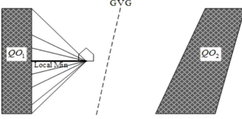
QOn which are the convex sets. It is assumed that the boundary of Q is a collection of convex sets, which are members of the obstacle set {QOi}. In this paper, we assume the car-like robot is equipped with range sensor and the range sensor is an infinite laser scanner, and the field of view is infinite too. As shown in the Fig. 2, the thick ray, labeled local minimum, corresponds to the smallest sensor reading. The robot will move in the direction indicated by the black arrow to access the GVG, denoted by a dashed line between two nonparallel walls.
Fig. 2 The unlimited sensor
4.
D
EPARTABILITYP
ATHDepartability is the property where a robot can find a collision free path from the GVG to the goal. For holonomic robot the robot can access the goal in a straight line. However, that method is not suitable for nonholonomic robot because of the turning radius limitation. Therefore, a new method is needed for car-like robot departing from GVG to the goal. In this method, we define the depart configuration as the configuration to leave the GVG, and the path from the depart configuration to the goal is the depart path.
the boundary of the Voronoi Region is a subset of GVG. In other words, if QO is a set of n
distinct obstacles in space,and the point p lies in a region containing QOi then
i
j
QO
QO
QO
p
d
QO
p
d
(
,
i)
<
(
,
j)
,
i∈
,
≠
(7)
If the goalpgoalis in the Voronoi Region of QOi, then the depart point should be on the boundary of the Voronoi Region to make the robot trace the roadmap as much as possible. The depart point is defined as below:
Definition (depart configuration): firstly, the coordinates of the depart configuration is on GVG. Secondly, the goal point pass through the segment that connects the depart coordinates and the closest point of the obstacle. The function is as follows:
{
q p R S p GVG c p c p p p}
qd = ( , )∈ × , ∈ | m− = m− goal + goal − 1
2
θ
(8)
where cm is the closest point of obstacle and p ∈R 2
is the position of the car-like robot. The coordinates of the depart configuration are unique, but the direction is not.
1
c c2
d
q
goal
p 1
QO
Fig. 3 Depart configuration in GVG
Uniqueness proof of depart configuration:
GVG
1
d
q
2d
q
1
c
2
c
1
l
2
l
Claim: there is a unique depart configuration in the voronoi region for the closest obstacle.
Proof: if the depart configuration is not unique, as shown in the figure, qd1 and qd2 are the two depart configurations, as shown in Fig. 11.
qd1 and qd2 are the depart configurations; c1 and c2are the closest point respectively.
c1 is the closest point, and then we can get the tangent line of c1, denoted as T1
∵c1∈QOi,l1 is the tangent line pass through c1 , and the obstacle QOiis convex
∴QOi⊆Ⅰ Ⅲ,QOi Ⅱ=ø
∵c2∈ QOi,l2 is the tangent line pass through c2.
∴QOi⊆Ⅱ Ⅲ,QOi Ⅰ=ø
∵c2∈Ⅱ,
c
1∈
Ⅰ∴it is contradicting with the previous conditions.
∴we can get the conclusion that the depart configuration is unique.
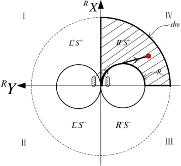
After obtaining the coordinates of the depart configuration, the path from the depart configuration to the goal is generated. As shown in Fig. 3, qd is the depart configuration; dm is the minimum distance; Rm is the minimum turning radius of a car-like mobile robot. Because dm is the minimum distance to the obstacles in the environment, so we can get a collision free space which is a circle with qd as the center and dm as the radius. We can obtain different nonholonomic paths to the goal under different conditions:
(1) Region C|S : If the goal is outside of the minimum turning radius circles and dm >0, then with different position of the goal, there are 4 types of nonholonomic paths. Details are shown in Fig. 5, if the goal is located in the shaded area in the fourth quartile, the nonholonomic path to reach the goal is R+S+. If the goal is located at the symmetrical area in the other three quartiles, the nonholonomic path is also symmetrical with that of the fourth quartile. The paths are displayed in Table1 where v is the length of the arc and l is the length of the path. Then we can calculate v and l from the equations shown below:
−
−
−
=
−
+
=
min min min min min min min)
sin(
)
(
)
cos(
)
cos(
)
(
)
sin(
R
R
v
v
l
R
v
R
y
R
v
v
l
R
v
R
x
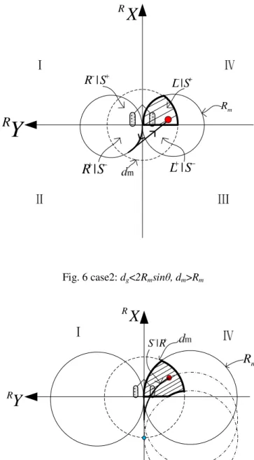
g g (9) (2) Region C|S: If the goal is inside of the minimum turning radius circlesand dm >Rm , then with+
−
−
−
=
−
−
=
min min min min min min min)
cos(
)
sin(
)
(
)
sin(
)
cos(
)
(
R
R
v
R
R
v
v
l
y
R
v
R
R
v
v
l
x
g g (10) (3) Region S|C: If the goal is inside of the minimum turning radius circlesand dm <Rm, the robotcannot calculate a direct path to the goal. At this time, the robot can go straight forward or backward. As shown in Fig. 7, we know that the goal is located in the fourth quartile. We can calculate the path
S
l u−|
C
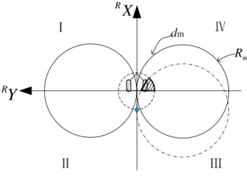
u+− by Eq. 11, if l-u is smaller than dm, the robot will follow this path. When l-u is larger than dm, if the robot followed the path, it will exit to a safe space. Here u is the length of the curve and l is the length of the path. Then we can calculate u and l from the equations below: − − = + − = min min min min min ) cos( ) cos( 2 ) sin( ) sin( 2 R R l R u y R l R u x g g (11) (4) Region S|C…C|S or S|C…CS: In this region, the robot cannot reach the goal to follow the
paths above. As shown in Fig. 8, when the robot arrives at the boundary of the free space, the goal is detected not to have been directly arrived. In this case, the robot follows R+ until it arrives at the boundary again, then follows L-, if the direction of the robot is not towards the goal, then it follows the C segment until the robot can reach the goal. The departability paths are summarized as S|C…C|S or S|C…CS.
+ + S R + + S L − −
S
L
R
−S
−X
RY
R
m R|
L S
− +|
R S
− +|
R S
+ −L S
+|
−X
R
Y
R
m
R
Fig. 6 case2:dg<2Rmsin , dm>Rm
X
R
Y
Rm
R
|S R− +
X
R
Y
Rm
R
Fig. 8 case4: dg<2Rmsin , 0<dm<Rm
To aid understanding, the paths are displaced in Table 2. With different goal points,
we achieve different paths.
Table1 Departability of the different paths
dg dm quadrant path
dg>2Rmsin
(the goal is outside of the minimum turning radius circles)
dm>0
Ⅰ L+S+
Ⅰ L-S
-Ⅰ R-S
-Ⅰ R+S+
dg<2Rmsin
(the goal is inside of the minimum turning radius)
dm>Rm
Ⅰ R-|S+
Ⅰ R+|S
-Ⅰ L+|S
-Ⅰ L-|S+
0<dm<Rm
Ⅰ S-|L+or S|C…CS
Ⅰ S+|L- or S|C…CS Ⅰ S+|R- or S|C…CS Ⅰ S-|R+or S|C…CS
5.
S
IMULATIONR
ESULTSshowed that the robot can reach the goal follow the C|S path to reach the goal. The third picture shows that the robot can reach the goal follow S|C path to reach the goal. The forth one shows that the robot can reach the goal by the S|C…C|S or S|C…CSmotion. From the results, we can see that the robot can reach the goal in the four cases.
0 2 4 6 8 10 12
0 5 10 15
Fig. 9 GVG generation
-3 -2 -1 0 1 2 3
-3 -2 -1 0 1 2 3
-2.5 -2 -1.5 -1 -0.5 0 0.5 1 1.5 2 2.5 -2.5
-2 -1.5 -1 -0.5 0 0.5 1 1.5 2 2.5
dg<2Rmsin , dm>Rm
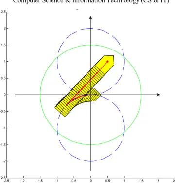
Fig. 11Case3: S|C Goal(0.25,044),dm=0.6,Rmin=1
-2.5 -2 -1.5 -1 -0.5 0 0.5 1 1.5 2 2.5
-2.5 -2 -1.5 -1 -0.5 0 0.5 1 1.5 2 2.5
-2.5 -2 -1.5 -1 -0.5 0 0.5 1 1.5 2 2.5 -2.5
-2 -1.5 -1 -0.5 0 0.5 1 1.5 2 2.5
S|C...C|S
path free space boundary Rmin circles target
Fig.13 Case4: S|C…C|S Goal(0.1,0.5) dm=0.6,Rmin=1
Based on the accessibility, traceability and departability, we are given an initial configuration and a goal position in the unknown environment to find a collision free path between them.
-2 0 2 4 6 8 10 12
-2 0 2 4 6 8 10 12 14
6.
CONCLUSIONThis algorithm enables the car-like mobile robot find the depart configuration and generate a path to leave the GVG to the goal. Then a nonholonomic path from the initial configuration to the goal point in unknown environment is generated incrementally. Combined with the conventional GVG, the path is generated with equidistance condition, which makes the car-like robot avoid the obstacles.
A
CKNOWLEDGEMENTS“This research was supported by the MKE(The Ministry of Knowledge Economy), Korea, under the ‘Advanced Robot Manipulation Research Center’ support program supervised by the NIPA(National IT Industry Promotion Agency)”(NIPA-2012-H1502-12-1002)
R
EFERENCES[1] H.Choset and J.Burdick,” sensor-based motion Planning II: Incremental Construction of Generalized Voronoi Graph”, Conference: International Conference on Robotics and Automation-ICRA,vol.2,pp.1643-1648 vol.2,1995
[2] V.Lumelsky and A.Stepanov.Path Planning Strategies for point Mobile Automation Moving Amidst Unhknown Obstacles of Arbitrary Shape. Algorithmica, 2:403-430, 1987.
[3] H.choset, I. Konukseven, and J. Burdick, “mobile robot navigation: Issues in implementation the generalized voronoi graph in the plane” in Proc.of IEEE/MFI, (Washington DC), 1996.
[4] H.Choset and J.Burdick,’’sensor-based Planning I: Generalized Voronoi Graph”, in Proceedings of the 1995 IEEE International Conference on Robotics and Automation(ICRA’95),pp. 1649-1655, May,1995
[5] T. Lozano-Perez and M. Wesley. An algorithm for planning collisionfree paths among polyhedral obstacles. Communications of the ACM, 22(10):560–570, 1979.
[6] H. Choset and J. Burdick. Sensor based motion planning: Incremental construction of the hierarchical generalized Voronoi graph. International Journal of Robotics Research, 19(2):126–148, February 2000.
[7] Huifang Wang and Yangzhou Chen and Soueres,P, “An efficient geometric algorithm to compute time-optimal trajectories for a car-like robot”, 2007 46th IEEE Conference on Decision and Control, Publisher, New Orleans, LA, 12-14 Dec. 2007, pp. 5383-5388.
[8] M.Vendittelli, J.laumond, and C.Nissoux, “Obstacles distance for car-like robots,” IEEE Trans. on Robotics and Automation,15(4),1999.
[9] K.nagatani, H.Choset, and S.Thrun, “Towards exact location without explicit localization,” Proc.of IEEE International Conf.on Robotics and Automation, PP. 342-348,1998.
[10] K. Nagatani, Y.Iwai and Y.Tanaka, “Sensor based navigation for car-like mobile robots using Generalized Voronoi Graph,” Proc. of IEEE/RSJ International Conf. on Intelligent Robots and System, PP. 1017-1022. 2001
[11] Q.YUAN, Ji Yeong Lee and Changsoo Han, “Sensor-based Navigation Algorithm for Car-like Robot to Generate the Completed GVG ,” 2011 11th International Conference on Control, Automation and Systems (ICCAS), PP1142-1147. 2011
Author QUAN YUAN