Car Like Mobile Robot calibration to
reduce Effects of Systematic Errors.
Mr.Chittaranjan Mahajan Dr. S. D. Lokhande
Sinhgad College Of Engineering, Sinhgad College Of Engineering,
Pune,India Pune,India.
Abstract: This paper is focused on systematic errors on car like mobile robot (CLMR).Dead reckoningis a mathematical procedure for determining the present location of a object by advancing some previous position through known course and velocity information over a given length of time. If systematic error is present in CLMR then it is difficult to localize the position of CLMR. This paper proposes method to find out the systematic errors that are present in CLMR and reduce them.
Key Words: Dead reckoning , CLMR, Systematic error, Odometry.
I. ERRORS IN ODOMETRY
Odometry is based on simple equations that are easily implemented and that utilize data from inexpensive incremental wheel encoders. However, Odometry is also based on the assumption that wheel revolutions can be translated into linear displacement relative to the floor. This assumption is only of limited validity. One considerable example is wheel slippage: if one wheel was to slip on, because of an oil spill, then the associated encoder would read wheel revolutions even though these revolutions would not correspond to a linear displacement of the wheel. Along with the extreme case of total slippage, there are several other factors are also plays an important role for inaccuracies in the translation of wheel encoder readings into linear motion. All of these error sources fit into one of two categories: systematic errors and non-systematic errors [4].
1.Systematic Errors
Systematic errors are vehicle specific and don’t usually change during a run (although different load distributions can change some systematic errors quantitatively). Thus, Odometry can be improved generally (and in our experience, significantly) by measuring the individual contribution of the most dominant errors sources and then counteracting their effect in software. Among all unequal wheel diameters and uncertainty about the wheelbase are most dominant errors causing systematic errors. The following are some example of it.
1. Unequal wheel diameters.
2. Average of actual wheel diameters differs from nominal wheel diameter. 3. Actual wheelbase differs from nominal wheelbase.
4. Misalignment of wheels. 5. Finite encoder resolution. 6. Finite encoder sampling rate. 2.Non-Systematic Errors
Nonsystematic Odometry errors are those errors that are caused by interaction of the robot with unpredictable features of the environment. For example, irregularities of the floor surface, such as bumps, cracks, or debris, will cause a wheel to rotate more than redirected, because the affected wheel travels up or down the irregularity, in addition to the expected horizontal amount of travel. Nonsystematic errors are a great problem for actual applications because it is impossible to predict an upper bound for the Odometry error. The following are some example of it.
1. Travel over uneven floors.
2. Travel over unexpected objects on the floor. Wheel-slippage due to:
1. Slippery floors. 2. Over acceleration. 3. Fast turning (skidding).
4. External forces (interaction with external bodies). 5. Internal forces (castor wheels).
6. Non-point wheel contact with the floor.
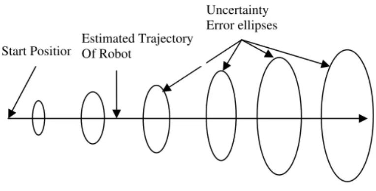
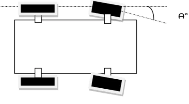
Figure 1: Error ellipses.
It is noteworthy that many researchers develop algorithms that estimate the position uncertainty of a dead-reckoning robot .With this approach each computed robot position is surrounded by a characteristic “error ellipse” ,which indicates a region of uncertainty for the robot's actual position [1].Typically, these ellipses grow with travel distance, until an absolute position measurement reduces the growing uncertainty and thereby “resets” the size of the error ellipse. These error estimation techniques must rely on error estimation parameters derived from observations of the vehicle's dead-reckoning performance. Clearly, these parameters can take into account only systematic errors, because the magnitude of non-systematic errors is unpredictable.
II. ROBOT MECHANISM
A car like mobile robot (CLMR) developed for the experimentation is shown in figure 2. It has four wheels which are made from wood and rubber is coated on wheel so that it will maintain proper grip on floor . The mechanism of CLMR is shown in Figure 3.
Out of four wheels, rear two wheels are coupled on the same axel which are used to provide a linear motion; Front two wheels are capable of doing the steering action to control the displacement of the robot. The mechanism made in a such a way that it will be easy to add the errors for study purpose.
Figure 2 : Car like Mobile Robot (CLMR).
There are to encoders are used one is incremental and another is absolute encoder. Incremental encoder is attached to the common axel of rear wheel to count a pulses when robot moves.
Start Position Estimated Trajectory Of Robot
M= DC motor.
AE = Absolute Encoder. IE = Incrementing Encoder.
Figure 3 : CLMR construction
The pulses are reflects the distance travelled by the robot. The absolute encoder is attached to the steering wheel so that we will get the angle through which the robot is turning.
III. BLOCK DIAGRAM OF ELECTRONIC HARDWARE
Figure 4: Block diagram of electronic hardware..
A main electronics board holds a 89V51RD2BN micro-controller. Microcontroller operates the traction and steering motors through an L298D DC motor controller IC, simultaneously it records the incoming pulses from the incremental encoder as well as absolute encoder and making all required dead reckoning calculations. An LCD is connected to display real time information about the current angle and position of the robot. Opto-isolators are used for isolation. The keyboard is used to enter the co ordinates as well as the calibration parameters. The EEPROM is used to hold the calibration parameters. The Pulse Width Modulation technique is used to control the speed of the DC motors.
IV.ODOMETRY EQUATIONS
Microcontroller Opto
Isolator 8 I/P
Opto Isolator
2 I/P
EEPROM
LCD Display
DC Motor
Driver
Key Board
r
M+AE
moving along the curve are studied separately.
Calibration parameters are calculated separately which will be considered at the time of respective movement.
Distance Travelled D = Kd x δe ---(1)
= Calibration parameter x encoder count
= r x Δφ ---(2)
= Radius of wheel x angle of rotation of wheel.
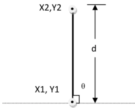
To consider the effects of the systematic error on the CLMR when it is moving along straight from location (X1,Y1) to next location (X2,Y2) with angle θ = 90º.
Figure 5 :CLMR movement along straight Line.
If there is no error then it will move along the line shown in fig . 5.The next position of the CLMR can be given as below,
X2 = X1 ---(3)
Y2 = Y1 + d ---(4)
where d = distance to be travelled by Robot
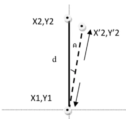
If there is any error then it will move along straight line but with certain angle with predefined path. In this condition, next position of the CLMR can be given as below,
X2 = X1 + d * cosθ ---(5)
Y2 = Y1 + d * sinθ ---(6)
Where θ is angle of inclination.
Case 1: If inclination towards right see fig. 6.
X1, Y1 X2,Y2
Figure 6 : CLMR movement along straight Line with angle(90- θ)
Then we will get following odometry equations for new X2,Y2 which is represented as X’2,Y’2 as follows:
X’2 = X1 + d * sin( θ) ---(7)
Y’2 = d * cos ( θ)--- ---(8)
From above equation we can a choose proper value of θ to reduce the error. Here this θ is the calibration factor which is added/subtracted every time whenever CLMR is supposed to be traversing in straight line .
Case 2: If inclination towardsLeft see figure 6
Figure 7 : CLMR movement along straight Line with angle(90+ θ).
Then we will get following Odometry equations for new X2, Y2 which is represented as X’2,Y’2 as follows:
X’2 = X1 + d * cos (90 + θ) ---(9)
Y’2 = Y1 + d * sin (90 - θ) ---(10)
From above equation we can a choose proper value of θ to reduce the error. Here this θ is the calibration factor which is added/subtracted every time whenever CLMR is supposed to be traversing in straight line .
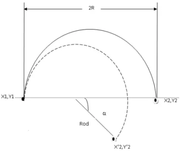
Case 1: If inward the curvature path, see fig. 8
X1,Y1
X2,Y2 X’2,Y’2
θ
d X1,Y1
X’2,Y’2 X2,Y2
Figure 8: CLMR movement along curvature path with less Steering radius Rod
The distance travelled by the robot from point X1,Y1 to X’2,Y’2 is same as distance to be travelled from point X1,Y1 to X2,Y2 . But with less radius Rod. The length of the curvilinear paths S is same for original and new path
S= R x π
S = Rod x (π + α)
R x π = Rod x (π + α)
Rod =R x π/ (π + α) ---(14)
Therefore, the next position of the CLMR will be as follows,
X’2 = Rod + Rod * cos( α )---(15)
Y’2 = Rod *sin (α )---(16)
Case 2: If outward the curvature path, see fig. 9
Figure 9: CLMR movement along curvature path with more Steering radius Rod
S= R x π
S = Rod x (π - α)
R x π = Rod x (π - α)
Rod =R x π/ (π - α) ---(18)
Therefore, the next position of the CLMR will be as follows,
X’2 = Rod + Rod * cos( α )---(20)
Y’2 = Rod *sin (α )---(21)
V.TESTING AND RESULTS
For testing and calibration we have written a software in a such a way that the robot can operate in two mode the calibration mode as well as a normal mode. To differentiate this mode a routine is assigned which will check the status of the CAL key as soon as the microcontroller come out from the RESET condition. If this key is pressed then it will enter in calibration mode. Now we can take different test and enter the calibration parameters. Then we RESET the processor again now the CAL key is impressed so robot will work in normal mode . Now we can enter the path or co-ordinates and we can check the effect of the systematic error.
To support our method of calibration ,we have carried out some experiments.
Case 1 : Calibration of error because of wheelbase
After introducing the error in wheelbase as shown in fig 10, the robot moved on preprogrammed paths that is along a straight line as shown in fig 11 as well as on curvature path as shown in fig 12 .
Figure 10: Error in wheel base in wheel base
For testing traversal along straight line.
the distance between (X1,Y1) and (X2,Y2) is kept as 250 cm and angle θ = 90 . After a introducing error, it is again moved along straight line .But because of error robot moves with certain angle i.e. (90 – θ ) with the proposed path from (X1,Y1) to (X’2,Y’2). Equations 7 and 8 are used to make the calibration. After calibration the angle of diversion reduced (see fig. 11).
Figure 11: Testing and calibration of the CLMR movement along the straight line. For testing traversal along curvature
The distance between (X1,Y1) and (X2,Y2) is kept as 1000cm and steering angle 20 degree . After a introducing error, it is again moved along curvature .But because of error introduced their will be change in the steering radius. Equation 20 and 21 are used to make the calibration. After calibration the error because of steering radius is reduced (see fig. 12) .
Figure 12: Testing and calibration of the CLMR movement along the curvature path.. Case 2 : Calibration of error because of change in radius of wheel.
Figure 13: Change in radius of wheel
For testing traversal along straight line
The distance between (X1,Y1) and (X2,Y2) is kept as 250 cm and angle θ = 90 . After a introducing error, it is again moved along straight line .But because of error robot moves with certain angle i.e. (90 – θ ) with the proposed path from (X1,Y1) to (X’2,Y’2). Equations 7 and 8 are used to make the calibration. After calibration the angle of diversion reduced (see fig. 14).
Figure 14: Testing and calibration of the CLMR movement along the straight line.
For testing traversal along curvature
The distance between (X1,Y1) and (X2,Y2) is kept as 1000cm and steering angle 20 degree . After a introducing error, it is again moved along curvature .But because of error introduced their will be change in the steering radius. Equation 20 and 21 are used to make the calibration. After calibration the error because of steering radius is reduced (see fig. 15) .
r
Figure 15: Testing and calibration of the CLMR movement along the curvature path..
VI. CONCLUSION
Systematic errors are major source of errors in dead reckoning, it affect the localization of robot .To improve the accuracy in car like mobile robot localization, it is needed to calibrate a robot frequently. To calibrate the robot the cumulative effect of the systematic errors are considered so it will require less calculation to find out the calibration parameter. The method for calibration proposed in this paper is easy, require less calculations.
REFERENCES
[1] Kooktae Lee and Woojin Chungr, “Calibration of kinematic parameters of a Car like Mobile Robot to improve Odometry Accuracy”, International Conference on Robotics and automation At Pasadena, CA, USA, may 19-23,2008.
[2] Kooktae Lee , Woojin Chung' , Hyo Whan Chang' , Pal Joo Yoon, “Odometry Calibration of a Car-Like Mobile Robot”, International Conference on Control, Automation and Systems 2007Oct. 17-20, 2007 in COEX, Seoul, Korea.
[3] Philips J,M Kerrow,Danny Ratner, “Calibrating a 4-wheel mobile robot”, International Conference on intelligent Robot and systems,EPFL,OCTOBER 2002.
[4] Johann Borenstein, Member, IEEE, and Liqiang Feng, “Measurement and Correction of Systematic Odometry Errors in Mobile Robots”,IEEE TRANSACTIONS ON ROBOTICS AND AUTOMATION, VOL. 12, NO. 6, DECEMBER 1996.
[5] Yang Cheng, Mark W. Maimone and Larry Matthies, “Visual Odometry on the Mars Exploration Rovers”, IEEE Robotics & Automation Magazine 1070-9932/06/$20.00©2006 IEEE.
[6] Youngblut C, Johnson RE, Nash SH, Wienclaw RA, Will CA., “Review of Virtual Environment Interface Technology”, Internal report P-3186, Institute for Defense Analyses (IDA), Alexandria, VA, 1996, Available
[7] Borenstein J, Everett HR, Feng L., “Where am I? Sensors and Methods for Mobile Robot Positioning”, Technical Report, University of Michigan, 1996, Available Internet: