The Determinants of Actual Migration and the Role of Wages and Unemployment in Albania: an Empirical Analysis

The Determinants of Actual Migration and the Role

of Wages and Unemployment in Albania: an

Empirical Analysis

Cristina Cattaneo

Fondazione Eni Enrico Mattei, University of Sussex and Università Carlo Cattaneo - LIUC

Abstract

The paper explores the determinants of internal migration in Albania, adopting the Harris-Todaro approach to migration: an internal migration function is estimated using district wage and unemployment rate differentials. The aggregate level wages and unemployment, included in the migration equation, are retrieved from a first stage wage and unemployment equations, estimated controlling for personal characteristics. Moreover, in order to test the predictions of the human capital model of migration, the difference between migrants and non-migrants is emphasized in the estimation. The data source is the “Living Standard Measurement Survey for Albania” (2002), undertaken by the national Institute of Statistics and the World Bank jointly. The results reveal that both wage and unemployment differentials are important determinants of the propensity to migrate in Albania. This conclusion is further emphasized by noting that migrants gain substantially in terms of higher returns to individual characteristics after emigration.

JEL Classification: J61, J31, J64, P2

Keywords: Internal Migration, Wage, Unemployment, Transitional Economy

1. Introduction

Albania is one of the economically least developed countries in Europe: after the collapse of the communist regime a substantial growth was achieved but poverty at the household level is still very high. A strong link exists between poverty and unemployment, i.e., the lack of employment is one of the main determinants of poverty: it is reported that more than half of the families with an unemployed household head are poor and the situation is particularly difficult in the rural districts. The registered unemployment rate was 14.5 percent for the 2001, which rises to 15.3 percent, when the standard definition of unemployed is extended to seasonal workers and discouraged workers (World Bank, 2003).

The high rates of unemployment and the severe poverty experienced by the household may have induced strong pressure toward migration. Albanians are the most inclined to leave their country among all citizens of transition countries. According to a study conducted by the International Organization for Migration (Stacher and Dobernig, 1997), in 1993 over half of Albanians were willing to move and more striking, a fifth of them permanently. Statistics are poor, partly due to the irregular nature of much of migration, but most rough estimates of migration suggest that at least 15% of the population lives abroad and 40 percent of the people have some relatives settled outside the borders of the country (UN, 2002). External migration is not the only pattern in Albania, as there is a high rate of internal migration as well. The most

∗

common form of internal migration is urbanization: the urban population has risen from 31.8% in 1970 to 42.0% in 2000 (UN, 2002); however, migration occurs also from the internal areas toward the coastal regions and from the north to the south, because economic conditions are less severe in the southern than in northern areas.

The lack of relevant household data, however, has constrained any attempt to analyse the process governing migration behaviour in Albania and its determinants. In fact, no structured household surveys were available prior the LSMS 2002, which is the data source for this research: this limitation prevented any worthwhile analysis of the Albanian experience. This research aims to fill the current gap in knowledge, providing a detailed analysis of wage and unemployment equations at individual micro level as well as examining the internal migration pattern.

The ultimate objective of the paper is two-fold. On the one hand it analyses internal migration at an aggregate district level, adopting the Harris-Todaro approach: an internal migration function is estimated using aggregate wage and unemployment rate differentials. The distinct feature of this work is that the district level variables are endogenously calculated from a first stage wage and employment equations: this is done to control for individual heterogeneity, in accordance with the human capital model in migration. The second objective is to emphasize the different performance of migrants and non-migrants in the individual-level wage and unemployment equations: interpreting the coefficients of the movers and non-movers variables, in fact, the existence of economic gains from migration are highlighted.

The remainder of the paper is organized as follows. Section 2 presents the existing studies. Section 3 details the data set used and provides a preliminary description of the differences between migrants and non-migrants. Section 4 outlines the methodology adopted. Section 5 presents the econometric analysis and documents the empirical support to the Harris-Todaro approach in migration. Section 6 provides some comparative remarks for migration. Section 7 presents the summary and conclusions.

2. Theoretical Approach to the Migration Decision

The first attempt to analyse the determinants of migration can be tracked back to Smith (1776) and Ravenstein (1889),1 _{who modelled migration as a result of an}

individual utility maximization subject to a budget constraint. Individuals seek to maximize their incomes by moving to places where wages are higher. Therefore, the main engines of the decision are wages differentials, which result from geographical differences in demand and supply in regional labour markets. Regions are characterised by distinctive labour and capital endowments and the scarcity of one input relative to the other determines the equilibrium level of the factor prices. The existence of wage differentials drives a migration flow from low wage to high wage regions and this reallocation of resources causes a shift in the supply of labour in the regions, leading to new factor price equilibria. The process stops when the wages differentials reflect only the costs of the movement, pecuniary and psychological.

Within this theory an important extension is presented by Todaro (1969) and Harris-Todaro (1970), who relax the assumption of full employment in the labour markets and introduce the probability of employment in the utility function of movers:

migration is expressed as a function of expected rather than actual earning differentials and therefore migrants chose destinations which maximize their earnings weighted by the probability to find a job in the destination area. The macro-economic model develops in a context of internal migration and has the main advantage to explain the large flows of rural to urban migration, despite the high unemployment rates in the urban areas.

The Todaro model has been tested empirically using aggregate information and augmenting the equations with country level characteristics. Todaro (1980) presents a survey of early contributions: variables such as income, unemployment, urbanization in both destination and countries of origin as well as distance act as major determinants of out-migration. Borjas (1987), in an analysis of international migration, estimates emigration rates to United States as a function of economic conditions in the different countries of origin. It should be noted that the label ‘modified gravity type models’ has been introduced, in the sense that the variables of the original gravity models receive behavioural content. Karemera et al. (2000), and Clark et al. (2002) regress the migration rates to US or Canada on a variety of political, economic and demographic factors of both origin and destination countries. Mayda (2005) extends the analysis estimating the emigration rates to a multitude of destination nations, rather than a single destination. Dynamic specifications are also estimated, using time series data for a single country: some examples are Eriksson (1988) and Pissarides and McMaster (1990); in particular the latter introduced in the equation differences in regional wage growth rather than levels of relative wage. Finally, Faini and Venturini (1994) estimate emigration rates from some selected countries as a function of supply determinants of migration as well as destination country demand factors. Moreover, among the classical variables which influence the supply of migrants labour, the authors introduce the squared wage level in the origin country, to test for non-linearity between development and migration.

Following the main assumptions of the previous contributions, which consider migration as an individual decision of rational agents, who seek to maximize their earnings, the human capital model in migration is first introduced by Sjaasstad (1962). In this model, the key feature is considering migration as an investment decision, or “as an investment increasing the productivity of human resources” (Sjaasstad, 1962), which gives returns but bears also costs. In this framework, which is known as the human capital theory, an individual computes a cost-benefit analysis in order to evaluate the migration decision: “depending on the skill levels, agents are calculating the present discounted value of expected returns in every region, including the home location” (Bauer and Zimmermann, 1999). Migration occurs when the net present value of migration is positive: if more than one possible destination involves positive net benefit, the location which provides the highest net benefit is chosen.

The money returns to migration are expressed in terms of positive increment of the individuals’ earnings stream and variables like occupation, age, sex, education, experience and training affect earnings and influence the returns to migration. The costs of migration can be divided into money and non-money costs: the first embodies the increase of expenditure for journeys, food, lodging, while non-money considerations involve opportunity costs such as the earnings forgone for travelling, searching for jobs and learning.

the different remuneration the human capital characteristics have at destination and origin. Therefore, a person might move from location j to location i, even though the average income in location i is lower than in location j, because his personal skills provide a lifetime income increase. An analysis of migration, should encounter not only aggregate labour market conditions but also socioeconomic and individual characteristics: therefore, micro economic estimations are more suitable in capturing the essential contributions of the human capital approach.

Empirically, many macro-studies exist, whereas few attempts provide estimates of the micro-level relationship, implied by the human capital theory, because of the difficulty of dealing with unobserved variables. Two aspects are embodied in the human capital theory: one is the effect of personal earnings on the probability of migrating, while the second one is the impact of personal characteristics on earnings. These elements introduce a form of simultaneity within a model of migration: in fact, on the one hand, an expected-income function is determined from individual and household characteristics and on the other hand, a migration function is modelled on expected-income differentials.

From this follows that the estimated relationship resulting from an aggregate regression can hardly represent the structural framework implied by the human capital theory. In fact, only under the assumption of a homogeneous population, the average economic measures represent what an individual would face in the different areas. In this respect, micro-level models provide unquestioned advantages. However, there is a major constraint, which limited a micro-level analysis of migration: in fact, economic information on both destination and origin is required for the estimation, but for those who move, the wages they would gain and the unemployment probability they would face at origin are not provided and for the non-movers the economic measures at destination are not available. To overcome this problem, wage and unemployment equations can be estimated to predict potential economic information in alternative locations, introducing individual personal characteristics. Nakosteen and Zimmer (1980), Robinson and Tomes (1982), among others, applied this framework, estimating two income equations, one for migrants and one for non-migrants, as well as an equation describing a dichotomous migration decision at a micro-level. Obtaining the estimates of the earning equations, the fitted values are used to draw a migration function. Lucas (1985) adopts an analogous methodology to estimate in the first stage both wage and unemployment functions.

It is widely recognised however, that estimates of migrants’ earning and unemployment functions can be biased because of the existence of self-selection in migration. The problem arises because migrants may not represent a random sample of the population, but they happen to be selected in a systematic way. Therefore to estimate correctly and consistently an earning and unemployment function, the process governing the migration decision should be incorporated in the equation of interest. Heckman (1976) offers a solution to correct for selectivity bias in a context of truncated sample.

3. Description of the Data

jointly. Details of how they conducted the survey are reported below. The country was broken up into four regions (Coastal Area, Central Area, and Mountain Area and Tirana) while the cities and the villages were divided into Enumeration Areas (EAs). 125 EAs were selected respectively in the Coastal, Central and Mountain Area, while 75 EAs in the Tirana area, for a total of 450 Primary Sampling Units. Finally eight Households for each unit, for a total of 3600 households, were extracted. The LSMS questionnaire contains general information on the households and on individuals, as well as migration details of the family members, which comprise their origin and destination municipality, the reasons for moving and the date of moving: migrants are those individuals who have moved from the district of birth to a different district in Albania during the previous 10 years.

For the purpose of the analysis, only persons aged between 15 and 64 were considered, as they represent the labour force in Albania. The individual observations designed for the estimations have been organized into two different samples after a data cleaning process: the first sample, labelled A in Table A1, includes observations of only the active labour force, whereas the second sample (B) distinguishes between employed and unemployed individuals. Sample A comprises 2133 people and gives information on individual characteristics, personal earnings, occupation, industry and experience, plus information on regional characteristics. Sample B merges 5960 people and provides the employment status of the individuals, personal demographic information and geographical residence, but it does not offer occupational details of the full employed group. Both samples identify the migrant population, distinguishing those who moved from the region of birth from those of never migrated.

3.1 Preliminary Analysis of the Data

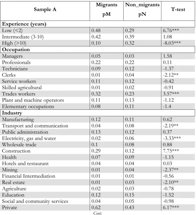
Table A1 presents a comparison of migrants versus non-migrants: columns two and three provide the proportion of people belonging to the different categories in the two sub-groups (pM and pN), while an analysis of the statistical difference of the two is provided in the last column. The individual details are taken from sample B (which is more complete as it includes the other one), while the occupational details are extracted from sample A. The purpose of the analysis is to identify distinctions between migrants and non-migrants and to put emphasis on the characteristics of the two groups. It is commonly believed that the migrant population is not randomly selected from the sample, which means that there are idiosyncratic elements that are marking the group (Greenwood, 1997). Non-parametric t-tests confirm this hypothesis since, among the personal details, most of the categories show a distinct pattern between migrants and non-migrants.

important for the old than for the young, may discourage older people from migrating (Greenwood, 1975).

The educational attainments put another wedge between the two groups; the summary statistics show that migrants are more educated than non-migrants: nearly 20% of movers are university graduates or above, while among non-movers only 9% obtained these qualifications. In both sub-samples, the majority of people went to primary school, but there is 10 percentage point difference between the two groups. The higher educational attainment of migrants is consistent with the theory, which predicts that better educated individuals are more likely to migrate, as they face lower risk and lower uncertainty in migration. Moreover, education decreases the deterring effects of distance, which is another important element hindering migration (Greenwood, 1975).

Regarding the occupation characteristics of the two groups, it is not surprising that migrants are a less experienced category than non-migrants: 48% of movers compared to 29% of non-movers have less than two years experience. On the contrary, 33% of non-migrants compared to 11% of migrants have more than 10 years experience. According to Mincer and Jovanovic (1981), “the initially steep and later decelerating declines of labour mobility with working age are in large part due to the similar but more steeply declining relation between mobility and length of job tenure”. The theoretical justification for this behaviour is linked to the increasing firm-specific skills an individual gains, working for long time in a firm: as far as these components of human capital are not easily transferable, they create a sort of attachment to the firm, reducing the incentive for migrating.

4. Methodology

This paper provides a test of the Harris-Todaro approach at aggregate district level, estimating a migration equation, where the dependent variable is a dichotomous outcome, which captures the existence of internal migration flows within Albania (_Mij). The country comprised 36 different districts and all pair-wise flows from one region to the other have been encountered.

) w w ; u u f( 1)

Prob(M_ij = = ~_j −~_i ~_j −~_i i=1,.., 36 j=1,.., 36 [1]

The district level wages (w~) and unemployment (u~), included in the migration equation, are retrieved from a first stage wage and unemployment equations, estimated controlling for personal characteristics. In order to test the predictions of the human capital model of migration, the earning function and the unemployment function are estimated emphasizing the difference between migrants and non-migrants. If the human capital model is correct, the realization of economic gains from migration must appear in the wage and unemployment equations.

The first micro level regression adopts a Mincerian wage equation, augmented with individual characteristics (X) and 36 district dummies (D), where the latter capture the areas where the sample respondents lived at the time of the survey.

) D , X ( f W

Without imposing a common intercept effect among the observations, each district dummy is free to impact differently on the dependent variable and unobservable district fixed effects are controlled for. The estimated coefficients of the district dummies in equation (2) represent the ceteris paribus wage rates for each region (w~).

The second regression is an unemployment probit function, where the probability of being unemployed is a function of personal characteristics (X) and district dummy variables (D).

) ,D f(X 1)

Prob(u_i = = _{i i} i=1,.., n [3]

The ceteris paribus district unemployment rates (u~) are computed as Φ(γ_i), where γiis the estimated coefficient of the ith district dummy variable and Φis the Cumulative Density Function of a Standard Normal Distribution.

5. Empirical Work

5.1 The Wage Determination Process

The wage function is specified to include personal characteristics such as gender (G), age (A), education (E), experience (T), marital status (M), and other relevant information such as occupation (O) and industries variables (I).

i z i z z y i y l i l l k i k k j i j j i h i h h f i f f i i i D MIG M O I G T E A A W

ε

ζ

ϑ

ψ

λ

γ

ϕ

φ

δ

β

α

∑

∑

∑

∑

∑

∑

∑

In agreement with the literature following Mincer (1974), the standard semi-log function is used and the dependent variable is expressed as the natural logarithm of monthly wages. The gender variable is computed as a dummy, taking the value of one if the individual is male. Age is a continuous variable and measures the number of years from birth. Two experience variables are included: one captures a low level of experience (less than two years) and the other an intermediate level (from three to five years). Five education variables capture educational qualifications: secondary, two years of vocational schooling, five years of vocational schooling, university and post-graduate. The marital status variables define a married and a divorced status. For a detailed definition of the variables see Table A2.

The equation is augmented using a gender dummy to control for unequal treatment across gender groups; industry dummies to control for compensating differentials, monopolistic market power or different input intensity across industries; occupation variables for skill level effects and marital status variables to proxy for family background considerations. Controls are also included for private enterprises and urban residence.

In order to capture the effect of the migration status on income realization, dummy variables for migrants are introduced (MIG)2_{: the intercept dummy captures the}

location specific human capital, whereas the interaction dummies allow different returns to individual characteristics between movers and non-movers3_{. Finally, district dummy}

variables (D) are specified in the regression to capture unobservable district fixed effects.

5.1.1 Results

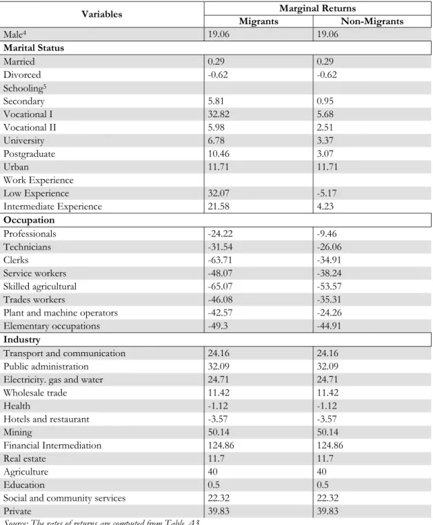
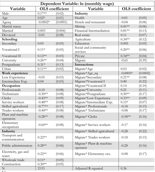
The ordinary least squares estimates are reported in Table A3 and robust standard errors are reproduced, using the variance-covariance matrix attributable to White (1980). Table 1 presents the rate of returns to the exogenous variables on monthly wages. As stated, the migration interaction terms capture the differences in potential earnings between movers and non-movers. Males enjoy higher wages than females: in fact a man, regardless of being migrant or a non-migrant, earns 19% more than a woman per month, on average and ceteris paribus, perhaps confirming the existence of some form of labour market discrimination. The highly insignificant coefficients of the marital status variables suggest that there is no significant difference in earnings between married, divorced and single persons.

Two results should be emphasized concerning the schooling variables: first of all, higher educational attainments have a strong impact on individual earnings, as proven by the statistically significant effect of the educational variables, and secondly migrants overall show higher returns to education than non-migrants, as suggested by the statistical effect of some of the interaction terms. For example, migrants who complete secondary schooling, on average and ceteris paribus, earn nearly six percent more than those who have only primary education or no education, whereas for non-migrants the rate of return to secondary education is 1% and this effect is not statistically significant. Moreover, a university postgraduate earns 10% more than a person with no education or primary education if he/she is a migrant and only three percent more if he/she is a non-migrant.

2 _{An attempt to control for international (return) migration was made, introducing dummy variables for}

those who stayed abroad for more than three months. This variable may capture the effect of new skills acquired abroad and brought home on earnings. However, the variable did not exert any effect on the wage and was therefore removed from the specification.

3 _{A testing down procedure was adopted to identify the final specification for estimation: starting from a}

Table 1: Rate of Returns for the Wage Equation - Migrants, Non-migrants (%)

Marginal Returns Variables

Migrants Non-Migrants

Male4 _{19.06 19.06}

Marital Status

Married 0.29 0.29

Divorced -0.62 -0.62

Schooling5

Secondary 5.81 0.95

Vocational I 32.82 5.68

Vocational II 5.98 2.51

University 6.78 3.37

Postgraduate 10.46 3.07

Urban 11.71 11.71

Work Experience

Low Experience 32.07 -5.17

Intermediate Experience 21.58 4.23

Occupation

Professionals -24.22 -9.46

Technicians -31.54 -26.06

Clerks -63.71 -34.91

Service workers -48.07 -38.24

Skilled agricultural -65.07 -53.57

Trades workers -46.08 -35.31

Plant and machine operators -42.57 -24.26

Elementary occupations -49.3 -44.91

Industry

Transport and communication 24.16 24.16

Public administration 32.09 32.09

Electricity. gas and water 24.71 24.71

Wholesale trade 11.42 11.42

Health -1.12 -1.12

Hotels and restaurant -3.57 -3.57

Mining 50.14 50.14

Financial Intermediation 124.86 124.86

Real estate 11.7 11.7

Agriculture 40 40

Education 0.5 0.5

Social and community services 22.32 22.32

Private 39.83 39.83

Source: The rates of returns are computed from Table A3

4 _{The returns to dummy variables are computed applying the following formula:}

Rate of return= (Exp(β) –1))*100, where the β coefficients are those reported in Table A3.

5 _{The rate of returns to the educational category are computed as: (Exp(}β_{) -1)/n*100, where n is the}

The size of the estimated returns to a university qualification for migrants is in line with the results obtained for other transitional economies (see for example Newell and Reilly, 1999), whereas it seems that non-migrants’ returns to university qualification is quite low, placing Albania among those countries that have the lowest rewards.

A common finding of the empirical literature is that individual heterogeneity plays a strong role in income realization: in fact, embodied in the human capital variables such as education and experience, there can be other elements, such as ability, motivation and the so-called D-factor (drive, dynamism, doggedness and determination) that positively affect earnings, but that cannot be observed and measured. Moreover, there might be differences that arise from the socio-economic background that cannot be captured. I am aware that if the direction of the correlation between the unobserved variables and earnings is positive, the coefficients of the human capital variables are biased upward.

Living in an urban area has a strong impact on earnings: on average and ceteris paribus those who live in cities earn 12% more than people resident in the rural areas. One possible explanation is the existence of compensating differentials for lower living costs and more pleasant environment enjoyed in the rural area. Moreover, trade unions may be more widespread in the urban areas than in the rural one and this has a relevant impact on wage levels and therefore on the incentive to migrate.

Among migrants, less experienced individuals show higher earnings than more experienced persons: a migrant with less than two years employment and a migrant with intermediate working years enjoys respectively 32% and 22% higher earnings than a migrant with more than 10 years employment. In the non-migrant category, on the other hand, experience seems to exert a weak impact on earnings, as proven by the statistically insignificant coefficients of the dummies. The empirical literature suggests that the impact of experience on earnings is positive and initially strong but the effect of additional years declines with the passage of time (Mincer, 1974). The explanation for this inverted U-shaped pattern is that “increased earnings are a reward for worker’s investment in implicit and explicit contracts” (Ehrenberg and Smith 1991) but in the long run “physical deterioration” can prevail. The fact that migrants show an opposite experience-wage pattern is not surprising: as long as migration is captured within the last 10 years, migrants do not have long attachments to their current job and didn’t develop strong firm specific experience. Migrants show higher returns to every experience classes than non-migrants: a possible explanation for these results can be due to the specific kind of training developed by movers; in fact they may have favoured a wide variety of jobs to a more firm specific attachment and according to Mincer (1974) “experience-earning profiles are steeper the smaller the proportion that is firm specific”.

Within non-migrants, the pattern of returns of different occupations are quite in line with what would be expected: managers are those who earn the most, while the less favoured group is the skilled agricultural labourers, who earn 54% less than the former category. For migrants the estimates would suggest a different story, with clerks the lowest-paid group together with skilled agricultural labourers. However, this result may be the consequence of small-cell bias, given the limited number of people belonging to the clerk category. The classification of the occupation category, however, is quite poor, as it hardly captures the skill differentials embodied in the available occupations.

showing the existence of industry wage differentials and strong regularities in the pattern of industrial premium (Krueger and Summers 1988) were highlighted. The estimated results (Table A3) confirm the hypothesis, as the coefficients are highly significant in many cases; the most advantaged category is the financial intermediation, as one would expect; compared to the base manufacturing group only health and hotels category show lower returns. It is surprising that the agricultural sector provides higher returns than the manufacturing one: an average employee in the agricultural sector earns wages that are 40 per cent higher than employees in the manufacturing industry. An explanation for the poor manufacturing performance may be linked to the liberalization of the economy, which negatively affected those sectors that lack competitiveness. Studying the industry wage differentials in U.S., Krueger and Summers (1988) report that the industry spreads ranged from a high of 37 per cent above the mean to a low 37 per cent below the mean. Even though the results of the U.S. study and those from Albania are not directly comparable, since in the former they normalize the estimated differentials as deviation from the weighted mean differential, a rough evaluation suggests that in Albania the spread is higher: the differentials vary from a 124 per cent above the base category to a four per cent below the base category. However, the spread might be overestimated, since it does not control for the weight each industry has on the total distribution. Moreover, because of the legacy of central planning, it is not surprising to discover a wider spread in Albania than in U.S, as a consequence of large productivity gaps among the investments.

Working as a private enterprise provides wages that are 40 per cent higher than working for a public owned institution, on average and ceteris paribus. The coefficient appears to be quite high for a transitional economy, even though the existence of a large and positive private premium was detected by the literature (for example, Reilly (2003) analysing the Serbian private sector, discovered an average wage premium of about 31% in 2000).

The age effect can be calculated from Table A3: the estimated age coefficient for migrants is 0.054, while the estimated age-squared coefficient is –0.00069. For non-migrants the coefficients are respectively 0.02 and –0.0002. The signs of these estimates suggest that wages increase with age, but at a decreasing rate, implying an inverted U-shape dynamic: this result is consistent with the human capital theory. The effect peaks when migrants are 39 years old and when non-migrants are 45 years old6_{, on average}

and ceteris paribus. The marginal effect of age (A) can be computed at average values and it results in 0.0026 for migrants and 0.0024 for non-migrants:

A) * *β (β

A wage

A_sq

a 2

ln

+ = ∂ ∂

( 7 ₎

This means that an additional year raises wages by 0.26 per cent for migrants and 0.24 per cent for non-migrants on average and ceteris paribus. The equality of the effects cannot be rejected by the data only marginally8_{. The results slightly confirm the}

findings of some studies on this literature: as Borjas (1987) wrote “the age-earnings

6 _{The value is derived taking the partial derivatives of log wage with respect to age. For migrants the}

maximum occurs at 39.13= 0.054/(2*0.00069), and for non-migrants at 45.04= 0.021/(2*0.00023).

7 _{The average age for migrants is 37, while for non-migrants is 40.}

profile of immigrants is steeper than the age-earnings profile of the native population with the same measured skills”.

Finally, the district wage rates were obtained introducing district dummy variables in the regression. Before calculating the values of the wage rate for each district, a Wald test was conducted in order to infer whether the data support district level effects on earnings: the hypothesis of one unique intercept among the 36 districts was rejected by the data9_.

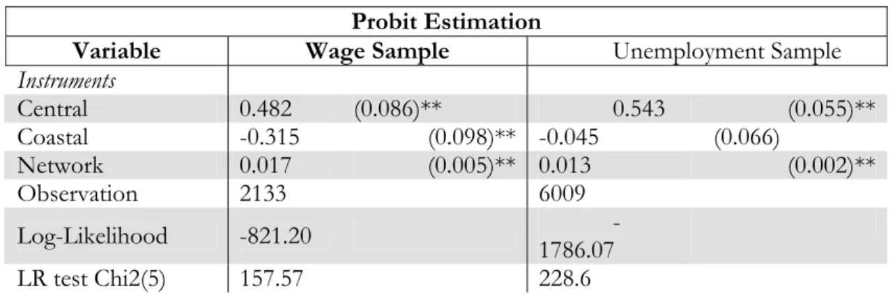
Economic theory suggests that there are important differences between migrants and non-migrants due to a self-selection mechanism: this concept refers to a process, which triggers people with some specific characteristics rather than others to migrate: if, for example, greater labour market ability and motivation raise earnings relatively more than they raise the costs of migration, the more able and the more motivated individuals will show a higher propensity to migrate (Chiswick,1978). From this follows that migrants might be endowed with different features than non-migrants and therefore they might not represent a random sample of the population; if the selection process is not taken into consideration, the estimated coefficients of an earning function can turn biased. Heckman (1976) offers a solution to correct for selectivity bias in a context of truncated sample. Empirically, there are some examples, which prove the existence of a self-selection mechanism: Robinson and Thomes (1982) find that both migrants and stayers are a self-selected category, although it is not possible to define a clear direction of the selection, whether positive or negative. Nakosteen and Zimmer (1980) find that migrants are not self-selected, whereas non-migrants result negatively self-selected.

In this paper a similar methodology is followed to test the existence of a self-selection process, and the results are reported in Appendix 2. The analysis rejects the hypothesis of self-selection in this data: this gives some confidence upon the unbiasedness of the estimated coefficients reported. The results are in agreement with other empirical examples, which failed to find self-selection: among others Hunt and Kau (1985), Axelsson and Westerlund (1998), Barham and Boucher (1998), Chiquiar and Hanson (2005).

Summarizing, two conclusions can be highlighted: the positive effect of internal migration on income, detected using the Albanian sample, gives support to the human capital theory; this theory in fact predicts that migration is an investment decision, or “an investment increasing the productivity of human resources” (Sjaasstad, 1962); the money returns to migration are expressed in terms of positive increment of the individuals’ earnings stream.

The second conclusion is that migrants may have lower location specific skills compared to non-migrant, which is suggested by the negative sign of the intercept dummy variable 10_{. This may be due to initially low knowledge of the local market and}

its opportunities, and/or lack of family networks and contacts which would help to find the best jobs available in the locality.

9 _{The Wald test gives Chi-squared (36)= 1576.}

5.2 The Unemployment Equation

The second step of the work requires the estimation of ceteris paribus district unemployment rates, retrieved from a micro level unemployment equation, which controls for individual characteristics. A probit model is used and the dependent variable represents the probability of being unemployed. The probit model to study unemployment has been extensively adopted in the literature (Nickell, 1979, 1980; Pissarides and Wadsworth, 1989, 1990; Brown and Session, 1996). The definition of unemployment follows the International Labour Organization (ILO) classification: unemployed are those who have no job but are actively looking for one. The employed group combines employees and the self-employed.

The covariates included in the equations are: age (A), education (E), gender (G), marital status (M) and urban residence (U).

∑

∑

∑

∑

i A E G M U MIG D

u

ob α β δ φ ϕ γ ξ υ [5]

To test the predictions of the human capital model in migration, the link between migration and unemployment status receives a distinctive attention: in particular, the key issue is whether being a migrant has a distinctive effect on the probability of being unemployed.

A first glance at the sample statistic (Table A1) would suggest that the influence of the migrant attribute is quite weak: in fact among non-migrants the proportion of unemployed is 12%, while among migrants, the proportion rises to 14%, but the difference is not statistically significant at conventional levels. Nevertheless, there might be some variables which distinguish migrants and non-migrants and which express an independent impact on the probability of being unemployed, requiring some interactive dummies (MIG)11_{. Finally, fixed regional effects are controlled for, through district}

dummy variables (D).

A brief comment is required: the problem of hidden employment is quite marked in transitional economies, which may suggest that the official estimates of the unemployment rate are mis-representing the real situation. In particular, among non-movers, the true unemployment rate may be lower than the one reported, which means that the available data are not able to capture potential differences in the unemployment likelihood between non-movers and movers.

5.2.1 Results

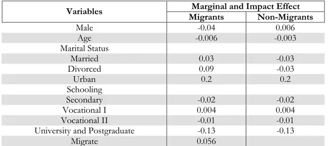
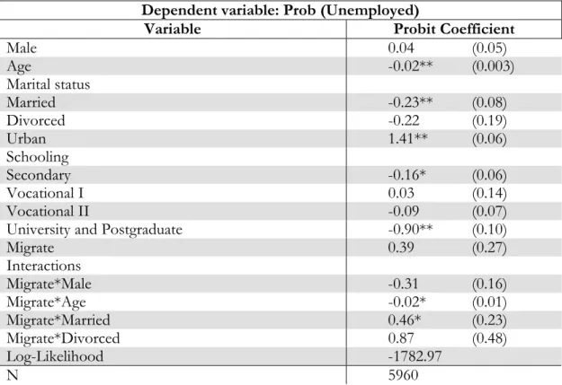
Maximum likelihood estimates are reported in Table A4, whereas Table 2 presents the estimated marginal and impact effects of the independent variables. A ceteris paribus analysis shows that a non-migrant male with average characteristics is about one percentage point more likely to be unemployed than a female, while within migrants, a male is four percentage points less likely to be unemployed than a female; however the coefficient of the male dummy is highly insignificant, while the coefficient of the

11 _{A testing down procedure again is adopted and it suggests interactive dummies for gender, age and}

interaction male dummy is significant at the 10 percent level. This result suggests that at least among non-movers there is not a marked gender division in the unemployment effect. This result confirms the findings in the general literature that gender differences in unemployment rates in most countries are small (Layard, Nickell and Jackman, 1991). The age coefficient shows that within both groups, young people are more likely to be unemployed, and the effect is more pronounced for migrants than non-migrants. In fact, in the first group an additional year decreases the probability of being unemployed by 0.6 of a percentage point, while for the second group the effect decreases to 0.3 of a percentage point. The theoretical explanations of this age-unemployment pattern are many: first “young workers are less able to acquire significant stocks of firm specific human capital by the time of downturn in demand” (Brown and Sessions, 1996); second they lack seniority and hence they are more vulnerable to job- dismissals and third, as the search theory would explain, they are more inclined to wait till they find the most suitable job, as they face lower forgone wages and long potential income streams to successful matches. Some authors (Brown and Sessions, 1996; Hughes and Hutchinson, 1988) were predicting a U-shaped relation between age and unemployment: the probability of being unemployed decreases until a certain age and it increases afterwards; since productivity is supposed to decline with age, older workers are more subjected to lay off. However, the sample data rejected this hypothesis, as an age-squared effect was poorly determined12_.

Table 2: Marginal and Impact Effects for the Probit Unemployment Function- Migrants, Non-migrants

Notes: See Table A2 for a full definition of terms. The marginal effects are computed from Table A4.

It is worth noting that the family background variables show an opposite impact on unemployment between migrants and non-migrants; within migrants, single people are the category less affected by unemployment: in fact, being married increases the probability by three percentage points and being divorced increases the probability by nine percentage points. On the contrary, for non-migrants married or divorced

12 _{Introducing the age-squared variable, both the age and the age-squared variables resulted in a}

non-significant effect (t-ratio age =0.025; t-ratio age squared= -1.338). On the contrary, without the age-squared variable, the age coefficient is highly statistically significant, as reported in Table A4.

Marginal and Impact Effect Variables

Migrants Non-Migrants

Male -0.04 0.006

Age -0.006 -0.003

Marital Status

Married 0.03 -0.03

Divorced 0.09 -0.03

Urban 0.2 0.2

Schooling

Secondary -0.02 -0.02

Vocational I 0.004 0.004

Vocational II -0.01 -0.01

University and Postgraduate -0.13 -0.13

individuals are less likely to be without a job. However only married people have a statistically different effect on unemployment compared to single persons. The theory is more in agreement with the non-movers’ results, predicting married individuals to be associated with the lowest risk of unemployment (Layard, Nickell and Jackman, 1991).

The urban variable presents a strong and well defined impact on the dependent variable; the effect is analogous for both groups: those living in the urban area compared to those residents in the rural area are 20 percentage points more likely to be unemployed. This result informs that in Albania unemployment is more an urban than a rural phenomenon.

The education estimates need a little discussion: it is surprising that a negative relationship between increasing educational attainment and unemployment is not well defined. In fact, compared to people with primary education or no education, those with two years of vocational education (Vocational I) are more inclined to be unemployed, even if the effect is not statistically different from zero. Five years of vocational education reduces the chance to be unemployed but again the effect is not well determined. On the contrary, secondary education reduces the probability of unemployment by two percentage points. This result suggests that professional schooling in Albania is not rewarded as much as secondary general schooling. University and postgraduate education exert a significant and strong impact on unemployment: a university degree or postgraduate studies ensure a 13 percentage points reduction in the probability of being unemployed. Nickell (1979) found a trade-off between the level of education and the probability of unemployment, confirming the assumption of the human capital model that education leads to the accumulation of human capital: the higher is the stock of human capital owned by a worker, the less firms are induced to lay him off. A little dissimilar are the findings of Brown and Sessions (1996): they discovered an inverse relationship between education and unemployment, but also some diminishing returns to education “with the largest reduction in risk occurring as we move from those respondents with non qualifications to those with minimal qualifications”. They also argue that in their study what probably matters is the achievement of a certain qualification threshold rather than a specific level of education.

It is worth calculating the ceteris paribus effect of being migrant, computed at average age13_{: a migrant at 35 years old is 5.6 percentage points less likely to be}

unemployed than a non-migrant.

Finally, the estimated coefficients of the district variables are used to compute the ceteris paribus district level rates relevant to study the migration function. It should be noted that a Log-Likelihood Ratio test was computed to test whether the data support a district level effects on unemployment: the data reject the hypothesis of one common intercept14_.

Concluding, the data reveal that migrants cannot be considered a distinct or less favoured category from non-movers: the coefficient of the migrant dummy is positive but not statistically significant (Table A4); four variables required interaction dummies,

13 _{The effect is calculated using the following formula:}

Age M

z

Age * M M z

2 1

2 1

β β

β β

+ = ∂

∂ + =

where the Greek letters represents the marginal effect estimates.

but a clear and easily interpretable justification for these interactions is not evident; the time spent in the host region resulted in a non significant effect on the probability of unemployment, suggesting that a longer time in the destination district does not provide any positive impact on the unemployment likelihood. Finally, the Heckman two step procedure has been applied (see Appendix 2) and the result suggests that neither migrants nor stayers are self-selected.

In conclusion it emerges that the distinction between migrants and non-migrants is quite frail, which confirms the findings of the descriptive data analysis (Table A1). However it is worth noting that the function adopted to model the likelihood of unemployment is quite austere: more explanatory variables would be necessary to give a more precise specification, but the limited availability of detailed personal and other information restricted the analysis.

5.3 The Migration Function

In the following section, the Harris-Todaro migration approach is tested: this theory treats differentials in economic opportunity, such as earnings, as the primary driving forces of reallocation. Moreover, in agreement with the model of Todaro (1969) and Harris-Todaro (1970), the hypothesis that agents respond to expected rather than real wages is tested.

The contribution of the human capital model in migration is as well taken into consideration: the human capital model emphasises the role of heterogeneity in economic realization and suggests that aggregate migration regressions are unable to capture the joint effect of human capital characteristics on earnings and migration decision. Only if the population is homogeneous, in fact, the estimated relationship resulting from a macro-level regression can represent the structural framework implied by the human capital model. Therefore, in order to control for individual heterogeneity, the wages and unemployment differentials, included in the aggregate migration equation, are retrieved from a first stage wage and unemployment equations, and represent the ceteris paribus district level rates. The previous analysis, in fact, led to the definition of 36 wage (w~) and unemployment (u~) rates, one for each Albanian district, computed controlling for personal and demographic factors.

The specification is a Probit function, where the dependent variable is a binary choice proxying for the propensity to migrate from region i to region j: in particular,

M=1 if there was a migration flow at any time after 1992 from district i to district j, and 0 otherwise; u~_jand w~_j are the destination rates, whereas u~_i and w~_i are the origin rates.

{

}

Φ 1)

Prob(M_ij = = ₁ + ₂ ~_j −~_i + ₃ ~_j − ~_i i=1,.., 36 j=1,.., 36 [6]

In the specification it is assumed that the origin and destination variables exert a symmetric but opposite effect on migration, in agreement with other studies in the empirical literature (see for example Schultz, 1982).

confirmed by the empirical literature, which analyses the speed of adjustment of economic variables toward the equilibrium. As stated in Greenwood (1997) and Zimmermann (1995), the process of convergence can be quite slow and it depends on the rigidity of the economic variables, due to social and institutional barriers. The existence of a slow convergence mechanism and of high rigidities of the economic variables can be quite plausible in Albania, as a heritage of the former central planning system.

5.3.1 Results

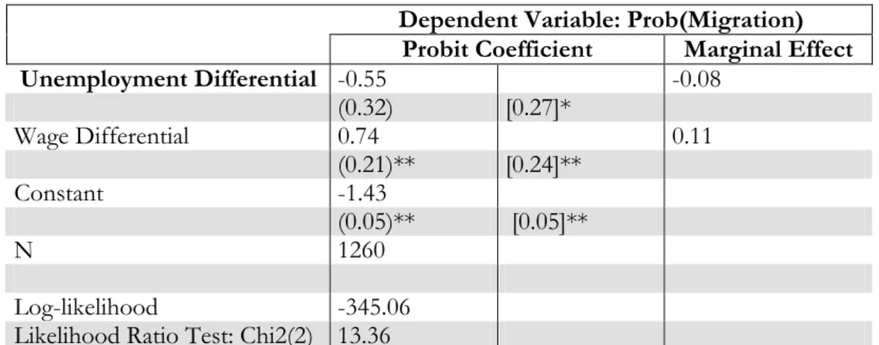
Table 3 presents the maximum-likelihood estimates of the migration equation and the marginal effects. The probit model appears to fit the data on internal migration quite well: in fact, the Log-Likelihood Ratio test indicates that the overall relation is significant at the five percent level and both the unemployment differential and the wage differential are able to explain the flow of migration. The estimated relationship is in the expected direction: higher earning gaps boost migration, whereas higher unemployment gaps deter emigration.

Table 3: Propensity to Migrate Estimates- Probit Regression

Dependent Variable: Prob(Migration) Probit Coefficient Marginal Effect

Unemployment Differential -0.55 -0.08

(0.32) [0.27]*

Wage Differential 0.74 0.11

(0.21)** [0.24]**

Constant -1.43

(0.05)** [0.05]**

N 1260

Log-likelihood -345.06 Likelihood Ratio Test: Chi2(2) 13.36

Notes: The standard errors are given in round brackets, and bootstrapped standard errors are given in squared brackets. Dependent variable= binary choice, taking the value of 1 if a migration flow is observed, 0 otherwise.** denotes statistical significance at 1% level, *denotes statistical significance at 5% level using two tailed tests.

The wage coefficient of the model suggests that, on average and ceteris paribus, an infinitesimal change in the wage differential between destination and origin raises the probability of observing a migration flow by 11 percentage points. The unemployment coefficient suggests that a marginal increase in the unemployment gap reduces the probability of migration by eight percentage points.

It should be noted, that when generated variables appear in a regression equation, the OLS estimated variance is generally inconsistent, invalidating inferential analysis on the coefficients (Pagan, 1984). To correct the estimated standard errors, a nonparametric bootstrap method was applied15_.

15_{The number of replications performed in Stata is 200. Mooney and Duval (1993) show that 200}

In the empirical literature, many examples provide support to the positive link between earning differentials and migration; on the contrary, the relationship between migration and unemployment rates is still quite dubious. Among aggregate level analysis, Schultz (1982) finds that wage differentials are important determinants of regional migration in Venezuela. Todaro (1980) compares the findings of similar macro-level studies and concludes that “wage levels between two places turn up among the most important explanatory factors”. In Finland, Eriksson (1988) reports a positive impact of regional wage differentials and a negative impact of regional unemployment ratios on net migration rates.

Falaris, (1979) finds that for Peru only earnings at destination have a significant (positive) effect on migration, whereas employment-rate coefficients at origin and destination are not significant. Analyzing international migration, Karemera et al. (2000) report positive elasticities of emigration flows to US with respect to destination country income and negative elasticities with respect to origin countries GDP; on the contrary, emigration flows do not respond to unemployment rates. Mayda (2005), extending the analysis to a multitude of origin and destination nations, supports the findings that destination country GDP exerts a positive impact on emigration rates, whereas the effect is reversed with respect to origin country income. Faini and Venturini (1994) report that emigration rates for south European countries are influenced by wage differentials, by unemployment rates in destination countries and only marginally by unemployment rates in origin countries; however, the most interesting result is that the level of income in origin countries has a non-linear effect on emigration: in particular growth boosts migration for poor countries, whereas it depresses emigration in relatively richer nations.

Some micro-level studies can be quoted: Nakosteen and Zimmer (1980) and Robinson and Tomes (1982) find that earning differentials positively impact on individual probability of migrating. Lucas (1985) concludes that the propensity to migrate increases with higher wages in destination urban areas and it decreases with higher home village wages; moreover, the lower (higher) the chance to be unemployed at destination (origin) the higher the probability of emigration. Finally Herzog et al. (1993), presenting a survey of the empirical literature based on US data, report that four out of eight studies find that both the unemployment rate and the wage rate are a significant determinant of out-migration.

6. Comparative Remarks for transition countries

The centrally planned economic system ensured full employment and relatively equalized incomes among social groups and among regions, by means of subsidies, transfers and controlled prices. The transition to a market economy, however, introduced large regional disparities in income levels and unemployment rates. The existence of such differentials produced the economic incentives to migrate not only for Albanians but also for the citizens of the entire block of the newly independent states of the former Yugoslavia and of the countries originated on the ground of the former URSS. This situation generated a great interest in the analysis of interregional migration in transition countries, which stimulated a vast empirical literature.

disparities, despite the existence of large economic differentials. Nevertheless, economic motives remain strong determinants of migration.

In Czech Republic, Hungary, Slovakia and Poland migration is found to depend on wages and unemployment, but the pattern is not fully consistent with the predictions of the economic theory. In fact, high wages encouraged not only high immigration, but also high emigration; at the same time, regions with high unemployment experience not only low inbound but also low outbound. This implied that high migration, both inbound and outbound, affected only the relatively prosperous regions, whereas the most depressed ones experienced a very limited labour mobility, creating persistence in regional economic gaps (Fidrmuc, 2004).

A correlation analysis for Czech Republic, Hungary, Poland, Romania and Russia indicates that net migration is larger in regions with lower unemployment and higher per capita incomes (Bornhorst and Commander, 2004). Despite low unemployment and high relative wages represent strong motives to migrate, internal migration remained quite limited in these countries.

Low responsiveness of migration to wage and unemployment differentials in Czech Republic and Slovenia is reported as well in Huber (2004). The estimation displays insignificant coefficients for wage gaps and a significant parameter for unemployment rates only for Czech Republic.

In Russia overall migration during the transition period remained quite limited, but economic motives are the main engine of interregional mobility. Migration flows are driven by poor economic conditions in source regions and by high incomes in destinations. It is as well influenced by the unemployment rate in the destinations (Andrienko and Guriev, 2004).

Boeri and Scarpetta (1996) associate the inelastic response of migration in transition countries to uncertainty for the future and to the increasing costs of mobility due to limited rental housing. Moreover, migration flows have a pro-cyclical pattern, and this explains why net migration was low during the dramatic downturn which characterized the economic transition.

7. Summary and Conclusions

The primary purpose of this research is to study the determinants of internal migration in Albania. Moreover, in order to control for the heterogeneity of the population, the cross-region propensity to migrate has been explained by ceteris paribus

inter-district differentials, retrieved from a first stage wage and unemployment functions. The inclusion of ceteris paribus measures, rather than average ones, reflects insights from the human capital model in migration, that individuals display different propensity to migrate, because of the different remuneration the human capital characteristics have in alternative locations. Controlling for personal characteristics and district-level effects, unemployment and wage functions have been estimated, emphasizing the distinction between migrants and non-migrants: this has been done to detect any significant positive effect of migration on earnings and on the likelihood of unemployment.

to the human capital theory, which predicts that individuals invest in migration to enjoy greater economic opportunities. Movers choose destinations where the returns to their personal characteristics are maximized. Moreover a lower location specific skills of migrants compared to non-migrant was detected.

The interpretation of the results in the unemployment function is more ambiguous and direct support for the human capital theory is not obtained. The distinction between migrants and non-migrants is quite frail, but it may be attributable to a rather austere specification of the model adopted to the test the likelihood of unemployment.

Some studies that focused on migration, detected the existence of a selectivity mechanism: if this mechanism works in the migration process and it is not taken into account, the estimated coefficients of the equations may be biased. However it seems that this problem was not affecting the sample used in this analysis.

It is worth noting that aside from a migration analysis issue, the wage and unemployment functions provide interesting and well defined results. This first attempt to analyse a wage determination process and an unemployment function in Albania, offers encouraging outcomes: the estimated coefficients are well defined in most of the cases and they are in line with what the theory predicts.

Employing aggregate data, the migration probit function confirmed the role of economic variables in the migration decision. The results reveal that not only wage but also unemployment differentials are important explanations for the propensity to migrate: a marginal increase in the wage gap between destination and origin raises the probability of observing migration within the districts by 11 percentage points, on average and ceteris paribus. The same variation in the unemployment gap raises the probability by 8 percentage points.

Finally the analysis on the reasons to migrate corroborates the previous results, namely the importance of economic factors in the migration decision: job related aspects, such as wage, new opportunities and also the search of better quality land are primary pushing factors, though not exclusive; these determinants, moreover, gain increasing importance at higher level of education.

References

Andrienko Y. and S. Guriev (2004), ‘Determinants of interregional mobility in Russia’, Economics of Transition, 12, 1-27

Axelsson R., Westerlund O. (1998), ‘A Panel Study o Migration and Household Real Income’, Journal of Population Economics, 11, 113-126

Barham B., Boucher S. (1998), ‘Migration, Remittances and Inequality: Estimating the Net Effects of Migration on Income Distribution’, Journal of Development Economics, 55(2), 307-331 Bauer T. , Zimmermann K. (1999), ‘Causes of International Migration’ in Gorter C., Nijkamp P.

and Poot J. (eds), Crossing Borders: Regional and Urban Perspectives on International Migration, Ashgate, Aldershot

Boeri T. and S. Scarpetta (1996), ‘Regional mismatch and the transition to a market economy’, Labour Economics, 233-254

Borjas G.J. (1987), ‘Self-selection and the earnings of immigrants’, The American Economic Review, 77(4), 531-553

Bornhorst F. and S. Commander (2004) ‘Regional Unemployment and its Persistence in Transition Countries’, IZA Discussion Paper 1074, IZA Bonn

Brown S., Sessions G. (1996), ‘A profile of the UK Unemployment: Regional versus Demographic Influences’, Regional Studies, 31(4), 351-366

Chiquiar D., Hanson G. (2005), ‘International Migration, Self-Selection and the Distribution of Wages: Evidence from Mexico and United States’, Journal of Political Economy, 113(2), 239-281 Chiswick B. R. (1978),’The effect of Americanization on the Earnings of Foreign-born Men’,

The Journal of Political Economy, 86(5), 897-921

Clark X., Hatton T.J., Williamson J.G. (2002), ‘Where Do US Immigrants Come From, and Why?, NBER Working Paper n.8998, National Bureau of Economic Research, Cambridge Ehrenberg R.G., Smith R.S. (1991), Modern Labour Economics: Theory and Public Policy, Harper

Collins Publisher

Eriksson T. (1988), ‘International Migration and Regional Differentials in Unemployment and Wages: Some Evidence from Finland’, in Gordon I. and Thirwall A. (eds), A European Factor Mobility, Trends and Consequences, MacMillan, Hampshire and London.

Faini R., Venturini A. (1994), ‘Migration and Growth: The Experience of Southern Europe’, CEPR Discussion Paper n. 964, Centre For Economic Policy Research, London

Falaris E.M. (1979), ‘The determinants of Internal Migration in Peru: An Economic Analysis’, Economic Development and Cultural Change, 27, 327-341

Fidrmuc (2004), ‘Migration and Regional Adjustment to asymmetric shocks in transition economies’, Journal of Comparative Economics, 32, 230-247

Greenwood M.J. (1975), ‘Research on Internal Migration in the United States: A Survey’, Journal of Economic Literature, 13(2), 397-433

Greenwood M.J. (1997), ‘Internal Migration in Developed Countries’, in Rosenzweig M.R., Stark O. (eds), Handbook of Population and Family Economics, Elsevier Science B.V.

Heckman J.J. (1976), ‘The common structure of statistical models of truncation, sample selection and limited dependent variables and a simple estimator for such models’, Annals of Economics and Social Measurement, 5, 475-492

Herzog H.W., Schlottmann A.M., Boehm T.P (1993), ‘Migration as Spatial Job-search: a Survey of Empirical Findings’, Regional Studies, 27(4), 327-340

Huber P. (2004), ‘Intra-national labor market adjustment in the candidate countries’, Journal of Comparative Economics, 32, 248-264

Hughes P.R., Hutchinson G. (1988), ‘Unemployment, Irreversibility and the Long-term Unemployed’, in Cross R. (eds), Unemployment, Hysteresis and the Natural Rate Hypothesis. Blackwell, Oxford

Hunt J.C., Kau J.B. (1985), ‘Migration and Wage Growth: A Human Capital Approach’, Southern Economic Journal, 51, 697-710

Karemera D., Oguledo V.I., Davis B. (2000), ‘A Gravity Model analysis of International Migration’ Applied Economics, 32, 17445-1755

Krueger A.B., Summers L.H. (1988), ‘Efficiency Wages and the Inter-Industry Wage Structure’, Econometrica, 56(2), 259-293

Layard R., Nickell S., Jackman R. (1991), Unemployment: Macroeconomic Performance and Labour Market, Oxford University Press, Oxford

Lucas R.E.B. (1985), ‘Migration amongst the Botswana’, The Economic Journal, 95(378), 358-382 Lucas R.E.B. (1997), ‘Internal Migration in Developing Countries’ in Rosenzweig M.R., Stark O.

(eds), Handbook of Population and Family Economics’, Elsevier Science B.V.

Mayda A. M. (2005), ‘International Migration: A Panel Data Analysis of Economic and Non-Economic Determinants’, IZA Discussion Paper n.1590, IZA Bonn

Mincer J. (1974), Schooling, Experience and Earnings, New York: National Bureau of Economic Research.

Mincer J. (1978), ‘Family Migration Decision’ TheJournal of Political Economy, 86(5), 749-773 Mincer J., Jovanovic B. (1981), ‘Labour Mobility and Wages’, in Rosen S. (eds), Studies in Labour

Markets, The University of Chicago Press

Mooney C.Z., Duval R.D. (1993), Bootstrapping: a Nonparametric Approach to Statistical Inference, Newbury Park, Sage Publications

Nakosteen R.A., Zimmer M. (1980), ‘Migration and Income: the Question of Self Selection’, Southern Economic Journal, 46, 840-851

Newell A., Reilly B. (1999), ‘Rates of Returns to Educational Qualifications in the Transitional Economies’, Education Economics, 7(1), 67-84

Nickell S. (1979), ‘Education and Lifetime Patterns of Unemployment’, The Journal of Political Economy, 87(5), S117-S131

Nickell S. (1980), ‘A picture of male unemployment in Britain’, Economic Journal, 90, 776-794 Pagan A. (1984), ‘Econometric Issues in the Analysis of Regressions with Generated

Regressors’, International Economic Review, 25(1), 221-247

Pissarides C.A., McMaster I. (1990), ‘Regional Migration, Wages and Unemployment: Empirical Evidence and Implications for Policy’, Oxford Economic Papers, 42(4), 812-831

Pissarides C.A., Wadsworth J. (1989), ‘Unemployment and the Inter-Regional Mobility of Labour’, The Economic Journal, 99(397), 739-755

Reilly B. (2003), ‘The Private Sector Wage Premium in Serbia (1995 – 2000): A Quantile Regression Approach’, University of Sussex Discussion Papers in Economics n. 98

Robinson C., Tomes N. (1982), ‘Self-Selection and Interprovincial migration in Canada’, Canadian Journal of Economics, 15, 474-502

Schultz T.P. (1982),’Lifetime Migration within Educational Strata in Venezuela: Estimates of Logistic Model’, Economic Development and Cultural Change, 30, 559-593

Sjaastad L.A. (1962), ‘The Costs and Returns of Human Migration’, The Journal of Political Economy, 70(5), 80-93

Stacher I., Dobernig I.P. (1997), ‘Migration in Central and Eastern Europe, Compilation of National Reports on Recent Migration Trends in the CEI States’ ICMPD, Vienna

Todaro M.P. (1969), ‘A model of Labour Migration and Urban Unemployment in Less Developed Countries’, American Economic Review, 59(1), 138-148

Todaro M.P. (1980), ‘Internal Migration in Developing Countries: A Survey’, in Easterlin R.A. (eds), Population ad Economic Change in Developing Countries, NBER, Chigago.

UN (2002), ‘Common Country Assessment, Albania’, Prepared for the United Nation System in Albania by the Albanian Center for Economic Research (ACER)

Vella F. (1998), ‘Estimating Models with Sample Selection Bias: A Survey’, The Journal of Human Resources, 33, 127-169

White H. (1980), ‘A Heteroscedasticity-Consistent Covariance Matrix Estimator and a Direct Test for Heteroscedasticity’, Econometrica, 48, 817-838

World Bank (2003), ‘Albania Poverty Assessment’, Human Development Sector Unit, Report n.26213-AL, The World Bank, Washington DC

Appendix 1

Table A1: Summary Statistics and Tests for Differences in Means

Sample A Migrants

pM

Non_migrants

pN T-test

Experience (years)

Low (<2) 0.48 0.29 6.76***

Intermediate (3-10) 0.42 0.39 1.08

High (>10) 0.10 0.32 -8.03***

Occupation

Managers 0.05 0.03 1.58

Professionals 0.22 0.22 0.11

Technicians 0.09 0.12 -1.37

Clerks 0.01 0.04 -2.12**

Service workers 0.11 0.12 -0.42

Skilled agricultural 0.01 0.02 -0.91

Trades workers 0.32 0.23 3.57***

Plant and machine operators 0.11 0.13 -1.12

Elementary occupations 0.08 0.11 -1.4

Industry

Manufacturing 0.12 0.11 0.62

Transport and communication 0.04 0.08 -2.19**

Public administration 0.13 0.12 0.37

Electricity, gas and water 0.02 0.06 -3.33***

Wholesale trade 0.1 0.08 0.88

Construction 0.29 0.12 7.75***

Health 0.07 0.09 -1.15

Hotels and restaurant 0.04 0.04 0.03

Mining 0.01 0.04 -2.37**

Financial Intermediation 0.01 0.01 -0.56

Real estate 0.01 0.03 -2.10**

Agriculture 0.02 0.03 -0.78

Education 0.12 0.15 -1.52

Social and community services 0.04 0.05 -0.98

Private 0.62 0.43 6.17***

Sample B Migrants pM

Non_migrants

pN T-test

Male 0.53 0.57 -1.84*

Age group

< 25 0.18 0.2 -0.99

26-36 0.35 0.24 5.89***

37-50 0.35 0.4 -2.15**

>50 0.12 0.16 -3.08***

Education attainment

No schooling 0.01 0.01 -0.39

Primary 4 years 0.04 0.07 -3.01***

Primary 8 years 0.42 0.49 -3.19***

Secondary General 0.16 0.17 -0.58

Vocational I (2 years) 0.02 0.02 -0.9

Vocational II (4 years) 0.16 0.14 1.28

University 0.18 0.09 7.24***

Postgraduate 0.01 0.004 2.54**

Family status

Married 0.83 0.75 4.12***

Divorced 0.02 0.02 0.15

Single 0.15 0.23 -4.31***

Unemployed 0.14 0.12 1.47

Urban 0.67 0.43 11.14***

Notes:

*** denotes statistical significance at 1% level. **denotes statistical significance at 5% level .

* denotes statistical significance at 10% level using two tailed tests. The proportions are calculated for migrants and non-migrants separately. To receive 100% one should add vertically the proportions within each group of variables.

The non-parametric t-test is computed as:

[

] [

]

NM

M p / p(1 p)/n p(1 p)/n

p − − + −

where pM and pNM represents, respectively, the proportion of migrants and non-migrants in each category; p represents the fraction of individuals in each category: it is computed as the sum of the absolute number of migrants and the absolute number of non-migrants for each category divided by the total number of people in the sample.

M