Surfaces with Prescribed Nodes and Minimum Energy Integral of Fractional Order

(1)

Surfaces with Prescribed Nodes and Minimum Energy

Integral of Fractional Order

H. Gunawan1, E. Rusyaman2 & L. Ambarwati1,3

1_{Analysis and Geometry Group, Faculty of Mathematics and Natural Sciences, Bandung}

Institute of Technology, Bandung, Indonesia.

2

Department of Mathematics, Padjajaran University, Bandung, Indonesia.

3_{Department of Mathematics, State University of Jakarta, Jakarta, Indonesia}

Email: [email protected]

Abstract. This paper presents a method of finding a continuous, real-valued,

function of two variables zu x y( , ) defined on the square 2 : [0,1]

S  , which minimizes an energy integral of fractional order, subject to the condition u(0, )y 

(1, ) ( , 0) ( ,1) 0

u y u x u x  and u x y( ,_i _j)c_ij, where 0x₁ ... xM 1,

1

0y  ... yN 1, and 𝑐 ∈ ℝ are given. The function is expressed as a

double Fourier sine series, and an iterative procedure to obtain the function will be presented.

Keywords: 2-D interpolation; energy-minimizing surfaces.

1 Introduction

In [1], A.R. Alghofari studied the problem of finding a sufficiently smooth function on a square domain that minimizes an energy integral and assumes specified values on a rectangular grid inside the square. In particular, he discussed the existence and uniqueness of a solution to the problem, using tools in functional analysis and calculus of variations. The problem is related to the analysis of satellite data, which is important and useful from the application point of view.

In this paper, we shall discuss a method of finding a continuous, real-valued, function of two variables z= ( , )u x y defined on the square 2

:= [0,1]

S , which minimizes the energy integral

1 1 ₂

2 0 0

( ) := | ( ) | ,

E u u dxdy



 



subject to the condition u(0,y)=u(1,y)=u(x,0)=u(x,1)=0 and u x y( ,_i _j) =c_ij,

(2)

Laplacian on ℝ2, and ₍ ₎2





 (with



0) is its fractional power --- which will be defined soon. For =2, E_(u) represents the (total) curvature or the strain energy on

S

(see [2]).

Using real and functional analysis arguments, we show that such a function exists and is unique if and only if >1. The function may be expressed as a double Fourier sine series. As in [3], we also provide an iterative procedure to obtain the function, and explain how it works through an example.

Related works may be found in [4,5]. Applications of energy-minimizing surfaces may be found in [6-8] and the references therein.

2 The Existence and Uniqueness Theorem

We shall here show that given

M



N

points ( ,x y_i _j) with

1 <

<

0 x

₁



x

_M ,

0 <

y

₁

<



<

y

_N

<

1

, and

M



N

values 𝑐 ∈ ℝ, there exists a function z=u(x,y) such that (i) u(0, ) = (1, ) =y u y

( , 0) = ( ,1) = 0

u x u x , (ii) u(x_i,y_j)=c_ij for i=1,,M , j=1,,N, and (iii) the energy integral E_(u) is minimum. The continuity of the function will depend on the value of , which we shall see later.

As we are working with functions uon S=[0,1]2 that vanish on the boundary, we may represent u as a double Fourier sine series

, =1

( , ) =

_mn

sin

.sin

.

m n

u x y

a

m x



n y







Since the boundary condition (i) is already satisfied, we only need to take

care of the other two conditions.

The fractional power of



_{is defined as follows. Computing}

2 2 2 2

= u u

u

x y

 

  

 

, we obtain

2 2 2

, =1

( , ) = ( ) _mnsin .sin .

m n

u x y  m n a m x n y









As in [9], for 0, we define the fractional power ₍ ₎2 

(3)

y n x m a n m y x u _mn n m          

 ( ) sin .sin

:= ) , ( )

( 2 2 2

1 = , 2

Thus, if u is identified by the array of its coefficients

[

a

_mn

]

, then ₍ _{) u}2 

 is

identified by the array _[ ₍ 2 2₎2 _]

mn

m n a

 



 . One may observe that the formula matches the computation of the nonnegative integral power of , that is,

when



= 2 ,k k= 0,1, 2,. [Note also that ₍ _{) (}2 _{) = (}2 ₎ 2    

  

for

every

 

, 0

.]

With the above definition of ( )2 



 , the energy integral E_(u) may now be given by the sum

2

2 2 2

, =1

( ) =

(

) .

4

m n mn

E u

a

m

n

  









Thus our problem can be reformulated as follows: find a continuous, real-valued, function of two variables zu x y( , ) defined on the square

S

: [0,1]



2 , which minimizes the energy integral

2

2 2 2

, =1

( ) =

(

) .

4

m n mn

E u

a

m

n

  









subject to the condition u(0, )y u(1, )y u x( , 0)u x( ,1)0 and

( ,i j) ij

u x y c , where

0   

x

₁

...

x

_M



1

,

0 

y

₁

 

...

y

_N



1

and 𝑐 ∈ ℝ are given. Here u is identified by

[

a

mn

]

, and the problem is to determine the value of

a

_mn's such that the prescribed values c_ij are assumed at (x_i,y_j) and the latest sum is minimized.

(4)

Let us now turn to how to solve the problem. Denote by W =W_ the space of

all functions

, =1

( , ) = _mnsin sin

m n

u x y a m x n y





for which 2 2 2 , =1

( ) <

mn m n

a m n 



 



--- our admissible functions. On

W

, we define the inner product , by 2 2

, =1

,

:=

_{mn mn}

(

) ,

m n

u v

a b

m

n













where

a

_mn's and

b

_mn's are the coefficients of u and v respectively. Its induced norm is

1 2

2 2 2

, =1

:=

_mn

(

)

.

m n

u

a

m

n





















Then we have the following fact, whose proof is routine, and so we leave it to the reader.

Fact 2.1 (W,,)is a Hilbert space.

For >1, we have the following result.

Theorem 2.2 Let >1. If

(

u

_k

)

converges to u in norm, then ₍ ₎2

k

u





converges to ₍ ₎2u





 uniformly, whenever 0

 

< 1. In particular, if

)

(

u

k converges to u in norm, then

(

u

k

)

converges to u uniformly.

Proof. Let amn( )k 's and

a

mn's be the coefficients of

u

k and u respectively, and

0

 

< 1. Then, for every ( , )x y S, we have

 



 





 



_

_

2 2

2 2 ₂ ( ) , 1 1 1 2 2 2 2 2 2 2 ( )

2 2

, 1 , 1

( , ) ( , ) sin sin sin sin . k k mn mn m n k mn mn

m n m n

u x y u x y

m n a a m x n y

m x n y

m n a a

(5)

Let us now have a closer look at the last expression on the right hand side. The first sum is nothing but u_k u 2. The second sum is dominated by

2 2 , =1

1 ( )

m n m n

 



 



. Since >1, this sum is convergent (by the integral test). Hence, we find that

2 2

| ( ) u x y_k( , ) ( ) u x y( , ) | C u_k u ,

 

    

where

C

is independent of ( , )x y . This shows that ₍ ₎2

k

u



 converges to

2 ( ) u



 uniformly, as desired.

□

Corollary 2.3 Let >1. Then, every function

u



W

is continuous on

S

.

Proof. If

u



W

, then u is a limit (in norm), and hence a uniform limit, of the partial sums

u

a

mn

m

x

n

y

k

n k

m

k

:=

 

sin



sin



1 = 1 =

. Since the partial sums are

continuous on

S

, then u too must be continuous on

S

. □ To prove the existence and uniqueness of the solution to our problem, we define

:= { : ( ,i j) = ij, = 1, , , = 1, , }

U uW u x y c i  M j  N

and

:= { : ( ,_i _j) = 0, = 1, , , = 1, , }.

V uW u x y i  M j  N

Then, as in [1], we have the following fact.

Fact 2.4

U

is a non-empty, closed, and convex subset, while

V

is a closed subspace of

W

.

Proof. We shall only prove that

U

is non-empty, and leave the others to the reader. Consider the system of linear equations

=1 =1

sin sin = , = 1, , , = 1, , .

M N

mn ij

m n

a m x



n y



c i M j N

(6)

The system will have a solution if the matrix

1 1 1

1 1 2

sin [sin ] sin 2 [sin ] sin [sin ]

:= ,

sin [sin ] sin 2 [sin ] sin [sin ]

i i i

N i N i N i

y m x y m x N y m x

A

y m x y m x N y m x



 

 

 

 

   



is non-singular. The matrix A is the Kronecker product of the nn matrix

n j j

j n y

y

n ]:=[sin ] _,

sin

[   and the mm matrix [sinm x _i]:= [sinm x i i m]_, . Hence, we obtain

det

A

= (det[sin

n y



_j

])

m



(det[sin

m x



_i

])

n

(

see [10]). Since [sinn y j] and [sinm x i] are both non-singular (see, for

example, [11]), we conclude that the matrix A is non-singular too. Therefore

the above system of equations has a solution, which means that

U

is non-empty.

□

The existence and uniqueness of the solution to our problem follows from the best approximation theory in Hilbert spaces.

Theorem 2.5 The problem has a unique solution in

W

, and the solution is given by

0 0

:=

proj ( )

_V

u



u

for any choice

u

₀



U

. Furthermore, for >1, the function u is continuous on

S

.

Proof.

Take an element

u

₀ in

U

. Then, for any

v V



,

u

₀



v

is also in

U

. Since

U

is a convex subset of

W

, there must exist a unique element

v

₀



V

such that

u

₀



v

₀ is minimum [12]. Thus

u

:=

u

₀



v

₀ is the unique solution in

W

_{for our minimization problem. By the best approximation theory in Hilbert}

spaces, the element

v

₀



V

that minimizes

u

₀



v

₀ must be the orthogonal projection of

u

₀ on

V

, that is,

v

₀

= proj ( )

_V

u

₀ . The solution is independent of the choice of

u

₀



U

. Indeed, if

u u

₀

,

₁



U

, then

u

₀

 

u

₁

V

, and so



0 1



0 1

(7)

In the next section, we shall discuss how we actually find the solution to our problem.

3 The Procedure to Find the Solution

To find an element

u

₀ in

U

is easy, we only need to solve the system of linear equations

=1 =1

sin sin = , = 1, , , = 1, , .

M N

mn ij

m n

a m x



n y



c i M j N



 

Here

u

₀ can be thought of as an initial approximation to the solution we are looking for. Once we have

u

₀, we just have to compute its orthogonal projection on the subspace

V

.

To do so, we first determine an orthogonal basis of

V

. We note that every element of

V

must satisfy

=1 =1 ,

sin

=

sin

,

M N

mn i j mn i j

m n m n

a

m x



n y





a

m x



n y







for i=1,,M, j=1,,N, where the sum on the right hand side is taken over m and n with “

m



M



1

or

n



N



1

”. From this, we may basically express

a

_mn for m=1,,M,n=1,,N in terms of

a

_mn with “

m



M



1

or

n



N



1

”. Thus, every element of

V

may be written as ,

= _{mn mn},

m n

v



a v

for some elements

v

_mn in

V

. [For >1, one may check that the subspace

V

has co-dimension

M



N

.]

(8)

* * 1 0

, * * 0 0 0 0

 

 

 

 

   

 

    

where the entries marked by an asterisk comes from

a

_mn

,

= 1, , , = 1, ,

m  M n  N, and all others are 0 except for the entry in Row 1, Column

N



1

--- which is equal to 1. To be concrete, see the example below. For similar ideas in the one dimensional case, we refer the reader to [3].

From the

v

_mn's, we can get an orthogonal basis for

V

, call it

{

v

*_mn

}

. We can then compute the orthogonal projection of our initial approximation

u

₀ on

V

iteratively, by projecting it on the

v

*_mn's. Each time the projection is computed, the energy is reduced, and we stop the iteration up till the reduction is no longer significant.

We shall now give an example to explain how the procedure really works. Suppose we wish to find the function u such that u(0.5,0.5)=1 and the energy

)

(

1.5

u

E

is minimized. [In this example, M = N=1, x₁=y₁=0.5, and

c

₁₁

=

1

; while =1.5.]

Our initial approximation is

u

₀

(

x

,

y

)

=

sin



x

sin



y

, which is identified by the array

1

0

0 .

0

0 

























   

Next, to find the basis of

V

, we note that if

v

:=

[

a

_mn

]

is an element of

V

, then we have

, =1

sin 0.5

= 0.

mn m n

a

m



n







(9)

11 13 15

31 33 35

51 53 55

0

0 a

a































_

















is equal to zero. Hence

a

₁₁ may be expressed as the sum of the entries of the array

13 15

31 33 35

51 53 55

0

0 a

a































_

















Therefore, v may be written as

11 12 13

21 22 23

12 22

31 32 33

21 13

23

0

1

0

1

0 =

0

1

0

1

0

1

0

0 a

a

































_









































































































 

   



   



   

33

12 12 22 22 21 21 13 13 23 23 33 33

1 0

0

1 =

.

a

a v

(10)

In this case, the set

{

v

₁₂

,

v

₂₂

,

v

₂₁

,

v

₁₃

,

v

₂₃

,

v

₃₃

,



}

forms a basis for

V

. Note that each element of this basis has zero entries except for finitely many entries. This feature is one among others that makes the computation handy.

Starting from the initial approximation

u

₀, we compute the next approximations ₁ ₀ _* ₀

12 = proj ( )

v

u u  u , ₂ ₁ _* ₀

22 = proj ( )

v

u u  u , ₃ ₂ _* ₀

21 = proj ( )

v

u u  u ,

and so on, where {v*_mn} is an orthogonal basis obtained from

{

v

_mn

}

. Associated to each approximation, we compute the energy

E

_1.5

( )

u

_k , which is a multiple of

2

k

u . As

k

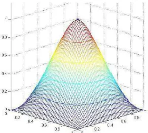
grows, the energy decreases (as explained earlier), and we stop the iteration when the decrease is less than a treshold. Figure 1 shows the resulting surface, within a treshold of 104. Note that u is like „one and a half‟ times

differentiable almost everywhere on

S

, so that the surface zu x y( , ) is not that smooth at (0.5, 0.5,1) .

Figure 1 The surface passing through (0.5,0.5,1) with minimum E_1.5( )u _.

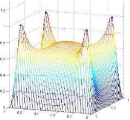
Figures 2-5 are obtained for different order  and/or different points

) , ,

(11)

are not that smooth at the prescribed points. The symmetry follows from the fact the prescribed points are of the same height and distributed evenly on

S

. It is interesting to observe that as the four points spread away, the surface shows four peaks. This relates to the fact that the solution is a linear combination of four functions whose graphs look like that in Figure 1 (but with different locations of the peak).

Figure 2 The surface passing through (0.5,0.5,1) with minimum curvature.

(12)

Figure 4 A surface passing through four prescribed points with minimum 1.5( )

E u _.

Figure 5 Another surface passing through four prescribed points with minimum )

(

1.5 u

E

.

4 The Case

01

(13)

uniqueness of such a function is guaranteed by Theorem 2.5, but as we shall see now the continuity is lost.

Recall that if

v

:=

[

a

_mn

]

is an element of

V

, then , =1

sin 0.5 sin 0.5 = 0.

mn m n

a m n





This implies that the only element that is orthogonal to

V

is 2 2

sin 0.5 sin 0.5 :=

( )

m n

u

m n 

 

 

 _ 

  or its multiples. But then we have

2 2 1 2 2 2

2 1 ...

5 9 13 17 25 1 1

2 1 3. 5. ... 9 25 .

u  _ _ _ _ _

      _       _      _    _    

Thus V={0} or V =W, the whole space. This tells us that, starting from any initial approximation

u

₀, we will end up with u=u₀proj ( ) = 0_V u₀ , that is,

0 = ) , (x y

u almost everywhere on

S

. Since we wish to keep the value 1 at

(0.5,0.5), the function u cannot be continuous on

S

. For instance, if we start from

u

0

(

x

,

y

)

=

sin



x

sin



y

, then we will end up with







.

0,

(0.5,0.5),

=

)

,

(

1,

=

)

,

(

therwise

o

y

x

y

x

u

This result is actually predictable in the case =0, that is, when we minimize the volume under the surface z=u(x,y), subject to the condition

0 = ,1) ( = ,0) ( = ) (1, = )

(0,y u y u x u x

u and u(0.5,0.5)=1.

To sum up, to have a continuous solution to our minimization problem, the condition >1 is not only sufficient but also necessary.

Acknowledgement

(14)

having translated our ideas into the codes. The authors also thank the referees for their useful comments on the earlier version of the paper.

References

[1] Alghofari, A.R., Problems in Analysis Related to Satellites, Ph.D. Thesis, The University of New South Wales, Sydney, 2005.

[2] Langhaar, H.L., Energy Methods in Applied Mechanics, John Wiley & Sons, New York, 1962.

[3] Gunawan, H., Pranolo, F. & Rusyaman, E., An Interpolation Method that

Minimizes an Energy Integral of Fractional Order, in D. Kapur (ed.), ASCM 2007, LNAI 5081, Springer-Verlag, 2008.

[4] Wallner, J., Existence of Set-Interpolating and Energy-Minimizing

Curves, Comput. Aided Geom. Design, 21, 883-892, 2004.

[5] Wan, W.L., Chan, T.F. & Smith, B., An Energy-Minimizing Interpolation

for Robust Multigrid Methods, SIAM J. Sci. Comput. 21, 1632-1649,

1999/2000.

[6] Ardon, R., Cohen, L.D. & Yezzi, A., Fast Surface Segmentation Guided

by User Input Using Implicit Extension of Minimal Paths, J. Math.

Imaging Vision, 25, 289-305, 2006.

[7] Benmansour, F. & Cohen, L.D., Fast Object Segmentation by Growing

Minimal Paths from A Single Point on 2D or 3D images, J. Math.

Imaging Vision, 33, 209-221, 2009.

[8] Capovilla, R. & Guven, J., Stresses in Lipid Membranes, arXiv: cond-mat/0203148v3, 2002.

[9] Stein, E.M., Singular Integrals and Differentiability Properties of

Functions, Princeton University Press, Princeton, 1971.

[10] Rao, C.R. & Rao, M.B., Matrix Algebra and Its Applications to Statistics

and Econometric, World Scientific, Singapore, 1998.

[11] Lorentz, G.G., Approximation of Functions, AMS Chelsea Publishing, Providence, 1966.

[12] Atkinson, K. & Han, W., Theoretical Numerical Analysis: A Functional