Is child labor harmful? the impact of working as a child on adult earnings

(1)

Is Child Labor Harmful?

The Impact of Working as a Child on Adult Earnings

Patrick M. Emerson

Department of Economics University of Colorado at Denver

patrick.emerson@cudenver.edu

André Portela Souza

Department of Economics University of São Paulo

&

Vanderbilt University aps@usp.br

November 2004

Abstract

This paper explores the question: is working as young laborer harmful to an individual in terms of adult outcomes in income? This question is explored through the utilization of a unique set of instruments that control for the decision to work as a child and the decision of how much schooling to acquire. These instruments are combined with two large household survey data sets from Brazil that include retrospective information on the child labor and schooling of working-age adults: the 1988 and 1996 PNAD.

Estimations of the reduced form earnings model are performed first by using OLS without controlling for the potential endogeneity of child labor and schooling, and then by using a GMM estimation of

instrumental variables models that include the set of instruments for child labor and schooling. The findings of the empirical investigations show that child labor has large negative impact on adult earnings for both male and female children even when controlling for schooling. In addition, the negative impact of starting to work as a child reverses at around age 14. Finally, different child labor activities are examined to determine if some are beneficial while others harmful with the finding that working in agriculture as a child appears to have no negative impact over and above the loss of education.

(JEL classification numbers: J31, O12, O54)

(Keywords: Child Labor, Brazil, Cost of Child Labor)

Acknowledgements: For useful comments and advice, we thank Christopher Dunn, Eric Edmonds, Ken Swinnerton and Tracy Regan. This paper has also benefited from seminar presentations at the 2004

(2)

Is Child Labor Harmful?

The Impact of Working as a Child on Adult Earnings

I. Introduction

Child labor is widespread in today’s world; the International Labour Organization

estimates that 246 million of the world’s children, or 16 percent, are child laborers, most

living in developing countries.1 Recently, there has been a renewed interest in child labor

issues, and this renewed interest has led to a series of studies that aim to understand the

causes and consequences of child labor in order to guide appropriate policy responses

(see Basu (1999), for a useful survey of the theoretical and empirical literature). Among

the policy options discussed are banning child labor and/or sanctioning countries that

allow the practice. These types of policy responses have been widely debated among

economists (see e.g., Emerson and Knabb, 2004; Basu, 2002; Dessy and Pallage, 2001;

Baland and Robinson, 2000; Dessy, 2000; Basu and Van, 1998). Most of these studies

emphasize the trade-off between child labor and human capital accumulation to justify

policy interventions, arguing that there are large negative consequences from child labor.

Child labor, however, is a catch-all term that encompasses a diversity of activities and

working conditions, thus the belief that child labor is detrimental to human capital

accumulation, may or may not be generally true, and, if so, at what age does this adverse

effect cease to exist, and does the initial occupation matter, are open questions.2

1

Child labor was also common in developed countries until fairly recently, see, e.g., Kruse and Mahony, 2000.

2

(3)

Studying and providing robust estimates of the effects of starting to work as a child on

adult earnings will allow future studies of child labor, and discussions of appropriate

policy responses, to be informed by these efforts.

Despite the fact that there is a large and growing literature on child labor, this one

fundamental question remains unanswered: does child labor harm participants? Though

it has been assumed to be detrimental, the potential effects of child labor on adult

earnings are twofold. On one hand, child labor can be detrimental through the hindering

of the acquisition of formal education, both quantitatively and qualitatively, and causing

irreparable damage to health, reputation or other things that effect adult human capital,

which could lead to lower wages in the adult labor market. On the other hand, there are

many reasons why one might expect that there can be positive pecuniary benefits to

young labor: vocational training, learning by doing, general workplace experience as well

as the potential for making contacts, learning job market strategies, etc. In other words,

there are many reasons to expect that a young laborer can gain some human capital from

their workplace experience (e.g., Horn, 1994). Thus the net effect of starting to work as a

child is an empirical issue. Though virtually all studies of child labor assume it is

harmful, there is as yet no reliable measure of the effects of working as a child on adult

outcomes.

These effects will also likely depend on the particular type of labor the child

undertakes because some jobs may lead to the acquisition of job specific human capital

while others may not. For example it could be that a child that works as manual laborer

in agriculture does not learn many skills that the adult labor market values. However, a

(4)

the blacksmith trade that are valuable on the adult labor market. For instance, French

(2002) finds that child workers in shoe manufacturing industries in Brazil have positive

attitudes toward their jobs if their work is associated with more autonomous and

self-directed tasks. Furthermore, child labor could be a way to finance education that an

individual would not otherwise have access to, which, in turn, could lead to better

outcomes for older child or adolescent workers (see, e.g., Akabayashi and

Psacharopoulos, 1999; Psacharopoulos, 1997).

Thus there is a startling gap between what is known about the causes of child

labor and what is known about the consequences of child labor.3 This paper seeks to fill

this gap by providing a detailed analysis of two large survey datasets that contain

retrospective information on the child labor of subjects and current information on their

incomes.

This study analyzes the effects of starting to work as a child on the adult earnings

of working age Brazilian men. Specifically, there are three main questions we will seek

to answer: One, what is the effect on adult earnings of starting to work as a child both

including the effect on educational attainment and the effect over and above the impact

on schooling? Two, when does the negative effect of working as a child (if there is one)

cease and positive effects commence? Third, are there differences in these effects

depending on which child labor occupations, or types of work, a child enters when first

starting to work?

3

(5)

There are two main reasons for the lack of prior studies of this type: the paucity of

good data and the confounding effects of potentially endogenous variables. The present

study is able to overcome both limitations.

The first limitation is particular to developing countries where data of a high

enough quality and a proper set of variables are hard to find. The Brazilian government,

however, has been a pioneer in the collection and dissemination of data and thus Brazil

presents a source of data that is adequate to address this complex relationship. The data

utilized in this paper come from two rounds of a very large household survey from Brazil

that includes information on current working-age adults’ attributes and incomes as well

as retrospective information on the age at which they first started to work and the number

of years they attended school. Importantly, these data sets also include information on

the educational attainment of the parents of the current working-age adults allowing

controls for the family background of the subject individuals to be controlled for. These

two data sets provide a very large and rich dataset from which to perform the analysis.

The second limitation is common to all studies that try and estimate the human

capital - earnings relationship, which can be traced back to the seminal research of

Becker and Chiswick (1966), Chiswick (1974) and Mincer (1974). Because of the strong

likelihood that there are unobserved attributes (e.g. ability) that effect both the schooling

choice of an individual and the individual’s adult earnings, estimates that do not attempt

to address this issue are considered unreliable. Recent research into this relationship

using US data has relied on the use of instrumental variables to overcome the

confounding effects of these unobserved attributes (Cameron and Taber, 2004; Carneiro

(6)

type of approach is that it demands a robust set of instruments for the schooling choice of

an individual. What makes this approach particularly challenging in the context of child

labor is that schooling and child labor are likely jointly determined, so a set of suitable

instruments must include instruments for both choices. To assemble a rich enough set of

instruments, data on the number of primary, secondary and college-level schools in each

Brazilian state for each year from 1933 to 1976 was collected, along with the number of

teachers per school in each state and year. These institutional variables are hypothesized

to be correlated with the work and schooling decisions of children (regardless of who

made these choices), yet uncorrelated with adult incomes (when netting out state and

other confounding effects). Statistical tests confirm the validity of these instruments.

With these two obstacles overcome, it is possible to provide a very detailed and

robust estimation of the effects of child labor on adult incomes both including the effect

of lost education and the effect over-and-above the effect on education. These results

should be of vital interest to researchers of child labor in their quest to understand both

the causes and consequences of child labor. This study then proceeds to test for

differences in these observed effects of starting to work as a child by the occupation

choice the person made when they first started to work.

The rest of this paper is organized as follows. Section 2 describes the data

utilized in this study. Section 3 discusses the empirical strategy employed to explore the

central questions of the paper. Section 4 presents the results of the empirical estimations.

(7)

II. The Data

The main sources of data utilized in this study are two rounds of the Pesquisa

Nacional por Amostragem a Domicílio (PNAD), from Instituto Brasileiro de Geografia e Estatística (IBGE), the Brazilian census bureau: 1988 and 1996. The PNAD is a yearly

and nationally representative household survey (excepting the rural Amazon region)

similar to the Current Population Survey in the U.S. It covers close to one hundred

thousand households and includes information on the demographic and labor market

characteristics of the households. Additionally, and of particular utility for the present

study, the 1988 and 1996 surveys obtain retrospective information from the household

head and the spouse about the age they entered the labor market, their first occupation,

the educational attainment of their parents as well as the occupation of their fathers when

they (head and spouse) first entered the labor market, the state in which they were born

and the state they currently reside in. If the two states were different, a follow-up

question was asked about the number of years the individual had lived in the current

state. This information was coded 1 through 10+ years.

Additional data on the number of primary schools, secondary schools and colleges

by state and year come from the IBGE Historical Series, 2003. Data on the number of

teachers per state per year were also collected from the IBGE. In order to match each

individual with the number of schools in their state for each year that they were school

aged (and later the number of teachers per school as well) we followed the following

procedure. If the individual was a current resident of the same state in which they were

born, we assume that they have not migrated and give them the number of schools

(8)

were current residents of and the migration information does not allow us to determine

exactly when they moved, we give them the national average number of schools for each

year they were of school age. Finally, if there is enough information to determine exactly

when migration occurred, we give the individual the appropriate instruments for the state

or states in which the resided during their school-aged years.

Our sample consists of all adult males who are between 25 and 55 years of age at

each survey year. We exclude younger and older men in an attempt to avoid potential

selectivity bias of labor participation decisions. We also exclude females for three

reasons: first, there is a large selection issue relating to the women who choose to work

(less than 50% of women in the 1988 and 1996 PNADs were listed as currently

employed); second, many girls work in the household rather than for wages leading to

under-measurement of female child labor; and third, fertility issues complicate the school

and work decisions of females. Because of these three concerns, females are excluded

from the current study though their outcomes are no less important. Hopefully future

research will be conducted that will focus on females. Unlike women, most of these

prime age male workers are likely to work in the labor market (over 95% work). We

perform all analyses on three samples: the 1988 and 1996 PNADs and a combined

sample of both in which we control for cohort effects. The combined sample consists of

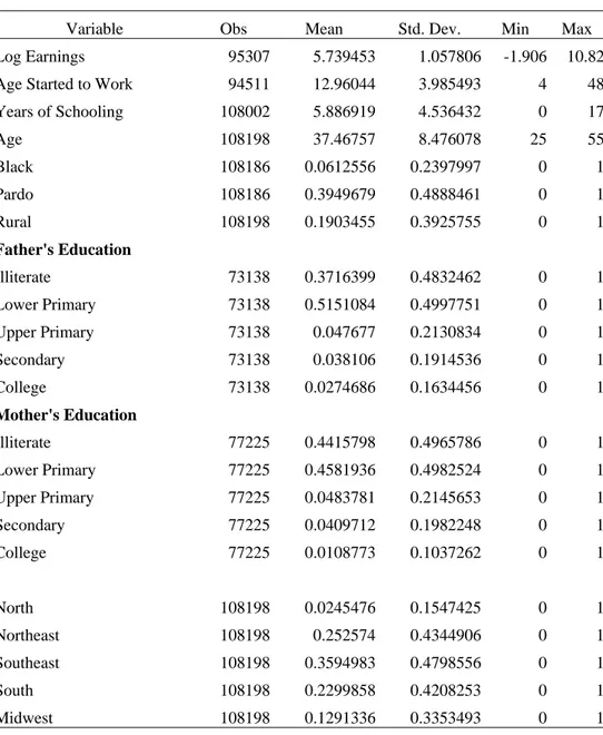
approximately 72,000 complete observations for men. The basic statistics of the

combined sample are presented in Table A1 of the Appendix.

Before discussing the regression analysis, it is informative to show the

distribution of the age started to work, the schooling attainment, and the log-earnings of

(9)

started to work for males. We divide the age started to work into four groups: those that

reported age started to work at nine years old or below, between ten and thirteen years

old, between fourteen and seventeen years old, and those at eighteen years old or above.

Around twenty percent of prime age male workers reported that they started to work at

nine years old or below for both surveys and around forty percent of them started to work

between ten and thirteen years old. Around twelve to fifteen percent of male workers

started to work at age eighteen or above.

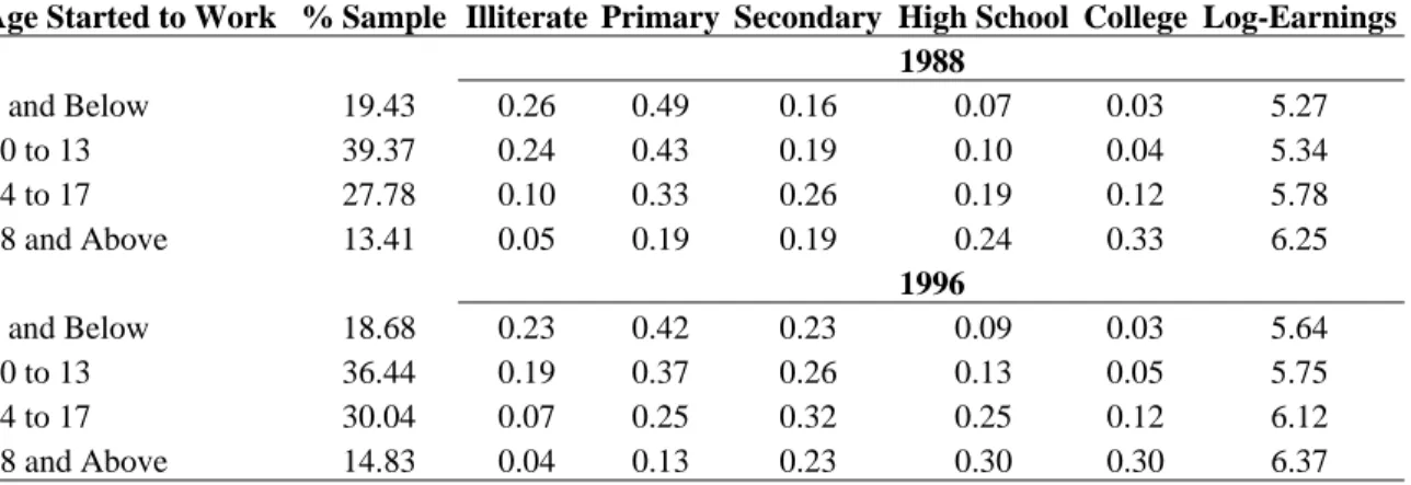
Table 1 also shows the distribution of schooling attainment and log-earnings by

each age-started-to-work group. We divide individuals into five educational attainment

groups: illiterates, some primary or completed primary education, some secondary or

completed secondary education, some high school or completed high school education,

and some college or completed college education. Table 1 reveals that individuals who

started to work earlier in life have lower educational attainments and lower earnings as

adults. For educational attainment, for instance, 26 percent of all prime-age males that

started to work at age nine or below are illiterate and two percent of them have some

college or completed college education in 1988. Conversely, five percent of all

prime-age males that started to work at eighteen years old or above are illiterates and 33 percent

of them have some college or completed education in 1988. Thus, Table 1 appears to

show that there is a direct relationship between the age and individual starts working and

their educational attainment and adult earnings. If a causal relationship between

age-started-to-work and adult earnings exists, its effect could be indirect (through education),

direct (through experience), or both. The next section presents the empirical strategy

(10)

III. Empirical Strategy

In the typical Micerian framework of the effect of schooling on adult earnings in

the high income country context, the discussion of the empirical issues usually begins

with a presentation of a standard two equation system that describes schooling (Si) and

log wages (lnYi), for an individual i:

(1) S_i = X_iδ+ν_i,

(2) lnYi =Xiγ+Siβ+υi.

In this case Xi is a vector of observed attributes of the individual and νi and υi are the

random error terms that are assumed to be uncorrelated with Xi. The coefficient β is a

measure of the ‘returns to education,’ or average returns to education if this varies across

individuals if ν_i and υ_i are uncorrelated.

It is quite likely that schooling is correlated with the unobserved component of the

log earnings equation, however, due to ability bias (see, e.g. Griliches (1977)),

measurement error in schooling, or a systematic variation in the returns to schooling

based on years of schooling (higher marginal returns in earlier years of schooling, see

Card (1995), for example).4 Ability bias arises when individuals of high ability both

acquire higher levels of schooling (because the returns are higher and/or the costs are

lower) and earn higher wages in the adult labor market. If this is true for our sample, an

estimation of the β coefficient will be biased upwards. Measurement error in schooling

can also bias the results if it induces a negative correlation between the errors of the

4

(11)

observed schooling and earnings, which would bias the estimate of β downward.

Finally, if individuals with lower levels of schooling have systematically higher returns to

schooling (due to diminishing marginal returns to schooling in general) then estimates of

β will also be downward biased.

The context of a low income country in which child labor is widespread presents

another confounding effect: child labor itself. The decision to work as a child is likely

correlated with the schooling decision and is also likely correlated with adult earnings.

Fortunately, one aspect of child labor is observed: the age at which individuals first

started to work. Therefore, in the low income country context, where child labor is

widespread the schooling and child labor decision are both likely to effect adult returns to

education and are likely correlated, a description of this process would involve a three

equation system for and individual i:

(1) Si = Xiδ+νi,

(2) CL_i = X_iα+ψ_i,

(3) lnY_i =X_iγ+S_iβ+CL_iφ+υ_i.

Where CLi is the age at which the individual first started to work, and ψi is the

unobserved random error term. In order for φ to be a measure of the effect of starting to

work at a certain age (or average if it varies across individuals), ψ_i and υ_i must be uncorrelated.

These error terms are likely correlated because of the same ability bias that causes

high ability individuals to choose more schooling may cause those individuals to choose

to start to work at an older age (biasing the coefficient estimate upward) or they may

(12)

market as well as the adult labor market (biasing the coefficient estimate downward).

Measurement error is another source of potential bias.

In this case, consistent estimates for the return to education and the effect of

starting to work as a child can be obtained if there is a set of regressors, Zi, that can be

added to the vector Xi that affect schooling but do not affect the unexplained component

of earnings, and that affect the age an individual starts to work but not the unexplained

component of earnings. This set of regressors must be sufficiently correlated with both

schooling and the age started to work (i.e. have enough separate correlation with both

variables that is separate from the correlation among the two variables), and sufficiently

uncorrelated with the unexplained variation in adult earnings that they can be legitimately

excluded from the earnings equation.

One set of variables that may fulfill this requirement are the number of primary

schools, secondary schools and colleges per capita in the individual’s state in the year

that they are of the appropriate age to attend these schools. The presence of more schools

in the same state as the individual lowers the cost of attending school as travel costs are

reduced and students are more likely to be able to live at home and attend school. Lower

cost of education should increase investments in education, and cause delay in starting to

work. These are the instruments employed in the first set of regressions. Because schools

vary in size, the number of schools may not be adequate. For this reason the number of

teacher per school for each state and year are also employed in later estimations.

If these variables are proxying for other things that affect adult earnings that are

unexplained by the covariates in the earnings equation, like school quality for instance or

(13)

adequate instruments for the schooling choice and age at which the individual started to

work. It is important to note, however, that the education of the mother and father are

included as controls in the earnings equations. As parental education is, in general, a

very good proxy for family income and wealth, they are likely to be strong correlates of

school quality, local labor market conditions, etc.5

To test the model presented above, we estimate a series of OLS regressions and a

series of GMM IV regressions in order to capture the effect of being an adolescent

laborer on adult earnings. The first set of regressions will estimate the direct impact of

being a young laborer on adult earnings. The second set of regressions will identify the

first job occupations that are associated with higher or lower earnings conditional on

having been an adolescent laborer. The third set of regressions will add the effect of

having the same first job occupation and the father’s occupation.

IV Estimation and Results

4.1 The Effect of Starting to Work as a Child

In order to estimate the effect of having been a child worker on current adult

earnings, we start by estimating two separate earnings equations that include the age the

individual first started to work variable and its square, the age of the individual and its

square, indicator variables that equal one if the individual is classified as black and

another if the individual is classified as ‘pardo,’ or mixed race. Included in all

estimations are measures of the father’s and mother’s education levels. For both, these

are indicators for each level of education completed: lower primary, upper primary,

5

(14)

secondary and college. For these estimations, an indicator variable that equals one if the

individual resides in a rural area is included, as well as indicators for the regions of Brazil

the individual currently resides in. The difference in the two separate earnings equations

is that in the first estimations the years of schooling of the individual are not included and

in the second set, the years of schooling are included.

We begin by estimating the earnings model for the two survey years separately

and estimate each first by OLS and then using the set of instruments described above in a

GMM IV framework (excluding, for the moment, the number of teachers per school).

The first set of regressions does not control for the individual’s educational attainment.

The fact that an individual worked during childhood or adolescence will likely mean that

individual will have attained less education than a similar individual that did not work.

So, as a first step, the coefficients of the young labor indicator variables when not

controlling for education capture the expected forgone adult earnings of a young worker.

Table 2 presents the results for the 1988 sample. The first and fifth columns of

each table show the coefficient estimates of the OLS and the second-stage of the IV

regressions, respectively, when the individual’s schooling variables are not included.6

First, as we are interested in the young laborer status of the individual and its impact on

his adult earnings, the coefficient estimates show that the older the individual enters the

labor market, the higher are his earnings (including the effect of the loss of education).

For the IV estimation, the squared term is negative and significant, suggesting that this

negative effect ceases at around age 14. Thus, there is a negative and significant impact

on adult earnings if a male individual started to work as a child at or below the age of 14,

(15)

The third and seventh columns of Table 2 present the coefficient estimates of the

OLS and second-stage IV regressions, respectively, when the individual’s schooling

variables are included. Thus the coefficients estimates of the young laborer indicator

variables reflect the effect on adult income of having been a young laborer

over-and-above the loss of education. Here, the age started to work coefficient estimate is still

positive for both and its square is positive again for the IV estimation.

For all four estimations, the other coefficient estimates have the expected signs.

Older individuals have higher earnings but this increases at a decreasing rate, black and

pardo individuals have systematically lower earnings than white individuals, individuals

in rural areas have lower earnings, and, the more educated the parents are, the greater the

earnings of the individuals.

Table 3 presents the same estimations for the 1996 survey year with qualitatively

the same results. The IV estimates are again above the OLS estimates for the return to

schooling and the negative effect of starting to work holding schooling constant ceases

around age 15.

Table 4 presents the estimates for these same models for a pooled sample that

includes an indicator for the 1988 survey year and indicators for cohorts: one for

individuals born in the years 1933 to 1945, and another for individuals born in

1946-1958. The pooled sample estimations follow the same pattern of results as the preceding

estimations. The ’46-’58 cohort indicator variable estimate is positive and significant in

all cases and, interestingly, individuals from the earlier sample, 1988, have systematically

lower earnings, perhaps reflecting the growth of the Brazilian economy over the

intervening years.

6

(16)

Together, these results suggest that there is indeed a negative impact of being a

child labor both including the effect on educational attainment and over and above the

impact on education. However, this effect seems to subside and turn positive at around

age 13-14. Figure 1 presents an ‘iso-earnings’ curve the represents the trade-off between

education and child labor based on the estimated coefficients from Table 4. While the

magnitude of the impacts may be imprecisely estimated for reasons stated above, there

seems to be no reason, a priori, that the turning point of the effect of child labor on adult

earnings to be biased. From these exercises the picture that emerges is that though there

is an important impact of adolescent labor on adult earnings through the trade-off with

schooling, there is a strong impact over and above the effect on educational attainment

and that this impact turns positive around age 13-14.

Like similar studies of the education – earnings relationship in the United States

and elsewhere, the IV regression coefficient estimates on the schooling variable are

systematically higher than the OLS coefficient estimates. This may seem

counter-intuitive if one believes that we are correcting for ability bias, something that should bias

the OLS estimates upward. However, as Griliches (1977) and others have pointed out,

measurement error in the schooling variable can lead to a downward attenuation bias in

the OLS estimate, something that IV, as long as the instruments are not correlated with

the measurement error, corrects for. In addition, as Card (1999) points out, if the

individuals for whom school location is most important in determining their education

(perhaps due to credit constraints) are also the ones who have the highest marginal impact

from schooling, then school location as an instrument will emphasize their contribution to

(17)

developing countries, this may explain the higher estimates of the return to schooling

than those from the US and other developed countries.

Table 5 presents OLS and IV estimates using the 1996 sample but with the

number of teachers per school for each state and year included as additional instruments

for the child labor and schooling decisions. In order to use a more parsimonious set of

instruments we have restricted the number of schools and number of teachers per school

to just the ages 7 through 12. The results of this estimation are given in Table 5.

Compared to the 1996 results without the teacher instruments the coefficient estimates on

the age started to work variables, and the schooling variable, have increased. The turning

point for the iso-earnings curve is at age 13.1, relatively consistent with the previous

results.

4.2 The Role of Different Child Labor Activities

Since some activities that children may engage in when they work may have good

vocational or other job training aspects to them, we next attempt to identify any particular

activities that appear to have positive human capital. The distribution of first job

occupations for the pooled sample is given in Table 6. We construct five occupational

categories from the three-digit occupation categories available in PNAD.7 These

categories are somewhat arbitrary at the margins since there do not exist very clear

boundaries between the many occupations, but for the most part, capture the occupations

generally associated with these activities. As Table 6 shows, the bulk of male child labor

was devoted to agricultural activities. Between the two survey years there is a decrease

in the percentage of child laborers in agriculture and an increase in the percentage of

7

(18)

child laborers in civil construction and manufacturing. This trend may reflect the

increase in the urbanization in Brazil during that time period.

In order to estimate the impact of these specific child labor occupations on adult

earnings, we estimate a series of IV models, similar to those presented previously that

included schooling, but for each first job occupation separately. Also included are an

indicator variable that equals one if the first job occupation of the individual was the

same as the fathers occupation, and an interaction of this variable with age started to

work. The coefficient estimates from these estimations are presented in Table 7. The

key results here are that the effect of age started to work are similar to those not separated

by occupation for commerce and transport and for services and others: positive and

significant coefficient estimates for age started to work and negative and significant

estimates for its square. Significant estimates are not obtained for the other three

categories. This is not surprising for manufacturing and civil construction as they

represent less than 10 percent and 5 percent of the sample, respectively. However the

fact that the sign of the point estimate for the age started to work variable for the

agricultural regression is negative, and the fact that agriculture accounts for almost 40%

of the sample is intriguing. This suggests that there may be no adverse effect from

starting to work as a child, over and above the impact on schooling, for those that

undertake agricultural activities. This is a particularly important result when one

considers the fact that worldwide, 70 percent of child workers are estimated by the ILO to

work in agriculture and related activities.

Thus there appears to be evidence that in some occupations entering as a child

(19)

V. Conclusion

In this paper, we investigated the effect of starting to work as a child laborer on an

individual’s adult earnings. We find that child labor is associated with lower adult

earnings, partly due to the trade-off associated with educational attainment and partly due

to the effect over and above the impact on educational attainment, but that this negative

effect appears to reverse in the age rage of 13-15.

Second, although there appears to be some decrease in adult earnings in general

from child work beyond schooling, we find that for agricultural activities there appears to

be no adverse effect. Particularly important for females is domestic work, which does not

seem to harm the adolescent worker. Finally, we find that there are no gains for male

(20)

REFERENCES

Akabayashi, Hideo and George Psacharopolous. (1999) “The Trade-off Between Child

Labor and Human Capital Formation: A Tanzanian Case Study,” Journal of

Development Studies, v. 35, June.

Baland, Jean-Marie, and James A. Robinson. (2000) “Is Child Labor Inefficient?,”

Journal of Political Economy, v. 108, n. 4.

Basu, Kaushik. (2002) “A Note on Multiple General Equilibria with Child Labor,”

Economics Letters, v. 74, n. 3.

Basu, Kaushik. (1999) “Child Labor: Cause, Consequence, and Cure,” Journal of

Economic Literature, v. 37, n. 3.

Basu, Kaushik and Pham Hoang Van. (1998) “The Economics of Child Labor,”

American Economic Review, v. 88, n. 3.

Cameron, Stephen V., and Christopher Taber. (2004) “Estimation of Educational

Borrowing Constraints Using Returns to Schooling,” Journal of Political

Economy, Vol. 112, no. 1, pt. 1, pp. 132-182.

Card, David. (2001) “Estimating the Returns to Schooling: Progress on Some Persistent

Econometric Problems,” Econometrica, Vol. 69, pp. 1127-1160.

__________. (1999) “The Causal Effect of Education on Earnings.” The Handbook of

Labor Economics, Orley Ashenfelter and David Card, eds. (New York: Elsevier).

__________. (1995a) “Earnings, Schooling and Ability Revisited,” Research in Labor

Economics, Vol. 14, n. 1, pp. 23-48.

__________. (1995b) “Using Geographic Variation in College Proximity to Estimate the

Return to Schooling.” Aspects of Labour Market Behavior: Essays in Honor of

John Vanderkamp, Louis N. Christofides, E. Kenneth Grant, and Robert

Swidinsky, eds. (Toronto: University of Toronto Press).

Carneiro, Pedro, and James J. Heckman. (2002) “The Evidence on Credit Constraints in

Post-Secondary Schooling,” The Economic Journal, Vol. 112, pp. 705-734.

Chiswick, Barry R. (1974) Income Inequality: Regional Analyses Within a Human

(21)

Chiswick, Barry R., and Jacob Mincer. (1972) “Time Series Changes in Personal Income

Inequality,” Journal of Political Economy, Vol. 80, n. 3, Part 2, pp. S34-S66.

Dessy, Sylvain. (2000) “A Defense of Compulsive Measures against Child Labor,”

Jounal of Development Economics, v. 62, n.1.

Dessy, Sylvain and Stephane Pallage. (2001) “Child Labor and Coordination Failures,”

Journal of Development Economics, v. 65, n. 2.

Duryea, Suzanne. (1998) “Children’s Advancement Through School in Brazil: The Role

of Transitory Shocks to Household Income,” Inter-American Development Bank

Working Paper 376.

Emerson, Patrick M., and Shawn D. Knabb. (2004) “Expectation Traps, Intergenerational

Redistribution and Child Labor,” Mimeo, University of Colorado at Denver.

Emerson, Patrick M., and André Portela Souza. (2003) “Is there a Child Labor Trap?

Inter-Generational Persistence of Child Labor in Brazil,” Economic Development

and Cultural Change, 51:2, pp. 375 - 398.

French, J. Lawrence. (2002) “Adolescent Workers in Third World Export Industries:

Attitudes of Young Brazilian Shoemakers,” Industrial and Labor Relations

Review, Vol. 55, n. 2, January.

Gangadharan, Lata, and Pushkar Maitra. (2001) “Two Aspects of Fertility Behavior in

South Africa,” Economic Development and Cultural Change, Vol. 50, n. 1, pp.

183-200.

Griliches, Zvi. (1977) “Estimating the Returns to Schooling: Some Econometric

Problems,” Econometrica, Vol 45, n. 1, pp. 1-22.

Horn, Pamela. (1994) Children’s Work and Welfare, 1780-1890. (Cambridge:

Cambridge University Press).

Ilahim, Nadeem, Peter Orazem and Guilherme Sedlacek. (2000) “The Implications of

Child Labor for Adult Wages, Income and Poverty: Retrospective Evidence from

Brazil,” mimeo.

Keane, Michael P., and Kenneth I. Wolpin (2001) “The Effect of Parental Transfers and

Borrowing Constraints on Educational Attainment,” International Economic

(22)

Klawon, Emily, and Jill Tiefenthaler (2001) “Bargaining over Family Size: The

Determinants of Fertility in Brazil,” Population Research and Policy Review, Vol.

20, n. 5, pp. 423-40.

Kruse, Douglas L. and Douglas Mahony. (2000) “Illegal Child Labor in the United

States: Prevalence and Characteristics,” Industrial and Labor Relations Review, v.

54, n. 1.

Lam, David. (1986) “The Dynamics of Population Growth, Differential Fertility, and

Inequality,” American Economic Review, Vol. 76, n. 5, pp. 1103-1116.

Lam, David and Suzanne Duryea. (1999) “Effects of Schooling on Fertility, Labor

Supply, and Investments in Children, With Evidence from Brazil,” Journal of

Human Resources, Vol. 34, n. 1, pp. 160-92.

Mincer, Jacob. (1974) Schooling, Experience and Earnings. (New York: Columbia

University Press for NBER).

Neri, M., Emily Gustafsson-Wright, Guilherme Sedlacek, Daniela Ribeiro da Costa &

Alexandre Pinto (2000) “Microeconomic Instability and Children's Human

Capital Accumulation: The Effects of Idiosyncratic Shocks to Father's Income on

Child Labor, School Drop-Outs and Repetition Rates in Brazil,” Ensaios

Econômicos, EPGE, 394, Getulio Vargas Foundation, Brazil

Parsons, Donald O. and Claudia Goldin. (1989) “Parental Altruism and Self-Interest:

Child Labor Among Late Nineteenth-Century American Families”, Economic

Inquiry, v. 28, October.

Psacharopolous, George (1997), “Child Labor versus Educational Attainment: Some

Evidence from Latin America”, Journal of Population Economics, v. 10, October.

Spindel, Cheywa R. (1985) O Menor Trabalhador: Um Assalariado Registrado. São

(23)

Table 1: Schooling Distribution and Mean Log-Earnings by Age Started to Work 25 to 55 Year-Old Males

Age Started to Work % Sample Illiterate Primary Secondary High School College Log-Earnings 1988

9 and Below 19.43 0.26 0.49 0.16 0.07 0.03 5.27

10 to 13 39.37 0.24 0.43 0.19 0.10 0.04 5.34

14 to 17 27.78 0.10 0.33 0.26 0.19 0.12 5.78

18 and Above 13.41 0.05 0.19 0.19 0.24 0.33 6.25

1996

9 and Below 18.68 0.23 0.42 0.23 0.09 0.03 5.64

10 to 13 36.44 0.19 0.37 0.26 0.13 0.05 5.75

14 to 17 30.04 0.07 0.25 0.32 0.25 0.12 6.12

(24)

Table 2:

Dependent Variables

Coeff. Std. Error Coeff. Std. Error Coeff. Std. Error Coeff. Std. Error

Age Started to Work 0.033 *** 0.009 0.021 *** 0.006 1.495 *** 0.334 1.460 *** 0.322

Age Started to Work Squared 0.000 0.000 0.000 * 0.000 -0.045 *** 0.012 -0.050 *** 0.011

Years of Scholing 0.112 *** 0.002 0.205 ** 0.082

Age 0.115 *** 0.010 0.102 *** 0.008 0.152 *** 0.020 0.131 *** 0.020

Age Squared -0.001 *** 0.000 -0.001 *** 0.000 -0.002 *** 0.000 -0.001 *** 0.000

Back -0.390 *** 0.022 -0.246 *** 0.020 -0.489 *** 0.046 -0.236 ** 0.118

Pardo -0.290 *** 0.013 -0.189 *** 0.012 -0.346 *** 0.031 -0.185 ** 0.075

Father's Education

Lower Primary 0.233 *** 0.012 0.062 *** 0.011 0.053 0.062 -0.188 0.098

Upper Primary 0.535 *** 0.033 0.155 *** 0.030 0.129 0.169 -0.333 0.216

Secondary 0.673 *** 0.033 0.192 *** 0.031 0.304 0.251 -0.228 0.294

College 0.767 *** 0.042 0.255 *** 0.041 0.507 0.381 0.069 0.375

Mother's Education

Lower Primary 0.309 *** 0.012 0.116 *** 0.011 0.078 0.077 -0.160 0.107

Upper Primary 0.595 *** 0.034 0.219 *** 0.031 0.341 * 0.200 -0.075 0.238

Secondary 0.744 *** 0.034 0.320 *** 0.032 0.466 ** 0.236 -0.010 0.273

College 0.796 *** 0.057 0.381 *** 0.055 0.603 ** 0.290 0.220 0.307

Rural -0.629 *** 0.014 -0.399 *** 0.014 -0.316 *** 0.123 -0.065 0.129

North -0.225 *** 0.028 -0.162 *** 0.025 -0.312 *** 0.086 -0.124 0.111

Northeast -0.300 *** 0.022 -0.213 *** 0.018 -0.301 *** 0.043 -0.121 0.085

South -0.075 *** 0.026 -0.049 ** 0.022 -0.045 0.035 -0.040 0.029

Center-West -0.019 0.025 -0.032 0.020 0.181 *** 0.060 0.082 0.064

Constant 2.896 *** 0.193 2.744 *** 0.162 -8.434 *** 2.507 -7.917 *** 2.394

# Obs. 32,650 32,641 32,142 32,133

R-Squared 0.366 0.481

Hansen's J-Statistics 20.960 19.982

Chi-Squared (P-value) 0.074 0.067

Note: (1) *** statistically significant at 1%;** statistically significant at 5%;* statistically significant at 10%. (2) The instruments are the nubmer of school by state and year.

IV 3 IV 4

OLS and IV Estimates of Log-Earnings: 25-55 Year-Old Males 1988

(25)

Table 3:

Age Started to Work 0.034 *** 0.007 0.021 *** 0.006 1.349 ** 0.574 1.327 ** 0.538

Age Started to Work Squared 0.000 0.000 -0.001 *** 0.000 -0.041 * 0.023 -0.042 ** 0.021

Years of Scholing 0.105 *** 0.001 0.096 0.084

Age 0.105 *** 0.010 0.076 *** 0.008 0.123 *** 0.019 0.099 *** 0.030

Age Squared -0.001 *** 0.000 -0.001 *** 0.000 -0.001 *** 0.000 -0.001 ** 0.000

Back -0.383 *** 0.020 -0.257 *** 0.018 -0.469 *** 0.050 -0.352 *** 0.118

Pardo -0.311 *** 0.012 -0.211 *** 0.010 -0.324 *** 0.046 -0.239 *** 0.091

Lower Primary 0.250 *** 0.012 0.078 *** 0.011 0.059 0.064 -0.068 0.134

Upper Primary 0.409 *** 0.023 0.096 *** 0.020 0.020 0.238 -0.187 0.304

Secondary 0.593 *** 0.029 0.199 *** 0.028 0.154 0.316 -0.101 0.392

College 0.858 *** 0.035 0.404 *** 0.031 0.595 0.623 0.332 0.647

Lower Primary 0.240 *** 0.011 0.081 *** 0.010 0.062 0.062 -0.060 0.125

Upper Primary 0.472 *** 0.024 0.169 *** 0.023 0.220 0.174 -0.006 0.270

Secondary 0.640 *** 0.030 0.259 *** 0.027 0.396 0.312 0.130 0.397

College 0.648 *** 0.044 0.229 *** 0.041 0.393 0.302 0.095 0.410

Rural -0.619 *** 0.014 -0.407 *** 0.013 -0.206 * 0.119 -0.068 0.169

North -0.209 *** 0.033 -0.141 *** 0.029 -0.220 *** 0.077 -0.146 0.092

Northeast -0.298 *** 0.021 -0.212 *** 0.017 -0.273 *** 0.082 -0.182 * 0.101

South -0.057 ** 0.025 -0.025 0.020 0.046 0.058 0.059 0.055

Center-West -0.030 0.025 -0.035 0.021 0.169 *** 0.049 0.145 *** 0.049

Constant 3.381 *** 0.191 3.595 *** 0.159 -6.610 * 3.666 -6.198 * 3.490

# Obs. 31,725 31,646 31,495 31,416

R-Squared 0.376 0.489

IV 3 IV 4

IV Estimates of Log-Earnings: 25-55 Year-Old Males 1996

(26)

Table 4:

Age Started to Work 0.032 *** 0.006 0.020 *** 0.004 1.937 *** 0.415 2.248 *** 0.411 Age Started to Work Squared 0.000 0.000 0.000 *** 0.000 -0.066 *** 0.017 -0.083 *** 0.018

Years of Scholing 0.109 *** 0.001 0.165 ** 0.079

Age 0.085 *** 0.007 0.073 *** 0.006 0.115 *** 0.015 0.108 *** 0.017

Age Squared -0.001 *** 0.000 -0.001 *** 0.000 -0.001 *** 0.000 -0.001 *** 0.000

Back -0.386 *** 0.015 -0.251 *** 0.013 -0.509 *** 0.041 -0.327 *** 0.103

Pardo -0.301 *** 0.010 -0.200 *** 0.008 -0.383 *** 0.038 -0.277 *** 0.065

Lower Primary 0.240 *** 0.009 0.069 *** 0.008 0.113 * 0.061 -0.059 0.091

Upper Primary 0.449 *** 0.019 0.110 *** 0.016 0.305 0.204 0.094 0.201

Secondary 0.624 *** 0.022 0.191 *** 0.022 0.588 ** 0.292 0.384 0.278

College 0.815 *** 0.028 0.333 *** 0.026 1.255 ** 0.515 1.286 *** 0.481

Lower Primary 0.276 *** 0.008 0.099 *** 0.008 0.151 ** 0.067 -0.012 0.091

Upper Primary 0.519 *** 0.020 0.187 *** 0.019 0.504 *** 0.189 0.286 0.199

Secondary 0.689 *** 0.023 0.286 *** 0.021 0.819 *** 0.279 0.619 ** 0.272

College 0.708 *** 0.034 0.288 *** 0.032 0.881 *** 0.306 0.698 ** 0.309

Rural -0.627 *** 0.011 -0.404 *** 0.010 -0.406 *** 0.124 -0.261 ** 0.120

Cohort 1933-45 0.005 0.055 0.044 0.044 -0.062 0.071 -0.015 0.072

Cohort 1946-58 0.071 ** 0.032 0.063 ** 0.025 0.080 ** 0.039 0.076 ** 0.037

Year 1988 -0.366 *** 0.017 -0.315 *** 0.014 -0.324 *** 0.033 -0.212 *** 0.060

North -0.215 *** 0.023 -0.150 *** 0.021 -0.177 ** 0.083 0.021 0.130

Northeast -0.300 *** 0.019 -0.213 *** 0.015 -0.229 *** 0.057 -0.033 0.112

South -0.066 *** 0.022 -0.036 * 0.019 -0.053 0.044 -0.071 * 0.042

Center-West -0.025 0.020 -0.033 ** 0.016 0.135 *** 0.047 0.058 0.061

Constant 3.771 *** 0.147 3.632 *** 0.122 -9.666 *** 2.652 -11.402 *** 2.583

# Obs. 64,375 64,287 63,637 63,549

R-Squared 0.395 0.505

IV 3 IV 4

OLS and IV Estimates of Log-Earnings: 25-55 Year-Old Males Pooled 1988 and 1996

(27)

Table 5:

Coeff. Std. Error Coeff. Std. Error

Age Started to Work 2.155 *** 0.559 1.673 *** 0.486 Age Started to Work Squared -0.079 *** 0.022 -0.064 *** 0.019 Years of Scholing 0.192 ** 0.091 Age 0.147 *** 0.021 0.086 *** 0.033 Age Squared -0.002 *** 0.000 -0.001 * 0.000 Back -0.520 *** 0.071 -0.254 * 0.139 Pardo -0.414 *** 0.047 -0.218 ** 0.099

Lower Primary 0.214 *** 0.054 -0.064 0.140 Upper Primary 0.615 *** 0.204 0.078 0.302 Secondary 0.922 *** 0.274 0.237 0.387 College 2.009 *** 0.555 1.079 * 0.608

Lower Primary 0.194 *** 0.055 -0.059 0.125 Upper Primary 0.613 *** 0.167 0.098 0.272 Secondary 1.140 *** 0.293 0.419 0.403 College 1.057 *** 0.301 0.335 0.417

Rural -0.506 0.093 -0.204 0.159 North -0.011 0.121 0.053 0.102 Northeast -0.038 0.119 0.048 0.103 South 0.087 0.054 0.043 0.049 Center-West 0.164 *** 0.060 0.064 0.067 Constant -10.994 *** 3.626 -7.287 ** 3.287 # Obs. 31725 31646

R-Squared

Hansen's J-Statistics 8.64 7.95 Chi-Squared (P-value) 0.57 0.54

IV 3 IV 4

(28)

Table 6:

Distribution of First Job Occupation if Started to Work 14 Years Old or Below

First Job Occupation # OBS Percent

Agriculture 24,978 39.35

Manufacturing 5,910 9.31

Civil Construction 3,109 4.90

Commerce and Transport 6,416 10.11

Services and others 23,059 36.33

(29)

Table 7:

Coeff. Std. Error Coeff. Std. Error Coeff. Std. Error Coeff. Std. Error Coeff. Std. Error

Age Started to Work -2.142 2.319 0.830 0.666 0.775 0.495 0.937*** _0.298 _1.075** _0.428

Age Started to Work Squared 0.114 0.100 -0.023 0.026 -0.033 0.020 -0.033*** _0.012 _-0.036** _0.015

Years of Scholing 0.280 0.187 0.147** _0.066 _0.133 _0.091 _0.147*** _0.071 _-0.083 _0.130

Same Father's Occupation 6.775 5.227 -1.061 4.042 -2.260 4.888 -5.188* _3.009 _-4.575 _5.775

Interaction Age Sarted to Work

and Same Father's Occupation -0.321 0.471 0.084 0.378 -0.013 0.395 0.448**

0.209 0.440 0.462

Age 0.055 0.036 0.085*** _0.020 _0.122** _0.048 _0.067*** _0.029 _0.188*** _0.056

Age Squared 0.000 0.000 -0.001*** _0.000 _-0.001** _0.001 _-0.001 _0.000 _-0.002*** _0.001

Back -0.361 0.329 -0.346*** _0.072 _-0.193** _0.094 _-0.203 _0.138 _-0.651*** _0.249

Pardo -0.132 0.185 -0.131*** _0.044 _-0.211*** _0.064 _-0.095 _0.066 _-0.542*** _0.171

Lower Primary 0.000 0.203 -0.118 0.095 0.095 0.125 -0.122 0.127 0.405 0.292

Upper Primary -0.373 0.450 -0.255 0.157 0.170 0.297 -0.137 0.225 0.697 0.496

Secondary -1.167 0.907 -0.355 0.218 0.399 0.344 -0.079 0.308 0.971 0.598

College -2.457* _1.485 _-0.270 _0.331 _0.502 _0.806 _0.063 _0.401 _1.406** _0.698

Lower Primary -0.036 0.164 -0.047 0.083 -0.024 0.114 -0.035 0.124 0.408 0.277

Upper Primary -0.346 0.503 -0.085 0.175 0.200 0.372 0.013 0.225 0.877* _0.471

Secondary -0.375 0.709 -0.099 0.196 0.371 0.420 0.043 0.255 1.170** _0.574

College -0.344 1.373 -0.054 0.279 -0.006 0.683 0.045 0.284 1.206** _0.591

Rural 0.199 0.226 -0.035 0.142 -0.287** _0.129 _-0.006 _0.183 _-0.682* _0.366

Cohort 1933-45 0.062 0.131 0.008 0.113 0.003 0.212 0.081 0.118 -0.052 0.125

Cohort 1946-58 0.045 0.085 0.059 0.067 0.039 0.106 0.069 0.055 0.033 0.057

Year 1988 -0.362* _0.205 _-0.453*** _0.105 _-0.175 _0.185 _-0.246*** _0.055 _-0.013 _0.183

North 0.211 0.436 -0.118 0.206 0.120 0.181 -0.305*** _0.071 _-0.091 _0.127

Northeast 0.577** _0.264 _-0.198 _0.165 _-0.049 _0.116 _-0.176*** _0.067 _-0.201* _0.120

South 1.075** _0.448 _-0.116** _0.058 _-0.066 _0.108 _-0.013 _0.051 _-0.115** _0.048

Center-West 0.238* _0.128 _0.112 _0.092 _-0.217 _0.147 _0.042 _0.075 _0.147 _0.099

Constant 10.407 12.877 -3.163 4.342 -1.269 3.250 -2.585 2.179 -4.959 3.147

# Obs. 22,130 6,819 3,451 7,635 23,514

Hansen's J-Statistics 4.866 9.844 9.756 12.324 2.134

Chi-Squared (P-value) 0.900 0.454 0.462 0.264 0.995

Commerce and Transport Services and others IV Estimates of Log-Earnings: 25-55 Year-Old Males Pooled 1988 and 1996 - By First Job Occupation Categories

(30)

APPENDIX

Table A1: Summary Statistics for Pooled Sample 1988-1996 - Males Only

Variable Obs Mean Std. Dev. Min Max

Log Earnings 95307 5.739453 1.057806 -1.906 10.82

Age Started to Work 94511 12.96044 3.985493 4 48

Years of Schooling 108002 5.886919 4.536432 0 17

Age 108198 37.46757 8.476078 25 55

Black 108186 0.0612556 0.2397997 0 1

Pardo 108186 0.3949679 0.4888461 0 1

Rural 108198 0.1903455 0.3925755 0 1

Illiterate 73138 0.3716399 0.4832462 0 1

Lower Primary 73138 0.5151084 0.4997751 0 1

Upper Primary 73138 0.047677 0.2130834 0 1

Secondary 73138 0.038106 0.1914536 0 1

College 73138 0.0274686 0.1634456 0 1

Illiterate 77225 0.4415798 0.4965786 0 1

Lower Primary 77225 0.4581936 0.4982524 0 1

Upper Primary 77225 0.0483781 0.2145653 0 1

Secondary 77225 0.0409712 0.1982248 0 1

College 77225 0.0108773 0.1037262 0 1

North 108198 0.0245476 0.1547425 0 1

Northeast 108198 0.252574 0.4344906 0 1

Southeast 108198 0.3594983 0.4798556 0 1

South 108198 0.2299858 0.4208253 0 1

(31)

Table A2:

Coeff. Std. Error Coeff. Std. Error Coeff. Std. Error Coeff. Std. Error Coeff. Std. Error

Age 0.016 0.025 1.329 0.734 0.016 0.025 1.328 0.734 0.116 0.024 Age-Squared 0.000 0.000 -0.021 0.010 0.000 0.000 -0.021 0.010 -0.002 0.000 Back 0.073 0.096 -0.023 2.783 0.072 0.096 -0.035 2.783 -1.260 0.092 Pardo -0.104 0.048 -4.614 1.385 -0.105 0.048 -4.645 1.385 -0.916 0.046

Lower Primary 0.698 0.053 18.595 1.535 0.698 0.053 18.601 1.535 1.687 0.050 Upper Primary 1.949 0.133 53.710 3.883 1.949 0.133 53.710 3.883 3.855 0.128 Secondary 2.766 0.140 80.632 4.079 2.765 0.140 80.631 4.079 4.998 0.134 College 3.948 0.166 120.874 4.839 3.948 0.166 120.873 4.840 5.632 0.159

Lower Primary 0.884 0.051 23.626 1.499 0.884 0.051 23.628 1.499 1.933 0.049 Upper Primary 2.078 0.135 61.926 3.943 2.078 0.135 61.925 3.943 3.902 0.130 Secondary 2.528 0.139 75.432 4.053 2.528 0.139 75.429 4.054 4.520 0.133 College 2.773 0.249 85.620 7.250 2.773 0.249 85.617 7.251 4.483 0.238 Rural -1.432 0.051 -39.289 1.479 -1.431 0.051 -39.286 1.479 -2.381 0.049 North 0.892 0.095 25.110 2.775 0.893 0.095 25.162 2.776 -0.259 0.091 Northeast 0.412 0.057 11.454 1.673 0.413 0.057 11.488 1.674 -0.555 0.055 South 0.022 0.069 -0.810 2.001 0.023 0.069 -0.799 2.001 -0.053 0.066 Center-West -0.518 0.090 -13.185 2.611 -0.517 0.090 -13.169 2.612 0.025 0.086

Instruments

# of Schools at 6 -0.045 0.055 -1.386 1.600 -0.045 0.055 -1.384 1.600 -0.022 0.053 # of Schools at 7 0.112 0.120 1.943 3.488 0.111 0.120 1.937 3.488 0.185 0.115 # of Schools at 8 -0.265 0.170 -4.901 4.944 -0.265 0.170 -4.889 4.944 -0.438 0.163 # of Schools at 9 0.256 0.172 6.635 5.015 0.256 0.172 6.623 5.015 0.340 0.165 # of Schools at 10 -0.387 0.176 -11.905 5.137 -0.386 0.176 -11.887 5.138 -0.471 0.169 # of Schools at 11 0.154 0.171 3.762 4.984 0.154 0.171 3.756 4.984 0.478 0.164 # of Schools at 12 0.060 0.172 2.390 5.008 0.060 0.172 2.373 5.009 -0.175 0.165 # of Schools at 13 0.173 0.161 5.252 4.684 0.174 0.161 5.272 4.685 -0.073 0.154 # of Schools at 14 -0.166 0.149 -4.990 4.340 -0.167 0.149 -5.028 4.341 0.012 0.143 # of Schools at 15 0.042 0.147 -0.220 4.282 0.044 0.147 -0.185 4.283 0.167 0.141 # of Schools at 16 0.099 0.137 2.749 4.000 0.099 0.137 2.745 4.001 -0.130 0.132 # of Schools at 17 -0.029 0.124 1.484 3.611 -0.029 0.124 1.481 3.612 0.243 0.119 # of Schools at 18 -0.288 0.104 -7.398 3.034 -0.288 0.104 -7.395 3.035 -0.368 0.100 # of Schools at 19 0.659 0.244 19.842 7.096 0.658 0.244 19.801 7.097 0.610 0.233 # of School at 20 0.013 0.056 0.288 1.620 0.012 0.056 0.272 1.620 -0.041 0.053 Constant 11.276 0.635 112.561 18.499 11.280 0.635 112.679 18.501 2.660 0.608

Obs. 32142 32142 32133 32133 32133

Test of excluded Instruments

F( 15, OBS-K) 3.480 2.850 3.480 2.850 4.920

Prob > F 0.000 0.000 0.000 0.000 0.000

Partial R-squared of Excuded Instruments

0.002 0.001 0.002 0.001 0.002

Shea's Partial R-Squared

0.002 0.001 0.001 0.001 0.001

Age Started to Work 2 Schooling IV 4

First-Stage Regression of the IV estimates From Table 2: 25-55 Male 1988 IV 3

(32)

Table A3:

Age 0.060 0.033 1.933 0.955 0.059 0.033 1.912 0.956 0.271 0.032 Age-Squared -0.001 0.000 -0.031 0.012 -0.001 0.000 -0.031 0.012 -0.004 0.000 Back 0.055 0.088 -0.127 2.546 0.057 0.088 -0.041 2.551 -1.210 0.085 Pardo -0.169 0.048 -5.915 1.377 -0.169 0.048 -5.907 1.379 -0.999 0.046

Lower Primary 0.783 0.052 20.745 1.498 0.776 0.052 20.550 1.500 1.823 0.050 Upper Primary 2.253 0.101 63.482 2.932 2.256 0.102 63.606 2.936 3.539 0.098 Secondary 2.818 0.120 80.423 3.478 2.807 0.120 80.159 3.481 4.444 0.117 College 3.984 0.147 122.355 4.236 3.968 0.147 121.943 4.238 5.305 0.142

Lower Primary 0.767 0.051 20.354 1.463 0.772 0.051 20.469 1.465 1.691 0.049 Upper Primary 1.582 0.100 44.882 2.891 1.589 0.100 45.069 2.894 3.266 0.097 Secondary 2.302 0.121 68.490 3.484 2.330 0.121 69.240 3.491 4.227 0.117 College 2.255 0.194 66.740 5.608 2.275 0.194 67.338 5.612 4.522 0.188 Rural -1.593 0.054 -41.769 1.551 -1.595 0.054 -41.814 1.552 -2.376 0.052 North 0.537 0.113 15.540 3.260 0.544 0.113 15.768 3.266 -0.398 0.109 Northeast 0.608 0.061 17.889 1.772 0.606 0.061 17.855 1.773 -0.525 0.059 South -0.273 0.065 -8.472 1.877 -0.274 0.065 -8.479 1.880 -0.248 0.063 Center-West -0.593 0.084 -15.000 2.424 -0.596 0.084 -15.073 2.426 -0.062 0.081

Instruments

# of School at 6 -0.029 0.103 -0.317 2.982 -0.025 0.103 -0.214 2.987 -0.265 0.100 # of School at 7 0.064 0.151 1.109 4.355 0.065 0.151 1.131 4.361 0.152 0.146 # of School at 8 -0.099 0.143 -2.905 4.118 -0.114 0.143 -3.282 4.124 -0.016 0.138 # of School at 9 0.057 0.139 1.491 4.003 0.072 0.139 1.939 4.010 -0.022 0.134 # of School at 10 0.009 0.137 1.000 3.967 0.011 0.137 1.038 3.970 0.124 0.133 # of School at 11 -0.110 0.129 -3.738 3.723 -0.114 0.129 -3.839 3.724 0.051 0.125 # of School at 12 0.019 0.078 0.395 2.253 0.014 0.078 0.257 2.255 0.039 0.076 # of School at 13 -0.003 0.052 0.120 1.515 -0.001 0.052 0.155 1.515 -0.012 0.051 # of School at 14 -0.022 0.045 -0.574 1.292 -0.022 0.045 -0.581 1.292 -0.077 0.043 # of School at 15 -0.063 0.053 -1.156 1.526 -0.064 0.053 -1.173 1.527 -0.045 0.051 # of School at 16 -0.054 0.041 -1.377 1.188 -0.054 0.041 -1.379 1.188 -0.025 0.040 # of School at 17 -0.063 0.046 -1.516 1.322 -0.063 0.046 -1.502 1.322 -0.016 0.044 # of School at 18 -0.078 0.052 -1.797 1.510 -0.077 0.052 -1.774 1.510 -0.116 0.051 # of School at 19 0.020 0.158 1.065 4.559 0.031 0.158 1.354 4.565 0.315 0.153 # of School at 20 -0.012 0.044 -0.094 1.264 -0.012 0.044 -0.074 1.264 -0.033 0.042 Constant 11.706 0.530 136.390 15.330 11.704 0.531 136.338 15.352 0.207 0.514

Obs. 31495 31495 31416 31416 31416

F( 15, OBS-K) 5.170 3.700 5.130 3.680 3.570

Prob > F 0.000 0.000 0.000 0.000 0.000

0.003 0.002 0.002 0.002 0.002

0.000 0.000 0.000 0.000 0.001

First-Stage Regression of the IV estimates From Table 3: 25-55 Male 1996 IV 3

(33)

Table A4:

Age -0.012 0.022 0.153 0.642 -0.011 0.022 0.169 0.642 0.067 0.021 Age-Squared 0.000 0.000 -0.008 0.008 0.000 0.000 -0.008 0.008 -0.001 0.000 Back 0.071 0.065 0.141 1.881 0.072 0.065 0.185 1.883 -1.229 0.063 Pardo -0.139 0.034 -5.342 0.976 -0.139 0.034 -5.350 0.977 -0.960 0.032

Lower Primary 0.743 0.037 19.719 1.072 0.740 0.037 19.627 1.073 1.751 0.036

Upper Primary 2.147 0.081 60.047 2.340 2.150 0.081 60.149 2.343 3.649 0.078

Secondary 2.802 0.091 80.673 2.651 2.797 0.091 80.536 2.653 4.682 0.088

College 3.984 0.110 122.231 3.191 3.975 0.110 122.012 3.192 5.461 0.106

Lower Primary 0.822 0.036 21.895 1.047 0.824 0.036 21.955 1.048 1.816 0.035

Upper Primary 1.760 0.080 50.903 2.332 1.764 0.080 51.010 2.333 3.493 0.077

Secondary 2.398 0.091 71.390 2.646 2.413 0.091 71.817 2.649 4.355 0.088

College 2.455 0.153 73.891 4.445 2.466 0.153 74.245 4.447 4.491 0.148

Rural -1.513 0.037 -40.653 1.068 -1.514 0.037 -40.667 1.069 -2.391 0.035

Cohort 1933-45 0.029 0.102 -0.004 2.950 0.029 0.102 0.030 2.952 -0.245 0.098

Cohort 1946-58 0.068 0.058 1.897 1.681 0.065 0.058 1.849 1.683 0.111 0.056

Year 1988 0.126 0.040 4.357 1.164 0.126 0.040 4.347 1.164 -0.437 0.039

North 0.730 0.072 20.814 2.102 0.735 0.073 20.948 2.104 -0.330 0.070

Northeast 0.475 0.041 13.685 1.200 0.475 0.041 13.691 1.201 -0.577 0.040

South -0.150 0.047 -5.369 1.352 -0.149 0.047 -5.350 1.353 -0.185 0.045

Center-West -0.564 0.061 -14.345 1.777 -0.565 0.061 -14.372 1.778 -0.033 0.059

Instruments

# of School at 6 -0.038 0.047 -1.064 1.366 -0.038 0.047 -1.058 1.366 -0.042 0.045 # of School at 7 0.049 0.088 0.715 2.558 0.052 0.088 0.791 2.559 0.023 0.085 # of School at 8 -0.151 0.108 -2.971 3.134 -0.160 0.108 -3.215 3.136 -0.114 0.104 # of School at 9 0.107 0.105 2.759 3.039 0.115 0.105 2.997 3.042 0.100 0.101 # of School at 10 -0.155 0.105 -4.451 3.037 -0.154 0.105 -4.455 3.040 -0.153 0.101 # of School at 11 0.021 0.094 -0.007 2.738 0.020 0.094 -0.024 2.739 0.144 0.091 # of School at 12 0.097 0.067 2.691 1.955 0.093 0.067 2.590 1.956 0.039 0.065 # of School at 13 0.035 0.048 1.105 1.382 0.037 0.048 1.150 1.382 -0.029 0.046 # of School at 14 -0.004 0.041 -0.290 1.197 -0.004 0.041 -0.293 1.197 -0.053 0.040 # of School at 15 -0.033 0.047 -0.730 1.354 -0.033 0.047 -0.721 1.354 -0.011 0.045 # of School at 16 -0.024 0.038 -0.568 1.111 -0.024 0.038 -0.570 1.111 -0.003 0.037 # of School at 17 -0.055 0.042 -1.044 1.210 -0.055 0.042 -1.033 1.210 0.026 0.040 # of School at 18 -0.128 0.046 -2.849 1.326 -0.128 0.046 -2.843 1.326 -0.152 0.044 # of School at 19 0.283 0.114 8.091 3.296 0.288 0.114 8.214 3.299 0.899 0.110 # of School at 20 -0.018 0.033 -0.290 0.967 -0.018 0.033 -0.294 0.967 -0.012 0.032 Constant 12.428 0.420 153.072 12.202 12.408 0.421 152.599 12.214 3.116 0.406

Obs. 63637 63637 63549 63549 63549

F( 15, OBS-K) 6.810 4.690 6.790 4.680 8.680

Prob > F 0.000 0.000 0.000 0.000 0.000

0.002 0.001 0.002 0.001 0.002

0.001 0.000 0.000 0.000 0.001

First-Stage Regression of the IV estimates From Table 4: 25-55 Male Pooled 1988 and 1996 IV 1

(34)

Table A5:

Dependent Variable

Coeff. Std. Error Coeff. Std. Error Coeff. Std. Error Coeff. Std. Error Coeff. Std. Error

Age 0.049 0.026 1.720 0.738 0.049 0.026 1.720 0.739 0.316 0.025

Age-Squared -0.001 0.000 -0.021 0.009 -0.001 0.000 -0.021 0.009 -0.004 0.000

Back 0.054 0.088 -0.129 2.538 0.057 0.088 -0.048 2.543 -1.199 0.085

Pardo -0.160 0.047 -5.710 1.372 -0.160 0.048 -5.709 1.373 -0.988 0.046

Lower Primary 0.785 0.052 20.786 1.489 0.778 0.052 20.594 1.491 1.817 0.050

Upper Primary 2.243 0.101 63.251 2.919 2.246 0.101 63.378 2.923 3.532 0.098

Secondary 2.812 0.120 80.377 3.466 2.801 0.120 80.107 3.469 4.442 0.116

College 3.956 0.146 121.662 4.219 3.941 0.146 121.259 4.222 5.293 0.142

Lower Primary 0.757 0.050 20.052 1.455 0.761 0.050 20.167 1.457 1.699 0.049

Upper Primary 1.566 0.100 44.458 2.879 1.572 0.100 44.641 2.882 3.265 0.097

Secondary 2.299 0.120 68.464 3.469 2.326 0.120 69.210 3.475 4.243 0.117

College 2.244 0.193 66.359 5.587 2.263 0.193 66.954 5.592 4.537 0.188

Rural -1.581 0.053 -41.455 1.538 -1.583 0.053 -41.508 1.540 -2.373 0.052

North 1.015 0.120 29.501 3.454 1.019 0.120 29.648 3.460 -0.050 0.116

Northeast 1.013 0.066 30.028 1.905 1.009 0.066 29.933 1.907 -0.218 0.064

South 0.280 0.064 8.955 1.862 0.279 0.065 8.933 1.865 0.259 0.063

Center-West -0.133 0.095 -1.474 2.731 -0.139 0.095 -1.616 2.735 0.288 0.092

Instruments

# of Schools at 7 0.854 0.474 25.581 13.697 0.862 0.475 25.795 13.716 0.066 0.460

# of Schools at 8 -0.921 0.891 -30.641 25.752 -0.969 0.892 -31.927 25.786 -0.536 0.865

# of Schools at 9 -0.352 0.893 -3.756 25.813 -0.288 0.894 -1.992 25.844 0.796 0.867

# of Schools at 10 0.892 0.868 23.608 25.076 0.853 0.868 22.661 25.091 -0.482 0.842

# of Schools at 11 -0.196 0.870 -11.566 25.150 -0.189 0.871 -11.461 25.175 1.124 0.844 # of Schools at 12 -0.216 0.460 -0.818 13.304 -0.212 0.461 -0.740 13.318 -1.022 0.447

# of Teachers at 7 0.051 0.100 1.119 2.882 0.049 0.100 1.062 2.885 -0.128 0.097

# of Teachers at 8 0.191 0.197 6.553 5.685 0.199 0.197 6.754 5.693 0.367 0.191

# of Teachers at 9 -0.357 0.215 -11.206 6.203 -0.365 0.215 -11.416 6.213 -0.336 0.208

# of Teachers at 10 0.380 0.202 10.877 5.840 0.380 0.202 10.899 5.846 0.166 0.196

# of Teachers at 11 -0.178 0.171 -4.735 4.944 -0.175 0.171 -4.714 4.948 -0.197 0.166

# of Teachers at 12 0.017 0.081 0.096 2.330 0.016 0.081 0.097 2.333 0.166 0.078

Constant 9.907 0.536 86.881 15.482 9.927 0.537 87.368 15.509 -1.139 0.520

Obs. 31725 31725 31646 31646 31646

F( 15, OBS-K) 12.63 9.59 12.45 9.46 5.38

Prob > F 0.000 0.000 0.00 0.00 0.00

0.0048 0.0036 0.0047 0.0036 0.0020

0.0006 0.0004 0.0004 0.0004 0.0007

First-Stage Regression of the IV estimates From Table 5: 25-55 Male 1996

IV 3 IV 4

(35)

Figure 1:

Y

ln

⎩

⎨ ⎧ = ∆ 3.06

97 . 1

= ∆

43 42 1 43

42 1

1

− =

∆ ∆=1

Years of

Schooling

Age

Started

to Work

ISO-EARNINGS CURVE

Source: Pooled 1988-1996 sample IV4 results.