Inequality: The Education Composition
Effect in Brazil
∗
Naercio Aquino Menezes-Filho
†
, Reynaldo Fernandes
‡
, Paulo
Picchetti
§
Contents:1. Introduction; 2. Data Description; 3. Econometric Methodology; 4. Results; 5. Conclusions.
This paper examines the impact of the education composition of the workforce and of the changing returns to schooling on the dispersion of male labor earnings in Brazil in the last twenty years. It applies a quan-tile regression approach to a polynomial on age, time and interactions, using repeated cross-sections of a large Brazilian annual household survey. Counterfactual results indicate that the rise in the schooling level of the Brazilian labor force failed to bring inequality down because the changes in education composition reinforced inequality. Simulations suggest that the education composition of the workforce will contribute to a substan-tial downward trend in overall inequality in the near future.
Este artigo examina o impacto da composição educacional da força de tra-balho e dos retornos à educação sobre a dispersão dos salários dos homens no Brasil nos últimos 20 anos. Ele aplica uma regressão quantílica sobre um polinômio de idade, tendência e interações usando dados das PNADs entre 1977 e 1997. Os resultados indicam que o aumento da escolaridade da população brasileira não provocou uma queda da desigualdade porque as mudanças na composição educacional contribuiram para um aumento da desigualdade. As simulações indicam que o efeito de composição vai contribuir para uma queda substancial da desigualdade no futuro próximo.
JEL Code:J31; O15.
Keywords:Economic; Development; Wage Inequality; Education.
∗IBMEC-SP. Rua Quatas, 300, 04546-042, São Paulo-SP. We would like thank Renata Narita for excellent research assistance and
Amanda Gosling, John Van Reenen, audience members at the Latin American Economic and Econometric Society meetings for useful comments.
1. INTRODUCTION
In terms of income distribution, Brazil is one of the most unequal countries in the world. The Human Development Report (UND, 2000), for example, reports that among 86 countries in the world, Brazil is the most unequal. The ratio between the mean income appropriated by the 20% richest families and by the 20% poorest is about 33 in Brazil.1 Also, Squire and Zou (1998) present data on Gini coefficients which have Brazil on the top of the list with an average (over time) coefficient of 57.8 relative to a sample mean (s.d.) of 36.2 (9.2).
The level and dispersion of wages in a country at a point in time will in general depend on the distribution of characteristics of its workers, such as education, effort, experience, other observed and unobserved skills and on the returns to these characteristics. These returns will, in turn, depend on the distribution of the demand for these characteristics. Institutional factors like trade unions and minimum wages may also affect the wage structure. In Brazil, as well as other less developed countries (LDC), education is often seem as the main source of inequality. Barros et al. (2000), for example, show that the distribution of education and its returns account for about two thirds of the wage inequality from known sources in Brazil.
With respect to the role of education in shaping the evolution of wage inequality, however, the issues are more controversial. Despite the traditional view that rising human capital should provoke a drop in inequality, various authors have noted that education expansion could actually produce a rise in wage dispersion in LDC’s, depending on the initial level and dispersion of education and on the relationship between schooling and earnings (see Chiswick 1971 and Fields 1980).2
Some studies attempted to clarify the issue empirically. Ram (1990) uses cross-country data to find that the relationship between the level and the dispersion of education is non-linear, with education inequality increasing up to a mean of seven years of schooling and decreasing afterwards. This could be bad news for LDC’s, as education expansion from low levels could bring more inequality of education and of earnings with it.3However, Knight and Salbot (1983) use data from Kenya and Tanzania to show that, although the education composition effect acted to raise inequality in these countries, this was outweighed by the compression effect, i.e. the decline in returns to education associated with rising education levels. In Brazil, Ferreira and de Barros (1999) find that the decline in average returns coun-terweighted the increase in educational endowments to leave inequality basically unaltered between 1976 and 1996.
This paper attempts to investigate the relationship between the dynamics of education and earn-ings inequality in Brazil. The Brazilian case is important for, apart from its exceptionally high levels of wage inequality, education has expanded considerably over the last two decades, especially elementary education, but wage dispersion has remained roughly unaltered (see below). We make use of repeated cross-sections of a very large Brazilian individual level data set to group the data by narrowly defined education levels and apply quantile regressions to a specification containing age, trends and macroe-conomic effects, as in MaCurdy and Mroz (1995) and Gosling et al. (1999). With this framework, we will be able to reconstruct the evolution of the entire wage distribution over time and use variance de-composition techniques and counterfactuals to examine the separate impacts of the de-composition and of the economic returns to each educational level on wage dispersion, conditionally on cyclical and demographic effects.
Finally, it is important to note that the impact of education supply on earnings has also been recently and extensively examined in the context of developed economies, in order to explain the different patterns of the rise in wage inequality across countries. One such study is Gottschalk and Joyce (1998)
1In comparison, this ratio assumes the value of 8 in the U.S., 9 in the UK, 14 in Russia, 4 in Sri lanka and Nepal, 18 in Quenia and 30 in Guatemala (the country with the second highest ratio).
2The relationship between development and inequality started with Kuznets (1955).
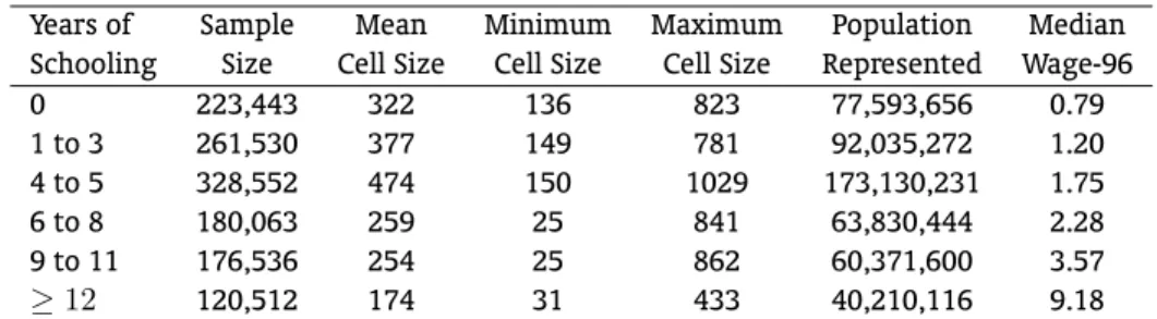
Table 1 –Cells Descriptions: 1977-1997
Years of Sample Mean Minimum Maximum Population Median Schooling Size Cell Size Cell Size Cell Size Represented Wage-96
0 223,443 322 136 823 77,593,656 0.79
1 to 3 261,530 377 149 781 92,035,272 1.20
4 to 5 328,552 474 150 1029 173,130,231 1.75
6 to 8 180,063 259 25 841 63,830,444 2.28
9 to 11 176,536 254 25 862 60,371,600 3.57
≥12 120,512 174 31 433 40,210,116 9.18
that finds that most of the differences in the returns to skill across countires can be explained by differences in supply shifts.
2. DATA DESCRIPTION
In this paper we use a particularly rich data set, consisting of repeated cross-sections of an annual household survey (PNAD), conducted each September by the Brazilian Census Bureau (IBGE). Each cross-section is a representative sample of the Brazilian population and contains about 100,000 observations on households, from which around 330,000 individuals are interviewed. From the original data we kept only males (to avoid the usual composition problems associated with changes in female participation), with positive hours worked in the reference week, positive monetary remuneration and between 24 and 56 years of age.4 We split the sample into six education groups: illiterates (0 years of schooling), incomplete elementary (1 to 3), complete elementary (4 to 5), (at least some) secondary (6 to 8), (at least some) high school (9 to 11) and (at least some) college (higher than 12). Within each education group we further group the data into 693 cells (33 age groups and 21 years). The sample period ranges from 1977 to 1997 and the final sample sizes are set out in Table 1.5
The main variable used in this analysis is real hourly wage, defined as normal labor income in the main job in the reference month normalized by normal weekly working hours. The last column of Table 1 presents the median wage for each education group in 1996. As the numbers are approximately equivalent to American dollars,6one can note, first of all, the low wage levels prevailing in the Brazilian economy. In 1996, for example, about 75% of all Brazilian workers we earning less than the American minimum wage (U$4.76). Moreover, the difference in wages across educational levels seems remarkable as well, since the median college educated worker earns about 11 times more than the median illiterate and about two and a half times more than the median high school worker.
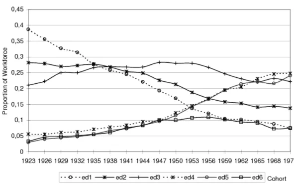
Figure 1 and 2 describe the evolution of the education composition of the Brazilian workforce, by plotting the percentage of each education group in the labor force across cohorts and over time. It is clear that meaningful changes across cohorts are taking place, that are reflected in the composition of the workforce over the sample period. Figure 1 depicts the big decline in the percentage of workers with no schooling (ed1), that represented 40% of the individuals born in 1923 and only about 8% of the
4We prefered to keep in the sample the self-employed and agricultural workers and those working in the informal sector of the economy.
5It is important to note that PNAD was not conducted in 1991 (census year) nor in 1994 (for budget reasons). We therefore interpolated the wage figures for these years within each education and age group using the adjacent years.
6The Brazilian Currency is the Real (R$). In October 1996, 1R$∼
=1US$, so that the figures can be interpreted as the hourly wage
Figure 1 –Education Composition by Cohort
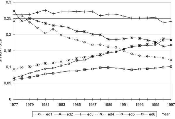
1971 cohort. The group with only basic reading and writing skills (ed2) also fell from 28% of the work-force to about 14% in the newest generation. The participation of the group with complete primary education has remained roughly constant, whereas a continuous increase was observed in the propor-tion of workers with secondary (ed4) and with high school educapropor-tion (ed5), these two groups jointly accounting for about 50% of the 1971 cohort composition. Interestingly, the proportion of workers with college education was increasing at the same rate of the high school group until the 1947 cohort, when it suddenly stopped growing. Figure 2 shows that these movements across generations are smoothed when plotted over time, since the different cohorts coexist at a point in time.
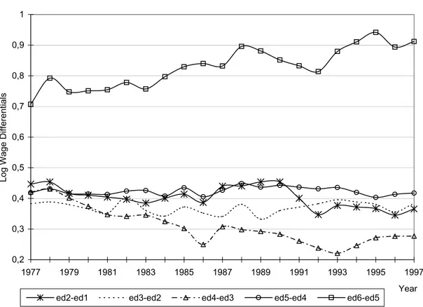
The differentials in mean (log) wage between each two successive education groups are plotted in figure 3.7 It seems that the price or “compression” effects were not as important as one might have expected, given the compositional changes described above. The most pronounced changes took place with the wage differential between the complete and incomplete elementary education (ed4-ed3), that fell markedly over the sample period and with the college wage differential (ed6-ed5), that rose continuously. It is important to note that, because the majority of the workers have 8 years or less of schooling in 1977 (72%), the workforce as a whole was much more affected by the drop in the complete elementary premium (ed4-ed3) than by the rise in college differential (ed6-ed5), which meant that average returns to education fell from 0.17 in 1977 to 0.14 in 1997.
To what extent have these changes in composition and in returns to education have impacted the evolution of the wage inequality in Brazil? In the next few sections, we will use econometric techniques to try and isolate the effects of education from cyclical, macroeconomic and experience effects.
0 0,05 0,1 0,15 0,2 0,25 0,3
1977 1979 1981 1983 1985 1987 1989 1991 1993 1995 1997
Year
% W
o
rk
Forc
e
ed1 ed2 ed3 ed4 ed5 ed6
Figure 2 –Education Composition over Time
Notes: ed1 = illiterates, ed2 = incomplete primary, ed3 = complete primary, ed4 = secondary ed5 = high school and ed6 = college education.
3. ECONOMETRIC METHODOLOGY
The evolution of wage inequality over time can be described by a framework that includes time, experience and cohort effects. The time (or macro) effects include changes in economic environment, such as institutional factors, inflation and unemployment rates that affect the workforce as a whole. Experience effects capture, for example, the impact of a wage dispersion that is increasing over the life-cycle, together with an aging population. Cohort effects reflect permanent changes in the composition of the population, due to differences in the characteristics of new entrants vis-a-vis leavers in the labor market (such as the size of the cohort and the level, quality and inequality of schooling).
Unfortunately, it is impossible to disentangle their separate effects, due to a fundamental identifi-cation problem. As Heckman and Robb (1985) point out, birth cohort(c)is completely determined by age(a)and a time trend(t):
c=t−a (1)
We try to model the wage equation in a parsimonious way, following MaCurdy and Mroz (1995), with functions of time, age and cohorts:
l(w) =α+A(a) +T(t) +C(c) +R(a, t, c) +u (2)
0,2 0,3 0,4 0,5 0,6 0,7 0,8 0,9 1
1977 1979 1981 1983 1985 1987 1989 1991 1993 1995 1997
Year
Log Wage Differentials
ed2-ed1 ed3-ed2 ed4-ed3 ed5-ed4 ed6-ed5
Figure 3 –Returns to Education Over Time
Notes: ed1 = illiterates, ed2 = incomplete primary, ed3 = complete primary, ed4 = secondary ed5 = high school and ed6 = college education.
time, age and possible interactions between the three, we know that, because of the identification problem, out of the 30 coefficients associated with fourth order terms, only 14 linear combinations can be identified. We therefore chose as the equation to be taken to the data:
l(w) =α+A1a+A2a 2
+A3a 3
+A4a 4
+T1t+T2t 2
+T3t 3
+T4t 4
(3)
+R1at+R2at 2
+R3a 2
t+R4a 3
t+R5t 3
a+R6a 2
t2+u
Hence, when interpreting the results of the regressions, it must be kept in mind that the cohort effects are present in the estimated coefficients. The error term in (3.3) include common time effects:
u=uit+ut (4)
that are constructed to be orthogonal to the age and trend functions, that is, include no trends. All trends in the data will be reflected in the age and trend variables.8
In the empirical investigation, we apply quantile regression techniques (Koenker and Basset, 1978). This allows us to model the evolution of the entire distribution of wages and not just the conditional mean. If all percentiles within a group evolve in the same way (apart form an intercept shift), then the
changing dispersion of wages can be explained by changing prices and/or composition of observed skill characteristics. Otherwise, unbsorved effects are also important. The median defines the location of the distribution and the percentiles around it describe the changes in dispersion. We therefore have:
l(w)q =
Aq(a) +Tq(t) +Rq(a, t) +uq (5)
The set of functionsTq(t)for each quantile measures the trends in wages over time. Differences in these functions between the top and bottom of the distribution capture drifts on wage dispersion within-groups. Differences in the estimated coefficients across education groups for the same quan-tile measure changes in the returns to education over time at specific points of the distribution. The functionsAq(a)measure describe the wage evolution as each education group gets older. Differences in the median age coefficient across education groups capture interactions between experience and education, whereas differences in the estimated age coefficients across quantiles would mean that the variance of wages increases with age, perhaps because of differential rates of learning by doing (see Gosling et al. 1999). Common macroeconomic shocks to the wage distribution are assumed to be the same for each educational group, regardless of age.
The procedure is as follows: the raw data is split into education, year and age cells, using the fact that the variables of interest are all discrete, and we choose within each cell a population characteris-tic of interest. We then estimated it with the corresponding sample characterischaracteris-tic (using the weights provided by the household surveys). We estimate the 1st, 5th,10th,15th,. . . , 90th, 95th and 99th per-centiles for each age, year and education cell. This is equivalent to using the full sample to regress each wage percentile on all possible education year and age interactions. The percentiles are asymptotically normally distributed (see Koenker and Portnoy, 1996). The variance of each of these estimated order statistic(q)is given by:
V(q) =q(1−q)
N f(q)2 (6)
We estimatef(q)(the conditional density) using a Gaussian Kernel with bandwith equal to half the standard deviation of wages for each cell.
We then try to impose some structure on the wage distribution by means of a minimum distance estimator. The minimum distance procedure choosesβsuch as to minimize:
(q−Zβ)V(q)−1(q−Zβ)
whereqis the estimated order statistic andZis a set of linear restrictions9. In our case, the restrictions imply that the age, trend and (orthogonal) time dummies can explain the behavior of each estimated order statistic across cells and over time. Imposing the restrictions means estimating weighted least squares regressions on the grouped data, for each quantile and education group separately. This proce-dure will give us consistent estimates ofβ.10 Under the null hypothesis that the restrictions are valid, the minimized value follows a chi-squared distribution with degrees of freedom equal to the number of restrictions. All we have to do to construct the test statistic is sum the weighted squared residuals, i.e. the empirical percentiles minus the age and trend effects, minus the orthogonal time effects.
4. RESULTS
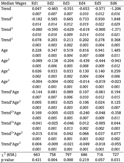
Tables 2 to 4 present the results of the median, 25th and 75th percentile regressions, respectively. One can note that the chi-square tests perform reasonably well in the median regressions, specially
9See Rothenberg (1971) and Chamberlain (1993).
Table 2 –Median Regression
Median Wages Ed1 Ed2 Ed3 Ed4 Ed5 Ed6
Trend 0.047 -0.465 -0.551 -0.653 -0.571 -1.206 0.007 0.007 0.007 0.010 0.012 0.016 Trend2
-0.182 0.585 0.665 0.733 0.930 1.848 0.014 0.014 0.012 0.019 0.022 0.029 Trend3
-0.080 -0.595 -0.629 -0.619 -0.900 -1.371 0.010 0.010 0.009 0.014 0.016 0.021 Trend4
0.078 0.203 0.213 0.202 0.278 0.368 0.003 0.003 0.002 0.003 0.004 0.005
Age 0.228 0.347 0.519 0.816 0.941 1.485
0.005 0.005 0.004 0.007 0.008 0.011 Age2
-0.089 -0.138 -0.204 -0.439 -0.444 -0.943 0.005 0.006 0.005 0.008 0.009 0.012 Age3
0.026 0.033 0.033 0.130 0.140 0.259 0.002 0.003 0.002 0.004 0.004 0.006 Age4
-0.004 -0.004 -0.002 -0.014 -0.019 -0.023 0.001 0.001 0.001 0.001 0.001 0.001 Trend*Age -0.144 0.081 0.089 0.107 -0.061 0.194 0.007 0.007 0.006 0.010 0.012 0.015 Trend*Age2
0.005 0.003 0.025 0.106 0.024 0.125 0.003 0.003 0.003 0.005 0.005 0.007 Trend2
*Age 0.169 -0.005 -0.025 -0.240 -0.048 -0.358 0.005 0.005 0.005 0.007 0.009 0.011 Trend3
*Age -0.041 -0.025 -0.046 0.012 -0.005 0.044 0.001 0.001 0.013 0.002 0.002 0.003 Trend2
*Age2
-0.015 0.016 0.042 0.066 0.037 0.077 0.001 0.001 0.001 0.001 0.002 0.002 Trend*Age3
0.004 -0.009 -0.021 -0.049 -0.018 -0.055 0.001 0.001 0.001 0.001 0.001 0.001
χ2
(658.) 663 758 797 686 716 727
p-value 0.431 0.004 0.000 0.219 0.057 0.031
Notes: Standard errors in italics
given the large degrees of freedom associated with the test. They fail to reject the restrictions in the median regression for the first, fourth and fifth educational level, while rejecting for the other three education groups.
The behavior of evolution of the 25th and 75th percentile are harder to predict, given that the restrictions were rejected in the majority of cases. It seems therefore that the functions (3.5) are best regarded as a convenient approximation to a more complex regression function (as in Chamberlain (1993), but see also the figures below).
Inspection of the estimated coefficients in Table 2 reveal some interesting features.11 First of all, there are meaningful differences in the estimated trend and experience effects across all the educational groups, revealing that returns to education were indeed changing in Brazil over the sample period and that returns to experience vary substantially across education levels. Additionally, the interactions
Table 3 –25th Quantile regression
25th Quantile Ed1 Ed2 Ed3 Ed4 Ed5 Ed6
Trend 0.037 -0.127 -0.324 -0.526 -0.445 -1.049 0.008 0.007 0.007 0.011 0.013 0.019 Trend2
0.191 0.029 0.091 0.339 0.515 1.665 0.015 0.013 0.012 0.020 0.024 0.035 Trend3
-0.611 -0.243 -0.210 -0.367 -0.580 -1.337 0.011 0.010 0.009 0.015 0.017 0.026 Trend4
0.255 0.125 0.115 0.159 0.205 0.382 0.003 0.003 0.002 0.003 0.004 0.006
Age 0.124 0.272 0.450 0.726 0.915 1.283
0.005 0.005 0.004 0.007 0.008 0.013 Age2
0.003 -0.109 -0.171 -0.397 -0.452 -0.694 0.006 0.006 0.005 0.008 0.010 0.015 Age3
-0.005 0.024 0.021 0.110 0.125 0.150 0.003 0.003 0.002 0.004 0.005 0.007 Age4
-0.001 -0.003 -0.001 -0.011 -0.013 -0.007 0.001 0.001 0.001 0.001 0.001 0.001 Trend*Age -0.074 -0.054 0.032 0.143 -0.058 0.291 0.007 0.007 0.006 0.011 0.012 0.018 Trend*Age2
-0.057 0.027 0.052 0.077 0.076 0.034 0.003 0.003 0.003 0.005 0.005 0.008 Trend2
*Age 0.177 0.074 -0.013 -0.183 -0.078 -0.336 0.005 0.005 0.005 0.008 0.009 0.013 Trend3
*Age -0.054 -0.043 -0.038 -0.017 -0.006 0.016 0.001 0.001 0.013 0.002 0.002 0.004 Trend2
*Age2
-0.005 0.015 0.033 0.069 0.038 0.094 0.001 0.001 0.001 0.001 0.002 0.002 Trend*Age3
0.013 -0.012 -0.022 -0.044 -0.032 -0.043 0.001 0.001 0.001 0.001 0.001 0.002
χ2
(658.) 774 623 843 744 740 840
p-value 0.001 0.823 0.000 0.010 0.014 0.000
Note: Standard errors in italics
between trend and age are significant, which could mean that returns to experience are changing over time and/or that cohort effects are important in Brazil.12
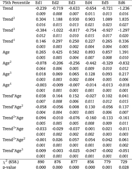
It is interesting to note that the differences in the coefficients across education levels also hold true for the other quantiles, as Tables 3 and 4 reveal. Moreover, there are marked differences between the estimated parameters across percentiles for the same education level, which indicates that important changes in the wage distribution within the education groups are taking place over time and over the life cycle in Brazil.
Table 4 –75th Quantile regression
75th Percentile Ed1 Ed2 Ed3 Ed4 Ed5 Ed6 Trend -0.239 -0.719 -0.633 -0.654 -0.721 -1.236
0.009 0.008 0.007 0.011 0.013 0.016 Trend2
0.304 1.188 0.930 0.903 1.089 1.835 0.016 0.015 0.013 0.021 0.023 0.027 Trend3
-0.384 -1.022 -0.817 -0.754 -0.927 -1.297 0.012 0.011 0.010 0.015 0.017 0.020 Trend4
0.146 0.297 0.250 0.227 0.265 0.336 0.003 0.003 0.002 0.004 0.004 0.005
Age 0.265 0.425 0.582 0.893 0.857 1.391
0.005 0.005 0.004 0.007 0.008 0.010 Age2
-0.078 -0.206 -0.256 -0.442 -0.329 -0.832 0.064 0.006 0.005 0.009 0.010 0.012 Age3
0.018 0.069 0.065 0.128 0.093 0.217 0.003 0.003 0.002 0.004 0.005 0.006 Age4
-0.003 -0.009 -0.007 -0.014 -0.013 -0.018 0.001 0.001 0.001 0.001 0.001 0.001 Trend*Age 0.038 0.164 0.152 -0.027 0.102 0.041 0.007 0.008 0.006 0.011 0.012 0.015 Trend*Age2
-0.058 -0.056 0.008 0.130 -0.056 0.137 0.004 0.004 0.003 0.005 0.006 0.007 Trend2
*Age 0.094 -0.010 -0.076 -0.160 -0.133 -0.161 0.005 0.005 0.005 0.008 0.009 0.011 Trend3
*Age -0.033 -0.029 -0.037 0.001 0.021 -0.011 0.001 0.002 0.002 0.002 0.003 0.003 Trend2
*Age2
-0.001 0.026 0.057 0.054 0.042 0.061 0.001 0.001 0.001 0.001 0.001 0.002 Trend*Age3
0.009 -0.003 -0.025 -0.047 -0.002 -0.051 0.001 0.001 0.001 0.001 0.001 0.001
χ2
(658.) 890 876 877 856 779 729
p-value 0.000 0.000 0.000 0.000 0.001 0.028
Note: Standard errors in italics
4.1. Fit of the Model
Besides the statistical tests, another procedure to evaluate the fit of the model and perform counter-factual experiments is to compare the observed unconditional wage distribution with the one pre-dicted by the restricted model. In order to construct the prepre-dicted wage distribution we proceed as in Gosling et al. (1999). We first construct the conditional wage distribution, by choosing a fixed numberwq (within the observed unconditional sample wage distribution ) and computing for each age/education/year cell (j):
Pr(w < wq|j) (7)
year:
q= Pr(w < wq) = j
fjPr(w < wq|j) (8)
wherefjis the observed cell frequency in the population.
With the unconditional wage distribution we can compute any inequality measure we need. In this paper we chose to work with the variance of (log) wages which, besides being much used in the literature, is one of the decomposable measures of inequality.13 Figure 4 shows, firstly, that the wage dispersion has remained basically stable over the last two decades, despite the fact that this was a period of very volatile macroeconomic conditions, especially between 1986 and 1992 when inflation accelerated to unprecedented levels. It also shows that the variance of labor earnings computed with the grouped data is permanently lower than the one calculated using the individual level information, a result that is expected since grouping eliminates some of the within-cell variability. More importantly however, is the fact that the variance computed using the restricted specification follows very closely the variance of the observed wages, so that the loss in precision occurs mainly from grouping.
0.6 0.7 0.8 0.9 1 1.1 1.2 1.3 1.4
1977 1979 1981 1983 1985 1987 1989 1991 1993 1995 1997
Year
V
a
r
(l
w
)
Grouped Data Predicted Individual Data
Figure 4 –Variance of Log (Labour Earnings)
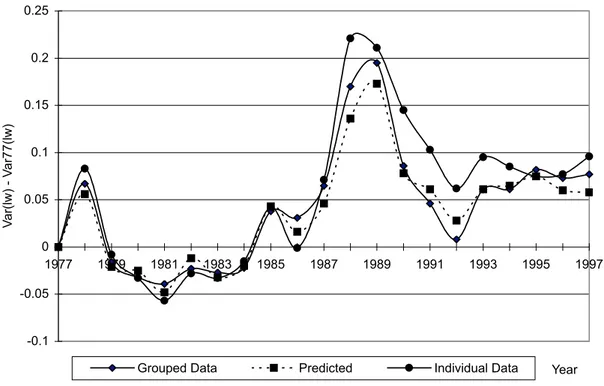
The evolution of the three measures of wage dispersion over time, measured as changes from the variance of wages in 1977, is described in Figure 5. The figure shows that the variance calculated from the restricted model closely mimics the behavior of the true variance, despite a period of short misalignment between 1989 and 1995. This means that we can use the predicted variance to construct counter-factuals and describe, for example, how inequality would look like had the returns to education remained at the 1977 level.
-0.1 -0.05 0 0.05 0.1 0.15 0.2 0.25
1977 1979 1981 1983 1985 1987 1989 1991 1993 1995 1997
Year
V
a
r(l
w
)
-
V
a
r7
7
(l
w
)
Grouped Data Predicted Individual Data
Figure 5 –Fit of the Model – Cumulative Changes
4.2. Variance Decomposition
We now use the predicted wage distribution to perform the usual variance decomposition with log wages(w):
V ar(wt) =
j
fjtV ar(wjt) +
j
fjt[E(wjt)−E(wt)] 2
(9)
where:
V ar(wjt) = E(w 2
jt)−[E(wjt)]
2
(10)
E(wjt) =
q
g(wq|j, t)wq
(11)
E(wt) =
q
g(wq)wq= q
[
j
fjtg(wq|j, t)]wq (12)
The empirical probability mass functiong(wq)was calculated using:
g(wq) =G(wq)−G(wq−ε) (13)
where:
G(wq) = Pr(w < wq) =q
period. In other words, the inequality of labor earnings in Brazil has risen slightly over the last two decades because of the dispersion within groups, that contributed to a fall in inequality in the first part of the 1980s followed by a substantial rise in the 1990s. The pattern of within group inequality closely followed the behavior of the inflation rates in the period and may be related to staggered wage contracts in periods of high inflation.14 What remains to be explained is why the between-group com-ponent of inequality failed to fall, despite the massive increase in education, accompanied by the fall in the economic returns to relatively low levels of education.
-0.1 -0.05 0 0.05 0.1 0.15 0.2
1977 1979 1981 1983 1985 1987 1989 1991 1993 1995 1997
Year
V
a
r(l
w
)
-
V
a
r7
7
(l
w
)
Predicted Within Groups Between Groups
Figure 6 –Variance Decomposition – Cumulative Changes
4.3. Counterfactual Analysis
As we saw above, the behavior of the variance of labor earnings can be decomposed into within-group and between-within-group components. Both these components are affected by the composition of the workforce, as the presence of (fjt) in equation (4.3) clearly demonstrates. Figure 7 plots the evolution of the within groups component after allowing the age structure within each education group to change, but maintaining the 1977 education configuration. It also depicts the behavior of the overall composi-tion effect, by keeping the age structure constant as well, that is, fixing all frequency weights (fj) in 1977.15
14The Brazilian Census bureau interviews individuals once a year, but in periods of rising inflation, wages are adjusted very frequently and at different times during the year. This may lead to ‘artificial’ rises in inequality measured at a point in time. 15The weights are computed using the cell sample size multiplied by the representativeness of each individual worker belonging
-0,08 -0,04 0 0,04 0,08 0,12 0,16
1977 1979 1981 1983 1985 1987 1989 1991 1993 1995 1997
Years
V
a
r(w
) - V
a
r77(w
)
Within Groups Constant Composition Const. Educ. Composition
Figure 7 –Within Groups Variance Component – Cumulative Changes
The figure reveals that the within group contribution to overall wage dispersion was predominantly the result of intra-cell dispersion and less due to the increasing importance of cells with higher disper-sion.16Changes in the composition of the workforce did not contribute very significantly to the cyclical variations in dispersion, but this effect has become more important in recent years. Moreover, the recent rise in importance of the composition effect is mainly due to education, since keeping the age structure also fixed (dotted line) has virtually no additional effect in the within-group component of inequality.
The evolution of the between-group contribution to inequality can be decomposed into a composi-tioneffect and acompressioneffect. Thecompressioneffect is evaluated by maintaining the composition of the population constant at its 1977 level, as we did with the within-group component above. There-fore, its behavior reflects the evolution of the difference between the mean wage within each cell and the overall sample mean. However, it is important to note at this point that the frequency weights have two roles in the between-group contribution to the variance of wages. Besides the role of measuring the ‘importance’ of each cell to the overall effect, they are also used to compute the overall (uncondi-tional) mean wage, as expression (4.6) reveals. Therefore, the compression effect is being driven by the difference between each group mean wage and the overall mean wage that would have prevailed had the structure of the population remained as in 1977.
Thecompositioneffect is obtained by maintaining the wage distribution within cells (and therefore their mean wage) at the 1977 level and allowing the frequency weights (fjt)to change. We do this by switching off the trend effects and their interactions with age for each education group, then pre-dicting the conditional wage distribution within each cell and using (4.6) to compute the unconditional distribution. The changes (fjt)also alter the between-groups contribution to inequality in two ways:
through changes in the weight of each cell’s wage deviation from the mean wage and through changes in the unconditional mean wage as well.
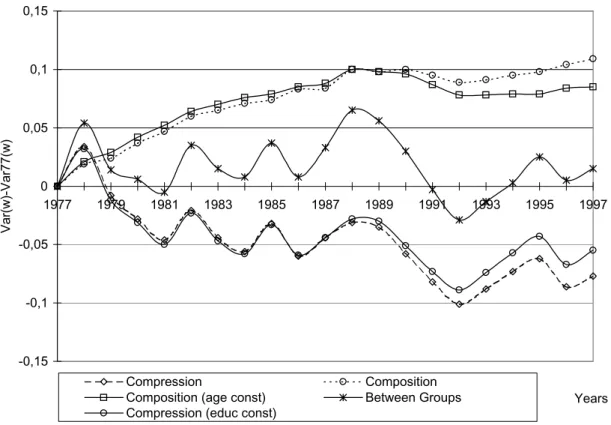
The evolution of the compression and composition effects over time is depicted in Figure 8, where the two components are shown to contribute very differently to the dispersion between groups. The fall in returns to low levels of education (compression effect) contributed to a significant reduction in between group inequality (of about 6%).17 Only a small part of the overall effect is due to age effects, since when we additionally keep the age composition of the workforce constant (dotted line) the behavior of the compression effect does not change very much.
-0,15 -0,1 -0,05 0 0,05 0,1 0,15
1977 1979 1981 1983 1985 1987 1989 1991 1993 1995 1997
Years
V
a
r(w
)-V
ar77(w
)
Compression Composition Composition (age const) Between Groups Compression (educ const)
Figure 8 –Between Groups Component – Cumulative Changes
On the other hand, the education composition effect followed in the opposite direction, increasing inequality by about 10%. It was the combination of these two opposite forces that led to the stability of the between-group dispersion, which, were it not for the composition effect, would be falling rapidly over the sample period. The figure also plots the total composition effect, that was obtained when we additionally held the age composition constant at 1977 (dotted lines with circles). The behavior of the two curves were every similar until 1992, when the contribution of the education composition showed a tendency to stabilize, whereas the overall composition effect continued to rise.
4.4. Simulations
From the above analysis, it seems that the education distribution has been impacting the evolu-tion of wage inequality in Brazil in a perverse way. This sub-secevolu-tion examines whether this impact
Table 5 –Predicted Education Distribution Education Group 2013 Cohort
Optimistic Pessimistic
Illiterates 0 % 2 %
Incomplete Elementary 0 % 8 % Complete Elementary 10 % 15 %
Secondary 30 % 30 %
High School 40 % 30 %
College 20 % 15 %
is predicted to change in the future, depending on the evolution of the education composition of the workforce. In order to simulate how this composition will look like in the next 40 years, we simulated the schooling structure of the share of the Brazilian workforce that will be between 24 and 56 years old in 2037. In order to do this, we predicted the education composition of each cohort between the one born 1981 and the one born 2013, based on the recent evolution of education across cohorts (figure 1). For instance, the predicted composition of the 2013 cohort under two alternative scenarios is set out in Table 5:
Based on these scenarios and using the 1997 age structure of the population, we predicted the education distribution of the workforce in 2037 and interpolated its evolution from 1997 to 2037. With these numbers at hand, we simulated how the composition effect would look like for the next 40 years, as figure 9 reveals. The composition effect is predicted to remain stable until 2007 under both scenarios, beginning to fall more rapidly between 2017 and 2017. Between 2017 and 2037 the difference between the two scenarios is more evident, with a substantial reduction in inequality occurring in the optimistic scenario, where inequality is predicted to return to its 1977 level by 2027 and drop even more by 2037. In the pessimistic scenario, inequality will return to the 1977 level by 2037.
One of the drawbacks of the present simulations is that they do not take into account the possibility of interactions between the composition and the compression effects, i.e., that the evolution of the returns to education over time might either accelerate or delay the drop in the between-groups com-ponent of wage dispersion. The dotted line in figure 9 depicts the predicted composition effect, under the pessimistic scenario, with the wage distribution fixed in 1997 instead of 1977.18 It shows that the predicted composition impact is virtually the same with 1997 prices, which means that the prediction is robust to different initial wage distributions.
5. CONCLUSIONS
In this paper we investigated the behavior of the distribution of male wages in Brazil in the 1980s and 1990s. The results showed that overall inequality remained basically unaltered over this period, primarily due to the stability of wage dispersion between groups. Counterfactual experiments showed that this stability was the result of two forces acting in opposite directions. The compression effect (returns to education) induced a reduction in dispersion, whereas the composition effect contributed to a rise in inequality. Simulations using the predicted evolution of the education distribution of the workforce indicated that the composition effect will start contributing to a decline in inequality in about 10 years time. Future work will indicated whether the results obtained here apply solely to the Brazilian case or can be generalized to other less developed countries.
-0,06 -0,04 -0,02 0 0,02 0,04 0,06 0,08 0,1
1977 1987 1997 2007 2017 2027 2037
Year
V
a
r(w
) - V
a
r77(w
)
Pessimistic Scenario Optimistic Scenario Pessim -1997 prices
Figure 9 –Predicted Composition Effect
Bibliography
(2000).Human Development Report. United Nations Development Programe.
Barros, R., Henriques, R., & Mendonça, R. (2000). Education and equitable economic development. Economia, 1:111–144.
Beaudry, P. & Green, D. (1997). Cohort patterns in canadian earnings: Assessing the role of skil premia in inequality trends. Technical Report 163, National Bureau of Economic Research.
Chamberlain, G. (1993). Quantile regressions, censoring and the structure of wages.Advances in Econo-metrics, 1.
Chiswick, B. (1971). Earnings inequality and economic development. Quarterly Journal of Economics, 85:21–39.
Ferreira, F. H. G. & de Barros, R. P. (1999). The slippery slope: Explaining the increase in extreme poverty in urban brazil; 1976–1996.Revista de Econometria, 19(2):211–296.
Fields, G. (1980).Poverty, Inequality and Development. Cambridge University Press, New York.
Gosling, A., Machin, S., & Meghir, C. (1999). The changing distribution of male wages in the UK. Technical Report 271, Centre for Economic Performance.
Heckman, J. & Robb, R. (1985). Using longitudinal data to estimate age, period and cohort effects in earnings equations. In Feinberg & Mason, editors,Analysing Longitudinal Data for Age, Period and Cohort Effects. Academic Press, New York.
Knight, J. & Salbot, R. (1983). Education expansion and the kuznets effect. American Economic Review, 73:1132–1136.
Koenker, R. & Basset, G. (1978). Regression percentiles.Econometrica, 46:33–50.
Koenker, R. & Portnoy, S. (1996). Quantile regression. Technical Report 97–0100, University Illinois, Urbana-Champaign.
Kuznets, S. (1955). Economic growth and income inequality.American Economic Review, 45:1–28.
MaCurdy, T. & Mroz, T. (1995). Estimating macro effects from repeated cross-sections. Technical report, University of Standford.
Ram, R. (1990). Education expansion and schooling inequality: International evidence and some impli-cations.Review of Economics and Statistics, 72:266–274.
Rothenberg, T. (1971).Efficient Estimation with A Priori Information. Yale University Press, New Haven.