❊♥s❛✐♦s ❊❝♦♥ô♠✐❝♦s
❊s❝♦❧❛ ❞❡
Pós✲●r❛❞✉❛çã♦
❡♠ ❊❝♦♥♦♠✐❛
❞❛ ❋✉♥❞❛çã♦
●❡t✉❧✐♦ ❱❛r❣❛s
◆◦ ✻✵✵ ■❙❙◆ ✵✶✵✹✲✽✾✶✵
■♠♣❡r❢❡❝t❧② ❈r❡❞✐❜❧❡ ❉✐s✐♥✢❛t✐♦♥ ✉♥❞❡r ❊♥✲
❞♦❣❡♥♦✉s ❚✐♠❡✲❉❡♣❡♥❞❡♥t Pr✐❝✐♥❣
❈❛r❧♦s ❱✐❛♥❛ ❞❡ ❈❛r✈❛❧❤♦✱ ▼❛r❝♦ ❆♥tô♥✐♦ ❈❡s❛r ❇♦♥♦♠♦
❖s ❛rt✐❣♦s ♣✉❜❧✐❝❛❞♦s sã♦ ❞❡ ✐♥t❡✐r❛ r❡s♣♦♥s❛❜✐❧✐❞❛❞❡ ❞❡ s❡✉s ❛✉t♦r❡s✳ ❆s
♦♣✐♥✐õ❡s ♥❡❧❡s ❡♠✐t✐❞❛s ♥ã♦ ❡①♣r✐♠❡♠✱ ♥❡❝❡ss❛r✐❛♠❡♥t❡✱ ♦ ♣♦♥t♦ ❞❡ ✈✐st❛ ❞❛
❋✉♥❞❛çã♦ ●❡t✉❧✐♦ ❱❛r❣❛s✳
❊❙❈❖▲❆ ❉❊ PÓ❙✲●❘❆❉❯❆➬➹❖ ❊▼ ❊❈❖◆❖▼■❆ ❉✐r❡t♦r ●❡r❛❧✿ ❘❡♥❛t♦ ❋r❛❣❡❧❧✐ ❈❛r❞♦s♦
❉✐r❡t♦r ❞❡ ❊♥s✐♥♦✿ ▲✉✐s ❍❡♥r✐q✉❡ ❇❡rt♦❧✐♥♦ ❇r❛✐❞♦ ❉✐r❡t♦r ❞❡ P❡sq✉✐s❛✿ ❏♦ã♦ ❱✐❝t♦r ■ss❧❡r
❉✐r❡t♦r ❞❡ P✉❜❧✐❝❛çõ❡s ❈✐❡♥tí✜❝❛s✿ ❘✐❝❛r❞♦ ❞❡ ❖❧✐✈❡✐r❛ ❈❛✈❛❧❝❛♥t✐
❱✐❛♥❛ ❞❡ ❈❛r✈❛❧❤♦✱ ❈❛r❧♦s
■♠♣❡r❢❡❝t❧② ❈r❡❞✐❜❧❡ ❉✐s✐♥❢❧❛t✐♦♥ ✉♥❞❡r ❊♥❞♦❣❡♥♦✉s ❚✐♠❡✲❉❡♣❡♥❞❡♥t Pr✐❝✐♥❣✴ ❈❛r❧♦s ❱✐❛♥❛ ❞❡ ❈❛r✈❛❧❤♦✱
▼❛r❝♦ ❆♥tô♥✐♦ ❈❡s❛r ❇♦♥♦♠♦ ✕ ❘✐♦ ❞❡ ❏❛♥❡✐r♦ ✿ ❋●❱✱❊P●❊✱ ✷✵✶✵ ✭❊♥s❛✐♦s ❊❝♦♥ô♠✐❝♦s❀ ✻✵✵✮
■♥❝❧✉✐ ❜✐❜❧✐♦❣r❛❢✐❛✳
Imperfectly Credible Disin
fl
ation under Endogenous
Time-Dependent Pricing
∗
Marco Bonomo
Graduate School of Economics, Getulio Vargas Foundation and CIREQ
Carlos Carvalho
Federal Reserve Bank of New York
August 2007
Abstract
The real effects of an imperfectly credible disinflation depend critically on the extent of price rigidity. Therefore, the study of how policymakers’ credibility affects the outcome of an announced disinflation should not be dissociated from the analysis of the determinants of the frequency of price adjustments. In this paper we examine how credibility affects the outcome of a disinflation in a model with endogenous time-dependent pricing rules. Both the initial degree of price ridigity, calculated optimally, and, more notably, the changes in contract length during disinflation play an important role in the explanation of the effects of imperfect credibility. We initially evaluate the costs of disinflation in a setup where credibility is exogenous, and then allow agents to use Bayes rule to update beliefs about the “type” of monetary authority that they face. In both cases, the interaction between the endogeneity of time-dependent rules and imperfect credibility increases the output costs of disinflation, but the pattern of the output path is more realistic in the case with learning.
JEL classification: E31; E52
∗This paper was previously entitled “Endogenous Time-Dependent Rules and the Costs of Disinflation
with Imperfect Credibility.” We thank the participants at the Latin American Meeting of the Econometric Society, “Microeconomic Pricing and the Macroeconomy” workshop at CEU, and workshops at EPGE-FGV, Princeton, PUC-Rio, Queen Mary - University of London, UIUC, Universidade Nova de Lisboa, and Université de Montreal, for helpful comments. Marco Bonomo would like to thank the Bendheim Center for Finance, Princeton University, for hospitality, and CAPES (Ministry of Education, Brazil) forfinancial
support. Carlos Viana de Carvalho gratefully acknowledgesfinancial support while at Princeton University.
1
Introduction
Lack of credibility has, for a long time, been pointed out as an important ingredient in explaining real effects of disinflation (e.g. Sargent, 1983). It arises when a monetary authority
that is serious about disinflating faces distrust from the private sector. Yet, price rigidity
is necessary for an imperfectly credible disinflation to have real effects. If prices are fully flexible, monetary policy essentially has no real effects, and the lack of credibility does not
matter.1
Additionally, the extent of price rigidity matters for the effect of imperfect credibility. Consider an economy during an imperfectly credible disinflation in which individual prices are fixed for extremely short periods of time. Then, the price optimally set by eachfirm will tend
to be very similar to the price that would be set under full credibility, since there is relatively little uncertainty about the monetary policy regime in the very short run. Therefore, the real effect of imperfect credibility will not be very important. However, the same will not be true for an economy where prices are fixed for long periods. Since policy uncertainty tends
to build up with time, there will be a much higher probability of a policy reversal during this longer time period. This uncertainty will affect pricing decisions, leading to substantial differences between the individual prices set during an imperfectly credible and a perfectly credible disinflation.2
Because the role of credibility depends on the frequency of price changes, conclusions about the effect of imperfect credibility that are based on models where this frequency is chosen arbitrarily will reflect this arbitrary choice. In addition, since a disinflation typically
involves a policy regime change, analyses based on such models are subject to the Lucas critique. Not only should the degree of price rigidity respond to the change in regime, it should also depend on its credibility. For those reasons, the study of the role of credibility in disinflation episodes should not be dissociated from the analysis of the determinants of
the frequency of price changes.
In this paper, we analyze how a policymaker’s credibility affects the outcome of a dis-inflation in a model with endogenous price rigidity. In our model firms face frictions that
make it optimal to choose ex-ante the time of the next price change. As a result the time period between price adjustments, or contract length, responds to changes in the economic
1In standard models with one equilibrium. Of course, in a model with multiple equilibria, credibility, as sunspots, may move the economy from one equilibrium to another.
environment.
Credibility affects the costs of disinflation through a direct and an indirect effect on
prices. The direct effect is through the expectation of marginal costs during a given contract length, and appears in other models based on exogenous time-dependent pricing rules (e.g. Ball 1995, and Erceg and Levin 2003). As we argued above, the magnitude of this effect hinges on the duration of price contracts. Our framework naturally brings discipline to the analysis, since contract lengths are determined endogenously.3 The indirect effect arises
in our model with endogenous pricing rules because changes in contract length during the disinflation also affect the individual prices chosen. With policy regime shifts, as it happens
with a new disinflationary policy, this effect becomes important.
In Section 2 we derive the optimal pricing rules under the assumption thatfirms cannot
obtain, process and react to new informationnor adjust prices based on their old information unless they incur a lump sum cost, as in Bonomo and Carvalho (2004). We extend their approach to derive optimal pricing rules during an imperfectly credible disinflation. The
resulting pricing rules are endogenous time-dependent rules, where each time a firm incurs
the information/adjustment cost, it sets a price and chooses ex-ante when next to gather and process information and set a new price. We refer to such chosen times as pricing dates.4
We view the assumption of a single information/adjustment cost as a tractable way to incorporate information frictions and adjustment costs that appear to be present in price setting decisions, as documented by Zbaracki et al. (2004). The resulting pricing rules display time dependency that resembles the “pricing seasons” described by those authors, and nominal rigidities that are consistent with microeconomic evidence on individual prices (e.g. Bils and Klenow 2004 for recent evidence for the U.S. economy). Moreover, endogenous time-dependency implies a frequency of price changes that increases with inflation, in line
with both time-series and cross-country evidence (e.g. Dhyne et al. 2006, Gagnon 2006, Konieczny and Skrzypacz 2005, Lach and Tsiddon 1992, and Nakamura and Steinsson 2007). Our main interest is to analyze the mechanism through which imperfectly credible dis-inflations affect output in a setting in which price setting decisions are optimal. We take
credibility as exogenous, and model imperfect credibility as the discrepancy between private
3One could argue that the arbitrariness in specifying (exogenous) contract lengths could be avoided by calibrating the frequency of price changes to the microeconomic evidence. However, this would restrict the scope of analysis to economic environments similar to the ones that produced the evidence used in the calibration. In contrast, our approach allows us to calibrate the primitive parameters of the model to the available evidence, and compute contract lengths for different economic environments.
agents’ beliefs about the likelihood that the monetary authority abandons the disinflation,
and the objective likelihood. Such beliefs affect aggregate outcomes through their effect on the choice of contract lengths, and prices set byfirms.5
In Section 3 we examine the case where, despite price setters’ beliefs, there is no policy reversal. We evaluate the output effects under exogenous and endogenous pricing rules. Our exogenous rules feature contract lengths which are chosen optimally for the inflationary
environment which prevailed before the disinflation was launched. Thus, we appropriately
measure the direct effect of credibility by comparing the output effects of disinflation under
perfect and imperfect credibility in different economic environments. Imperfect credibility increases disinflation costs because agents believe that there is some probability that the
stabilization will be abandoned before their next pricing date, and therefore set prices higher than in the full credibility case.
In order to assess the indirect effect of credibility, we examine the case in which pricing rules are endogenous, and compare it with the exogenous pricing rules case. We find that
endogeneity of time-dependent rules increases the costs of imperfectly credible disinflation.
The intuition underlying the result is as follows. With endogenous rules, firms optimally
choose longer contract lengths while the stabilization is maintained, since expected inflation
is lower. This raises the probability of a policy reversal occurring before the next pricing date, amplifying the difference between individual prices set under perfect and imperfect credibility. Endogeneity of pricing rules and imperfect credibility interact to generate an additional effect on top of the effects entailed by the endogeneity of rules under perfect credibility (Bonomo and Carvalho, 2004), and by imperfect credibility under exogenous rules (Ball, 1995).
In Section 4 we introduce learning. The assumption that agents do not learn, despite useful for gaining insight, is not realistic. It generates the unappealing result that a certain level of recession goes on indefinitely. One should expect the monetary authority to gain
credibility through time, as agents update their beliefs about its resolve by observing that disinflation continues. We endogenize the evolution of agents’ beliefs through Bayesian
learning. The result is a more realistic output path in which the monetary authority gains credibility, and the recession is gradually eliminated. Moreover, the main result of the paper, that endogeneity of pricing rules and lack of credibility interact to generate higher disinflation
costs, continues to hold.
The literature that links imperfect credibility and price rigidity explicitly starts with Ball
5There is another line of investigation about the effects of imperfect credibility on disin
flation, which
(1995), who argues that both ingredients are necessary to explain the costs of disinflation.
He focuses on average effects of disinflation when agents’ beliefs are in fact correct (i.e.
they know the distribution of abandonment times). Erceg and Levin (2003) explain the output costs during the Volcker disinflation with a model where agents have to learn about a
structural change in the interest rate rule. Both papers use exogenous pricing rules. Nicolae and Nolan (2006) model a credibility problem similar to ours, but have limited endogeneity of pricing rules: either prices are adjusted every period or every other period. They also introduce learning, but avoid Bayesian updating and, instead, experiment with alternative simple learning schemes. Finally, Almeida and Bonomo (2002) analyze the effect of imperfect credibility using models of endogenous, state-dependent pricing rules. However, since price setters observe monetary policy continuously, imperfect credibility only has effect through the changes in pricing rules, and the real output effects are muted.
2
The model
We start from a model with a representative consumer who derives utility from a Dixit-Stiglitz composite of different varieties of a consumption good. She incurs disutility from supplying all types of differentiated labor to a continuum of monopolistically competitive
firms, which are divided into industries.6 Labor markets are industry-specific, and each of
them is competitive. All firms in a given industry adjust prices at the same time, and are
subject to common productivity shocks. Each firm uses labor of the appropriate type to
produce a specific variety of the consumption good. As is now common in the literature, we
assume a cashless economy (e.g. Woodford 2003).
In Appendix A we develop the model from fundamentals, and derive the following log-linear expression for the frictionless optimal individual price of afirm in industry j, pjt:
pjt = (1−γ)pt+γ(Yt−ytn) +ejt, (1) whereptis the (log) aggregate price level,Ytis the (log) nominal aggregate demand,ynt is the (log) natural output rate. The ejt’s are mutually independent, zero mean industry-specific
shocks.
In (1), 1−γ is the degree of strategic complementarity in price setting, and is related
to primitive parameters such as the elasticity of substitution between varieties of the con-sumption good, and the intertemporal elasticity of substitution (see Appendix A). Individual
prices are strategic complements (substitutes) if γ <1 (>1). Complementarities may arise because segmentation in labor markets introduces real rigidities in the economy (Ball and Romer, 1990).
In order to find the aggregate price in a frictionless equilibrium, we integrate (1) across
allfirms:
pt =
Z 1
0
pjtdj =Yt−ytn.
Thus, in such equilibrium, aggregate output and individual prices are given by yn t and
pjt =pt+ejt, respectively.
For simplicity, in the subsequent sections we abstract from aggregate shocks, which im-plies that natural output is constant. Thus, all variation of the output level will be attributed to output gap variation as a result of price rigidity.
2.1
Optimal time-dependent pricing rule
The microeconomic evidence on nominal price rigidity has usually been rationalized by the existence of menu costs of changing prices. As it is well known, this leads to pricing decisions that are state-dependent. More recent work relying on interview studies (Blinder et al. 1998) and direct measurement through field work (Zbaracki et al. 2004) shows the importance of
other types of costs associated with price setting decisions, such as information gathering, decision making, and internal communication costs. Those costs prevent the continuous information gathering and processing that are necessary for the implementation of purely state-dependent pricing strategies.
Information and decision making costs lead to infrequent pricing decisions (Reis 2006), thus introducing elements of time dependency. However, in the absence of adjustment costs, the optimal pricing rules call for the choice of a price path at each decision date. Those rules are at odds with the microeconomic evidence on nominal price rigidity.
A model endowed with both information and adjustment costs should capture the time dependency uncovered in recent work (e.g. the pricing seasons documented in Zbaracki et al. 2004) and at the same time generate nominal price rigidity. A tractable model with these features was introduced by Bonomo and Carvalho (2004), wherefirms cannot obtain,
process and react to new informationnor adjust prices based on their old information unless they incur a lump sum cost. Here we adopt their approach and extend it to obtain optimal pricing rules in the presence of an imperfectly credible disinflation.
Every time a firm decides to gather and process information and/or adjust its price it
optimal pricing policy amounts to choosing a sequence of pricing dates. At each such date thefirm decides on the next pricing date and sets a price that will befixed until then.7 The
choice of the optimal time interval between pricing dates weights the benefits of updating
information and changing prices frequently against the pricing cost.
For analytical tractability we postulate thatfirmj chooses its pricing strategy by solving
the following problem:8
e
V (st) = min z,τ Et
∙Z τ
0
θ(θ−1)
2 (z−(pjt+u−pjt))
2
e−ρudu+e−ρτ ³Fe+Ve(st+τ)
´¸
. (2)
Here,θ >1is the elasticity of substitution between the varieties of the consumption good,Fe
is the pricing cost, τ denotes the time until the next pricing date, zt≡xjt−pjt denotes the discrepancy between the (log) price set at t, xjt, and its (log) frictionless optimal level pjt, and θ(θ−1)
2 (zt−(pjt+u−pjt))
2 is a second order approximation of the percentage of pro
fits
lost for not charging the frictionless optimal price at t + u.9 The relevant state of the
economy is denoted by st, with jth component sjt, and its law of motion is described by
st+∆t =Ω
¡
st, ηt,t+∆t
¢
, where ηt,t+∆t is the set of innovations that hit the economy between
t and t+∆t. The state of the economy matters for flow values through its effect on the
distribution of future frictionless optimal prices before the next pricing date (pjt+u for 0<
u < τ).
Defining L(st, u, z) ≡Et[z−(pjt+u−pjt)]2, a normalized expected profit loss, and F ≡
2Fh
θ(θ−1), a normalized pricing cost, the pricing problem can be rewritten as:
V (st) = min z,τ
∙Z τ
0
L(st, u, z)e−ρudu+e−ρτ(F +Et[V (st+τ)])
¸
. (3)
The first order conditions for the above problem are:
z∗(st) =
ρ
1−eρτ∗(st)
Z τ∗(st)
0
e−ρuEt(pjt+u −pjt)du, (4)
7One should note that in this setting any new information that becomes available to the firm is not taken into account until the next pricing date. This is also a feature of the inattention model of Reis (2006). The idea, in line with the evidence in Zbaracki et al. (2004), is that processing and deciding on the new information are costly activities.
8We omit thej subscript from choice variables to simplify notation. 9This approach is not fully structural. The quadratic loss
flow has a structural interpretation under a
linear production function, but the dynamic problem as a whole is not derived formally fromfirst principles.
and
L(st, τ∗(st), z∗(st))−ρF−ρEtV
¡
st+τ∗(st)¢+Et
"
∂V ¡st+τ∗(st)¢
∂s ·
∂Ω¡st, ηt,t+τ∗(st)
¢
∂τ
#
= 0,
(5) and the envelope conditions with respect to the components of st are:
∂V (st)
∂sjt =
"Z τ∗(st)
0
∂L(st, u, z∗(st))
∂sjt
e−ρudu
#
+e−ρτ∗(st)E
t
Ã
∂V ¡st+τ∗(st)
¢
∂s ·
∂Ω¡st, ηt,t+τ∗(st)¢
∂sjt
!
Equations (3), (4), and (5) together with the envelope conditions fully characterize the optimal pricing rule, as long as the second order conditions are satisfied. Thefirst equation
gives the optimal discrepancy for a given contract length. It should be set equal to a weighted average of expected increments in the frictionless optimal price during the contract. The second equation characterizes the optimal contract length, given the optimal discrepancy. It states that the expected marginal profit loss from postponing the next pricing date (the first term) should be equal to the marginal benefit of postponing the payment of the pricing
cost (the second term) and the expected cost of future cycles (the third term). The last term captures the marginal effect of postponing the next pricing date on the value function, through its effect on the future state of the economy.
2.2
In
fl
ationary steady state
In analyzing disinflations we start from an inflationary steady state characterized by a
con-stant rate of inflation. Let µ be the constant growth rate of nominal aggregate demand. If
we differentiate equation (1), and use the assumption of constant natural output rate, and the fact that in steady state all prices grow at the same rate, we obtain:
dpjt =µdt+dejt. (6) Realistically we think of the idiosyncratic productivity processes ej as being persistent, but stationary processes.10 However, modeling them as mean-reverting processes would add
a state variable to thefirm’s problem without changing the main insights regarding aggregate
dynamics. Thus, we adopt the Brownian motion as a convenient approximation of short run dynamics, that is:
dejt =σdWjt,
where Wjt’s are mutually independent standard Brownian motions. Given these assumptions, the Bellman equation (3) becomes:
Vµ= min z,τ Et
∙Z τ
0
(z−(pjt+s−pjt))2e−ρsds+e−ρτ(F +Vµ)
¸
, (7)
whereVµ represents the (constant) value function for the steady state problem with nominal aggregate demand growth rate equal toµ. In steady state, the value function and the optimal z andτ are the same for all firms, because they depend on the parameters of the stochastic
process for pj and not on its realizations.
The first order conditions (4) and (5) become:
z∗ = ρ 1−e−ρτ∗
Z τ∗
0
Et(pjt+s−pjt)e−ρsds; (8)
Et[z∗−(pjt+τ∗−pjt)]2−ρ(Vµ+F) = 0. (9) Manipulating (6), (7), (8), and (9), we arrive at the following equations, which defineτ∗ implicitly, andz∗:
ρ
Rτ∗
0 µ
µ2³h1
ρ− e−ρτ∗
1−e−ρτ∗τ∗
i
−s´2+σ2s 
e−ρsds+F
1−e−ρτ∗ =µ
2 µ
1
ρ−
e−ρτ∗
1−e−ρτ∗τ∗−τ∗
¶2
+σ2τ∗;
z∗ =µ
µ
1
ρ −
e−ρτ∗
1−e−ρτ∗τ∗
.
Based on the above pair of equations, one can show that the optimal contract length is decreasing in |µ| and σ, increasing in F, and is not affected by the degree of strategic
complementarity, 1−γ. In addition, higher idiosyncratic uncertainty makes the optimal
contract length less sensitive to inflation (Bonomo and Carvalho 2004).
In our simulations, we set σ = 3% and calibrate F in such a way that with µ = 3%,
σ = 3% and ρ= 2.5%a year, firms make pricing decisions once a year. As a result we set
F = 0.000595. This frequency of price changes seems to be a reasonable characterization of price setting behavior in low inflation environments. It is consistent with the findings
of Dhyne et al. (2006) for the Euro area, and with earlier evidence for the U.S. economy (e.g. Carlton, 1986 and Blinder et al., 1998), although it is lower than the frequency of price changes reported by Bils and Klenow (2004) for the U.S. economy.
confronted with the Israeli experience reported by Lach and Tsiddon (1992), and it also fits
the Brazilian hyperinflation experience of the 80’s (Ferreira, 1994). With inflation rates of
77% per year the model predicts contract lengths of 2.6 months, against 2.2 months reported by Lach and Tsiddon (1992), and with annual inflation of 210% the theoretical contract
length goes down to 1.68 months, against 1.38 months reported by Ferreira (1994). Thus, in accounting for the effects of inflation on the frequency of price changes the performance
of our endogenous time-dependent model is comparable to that of the menu cost model analyzed by Golosov and Lucas (2007).
2.3
Optimal pricing rule under imperfectly credible disin
fl
ation
In this subsection we derive optimal pricing rules during disinflation. In general, this requires
solving both an optimization and an aggregation problem simultaneously: the optimal pricing rule depends on the expected path for the aggregate price level, which in turn results from the aggregation of the individual rules. In the absence of strategic complementarities (γ = 1) these problems can be solved sequentially.
We simplify the analysis by assuming away strategic complementarities. This is a common assumption in state-dependent pricing models, where aggregation can be cumbersome (e.g. Caplin and Leahy 1991, Almeida and Bonomo 2002, and Golosov and Lucas 2007).11 In
terms of primitives of our model this obtains if, for instance, utility is logarithmic, and both the disutility of labor and technology are linear.12
The dynamic program formulated in (3) encompasses imperfect credibility in general, which enters the problem through the expectations operator. It is more realistic to assume that agents believe that there is some probability that the new disinflation policy will be
abandoned, than to assume full credibility. We model imperfect credibility by positing that in eachfinite time interval agents attribute a constant probability of a policy reversal. Thus,
from the agents’ perspective, the growth rate of nominal aggregate demand after the new policy is implemented changes with the first arrival of a Poisson process with constant rate
h. In case the disinflation is abandoned, agents believe that the old policy is resumed and
maintained forever.
Despite agents’ beliefs, we assume in this section that the monetary authority never reneges. Therefore, after the stabilization policy is launched at t= 0, the actual process for
11Caplin and Leahy (1997), and Gertler and Leahy (2006) are two noticeable exceptions.
nominal aggregate demand, Yt, is given by:
dYt = µ0dt;
Y0 = 0,
where µ0 is the targeted growth rate for nominal income, and where we introduced the
normalizationY0 = 0. We refer to the case of µ0 = 0 as “full disinflation,” whileµ > µ0 >0
corresponds to a “partial disinflation.” We implicitly assume that the monetary authority
sets its policy instrument so as to generate the postulated disinflation path for nominal
aggregate demand.
However, nominal aggregate demand according to agents’ beliefs, Yb
t, evolves as:
dYtb = (µ0+ (µ−µ0) 1{Nt>1})dt;
Y0b = 0,
whereNt is a Poisson counting process with constant arrival rateh, and1{·} is the indicator
function.
With this formulation we can interpret h as a measure of credibility, with high values
representing low credibility. The subjective probability that stabilization will last until time
T is given by e−hT. Thus, for example, if h = 0.5 (at an annual rate), the subjective probability that the stabilization will continue after one year is 61%. The polar cases of perfect and no credibility correspond to h= 0 andh=∞, respectively.
The fact that we model the frictionless optimal price as a random walk, together with the assumption that policy reversals arrive according to a constant hazard process simplify the pricing problem substantially. The relevant state after the disinflation is launched can
be summarized by a binary variable that indicates whether disinflation has been abandoned
or not. If a policy reversal has occurred, the pricing problem becomes identical to that of the inflationary steady state. Otherwise, the problem of a firm on a pricing date may be
written as:
Vh = min z,τ
£
Gh(z, τ) +e−ρτ
¡
F +e−hτVh+
¡
1−e−hτ¢Vµ
¢¤
, (10)
where
Gh(z, τ) ≡ e−hτ
∙Z τ
0 ³
(z−µ0s)2 +σ2s´e−ρsds
¸
+ (11)
Z τ
0
" Rr 0
¡
(z−µ0s)2
+σ2s¢e−ρsds+
Rτ r
¡
(z−µ(s−r)−µ0r)2
+σ2s¢e−ρsds
#
In (10), Gh(z, τ) is the expected cost due to deviations from the frictionless optimal price during the next interval of length τ, starting with the discrepancy z. Observe that if abandonment occurs during the next contract, agents will not learn of it until the new pricing date.13 Then, the new pricing decision will be made under conditions identical to
the inflationary steady state. This results in the cost function Vµ. In (11), the first line of
the expression refers to the subjective probability that the stabilization will be kept during the next interval of length τ multiplied by the cost in this case. The second line is the
discrepancy cost if abandonment occurs at timet+r weighted by the (subjective) likelihood
of this event.
The first order conditions are derived in a straightforward way:
z∗ = ρ 1−e−ρτ∗
Z τ∗
0 ∙
µ0s+ (µ−µ0)
µ
s−1−e−hs
h
¶¸
e−ρsds; (12)
(z∗−µ0τ∗)2+σ2τ∗+he−hτ∗(Vµ−Vh)−ρF −ρ
¡
e−hτ∗Vh+
¡
1−e−hτ∗¢Vµ
¢
(13)
+
Z τ∗
0
((µ0 −µ) (τ∗−r))2he−hrdr+ 2 (µ0−µ) (z∗−µ0τ∗)
Z τ∗
0
(τ∗−r)he−hrdr= 0.
From (12), (13), (10), (11) and (7), we obtain a nonlinear equation in τ∗, which can be solved numerically.
Figure 1 shows the optimal contract length as a function of the credibility level in a full disinflation, for two levels of initial inflation (µ= 0.1 andµ= 0.2). It shows that the lower the credibility level is (the higher h), the shorter the contract length is. A lower level of
credibility implies higher expected inflation, increasing the expected profit loss from having
a fixed price for a given contract length. Thus, if the contract length is unchanged, the
expected marginal loss at the next pricing date will exceed the expected marginal benefit of
postponing the pricing date. This leads firms to reduce the time interval between pricing
dates in order to restore the balance between the marginal benefit and cost of postponing a
price change.
13In Bonomo and Carvalho (2004),
3
Aggregate results
3.1
Aggregation methodology
With endogenous pricing rules, contract lengths change during disinflation, and the
distrib-ution of pricing dates changes accordingly. Aggregation requires tracking those changes, and must be done numerically. Knowledge of the optimal contract length at each point in time enables us to relate the relevant distribution for aggregation at each moment to distributions at preceding times. We proceed recursively until we arrive at the known inflationary steady
state distribution of pricing dates, which we assume to be uniform.
3.2
Results
We start by illustrating why taking into account the optimality of contract lengths might be relevant for assessing the direct effect of imperfect credibility appropriately. In Figure 2, we compare the output effects of perfectly and imperfectly credible disinflations, fixing the
same arbitrary contract length for two different initial inflation rates.14 It is apparent that
the direct effect is more important for higher inflation rates. The reason is that, given the
same contract length, agents set higher prices because of the risk of facing higher inflation
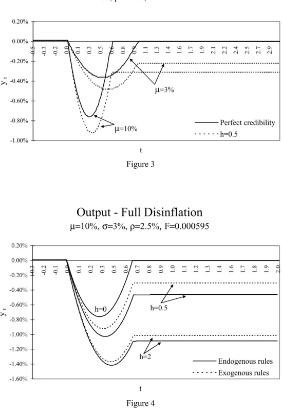
in case the stabilization is abandoned before their next pricing date. In Figure 3, on the other hand, contract lengths arefixed at the optimal level for each initial inflation rate. The
relation between inflation and the direct effect of imperfect credibility is now unclear. The
reason is that contract lengths are shorter for higher initial inflation rates and so, despite
the fact that inflation would be higher in the case of a policy reversal, the probability that
this event happens before the next pricing date is now smaller.
These results illustrate the importance of the extent of price rigidity to the assessment of the direct effect of imperfect credibility. Therefore, in all of our subsequent experiments, we fix the contract length under exogenous rules at the optimum for the initial inflationary
steady state. In our view, this is the right assumption for the experiments we analyze, which are unexpected disinflations. We start from an inflationary steady state which is
expected to last, and so it makes sense to use contract lengths which are compatible with that steady state. This allows us to properly assess the indirect effect of imperfect credibility, by appropriately taking the direct effect into account.
Figure 4 depicts the output effects of a full disinflation with our baseline calibration for
two levels of credibility (h = 0.5, and h = 2), with both endogenous and exogenous rules. The case of perfect credibility (h = 0) is presented for comparison purposes. As expected,
with imperfect credibility the recession generated is larger. It is clear that endogeneity of pricing rules reinforces this result. This happens because contract lengths increase after the disinflation begins, as firms optimally respond to lower expected inflation. With perfect
credibility, as shown in Bonomo and Carvalho (2004), in the case of full disinflation and no
strategic complementarities, the output costs of disinflation are the same with endogenous
or exogenous rules. The reason is that every firm that adjusts prices after the disinflation is
announced knows that the aggregate component of their optimal price will remain constant. Then, individual prices are set taking into account only the idiosyncratic component of the optimal price, and contract lengths have no aggregate impact. With imperfect credibility this result ceases to be true, since agents attribute some probability that the monetary authority will abandon the stabilization before their next pricing date, in which case inflation
will resume. With endogenous rules, prices are optimally set for a longer interval when compared with the exogenous rules case, which implies a higher (subjective) probability of abandonment before the next pricing date. Therefore, prices are set at higher levels and the recession is larger. This is a result of the interaction between imperfect credibility and the optimality of contract lengths.
If credibility is lower, contract lengths increase less after the disinflation is announced,
and so the differences between the endogenous and the exogenous rules cases are attenuated. On the other hand, the differences between these two cases and the perfect credibility case are amplified due to the direct effect of imperfect credibility, as can be noted in Figure 4.
In Figure 5 we explore the role of idiosyncratic uncertainty. In the case of a perfectly credible full disinflation, idiosyncratic shocks are required for optimal contract lengths to
be finite after the policy change. Otherwise, with zero inflation and no uncertainty, there
would be no reason to incur the cost to make pricing decisions.15 With imperfect credibility,
however, this is no longer the case, since the possibility of a policy reversal leads firms to
chose finite contract lengths irrespective of idiosyncratic uncertainty. The lower σ is, the
more optimal contract lengths are sensitive to inflation. So, when σ = 0 the differences between the endogenous and the exogenous rules cases are amplified, because firms choose
relatively longer contract lengths. This comparison is illustrated in Figure 5, against our benchmark value σ= 3%.
These results on the effects of different levels of credibility and idiosyncratic uncertainty illustrate important general features of the interaction between imperfect credibility and endogeneity of contract lengths, which also apply to the other results that we present. To
avoid having too many simulations, however, we chose to illustrate them only through the previous experiments.
A partial disinflation presents some qualitative differences when compared to a full disin-flation. The reason is that, with nominal rigidity in individual prices, the expected
discrep-ancy while there is no individual price adjustment only remains constant when the inflation
drift is zero. So, in contrast with the full disinflation case, in a partial disinflation a longer
contract length will induce firms to set higher prices even with full credibility. With partial
disinflation and imperfect credibility, continuing inflation and the probability of reneging
interact with the contract length and affect pricing decisions. Given the optimally chosen longer contract length,firms incorporate both the (higher) probability of abandonment and
ongoing inflation when setting their prices. As a consequence, the recession tends to be
larger.
Figure 6 shows the result of a partial disinflation under imperfect credibility for both
exogenous and endogenous rules. As expected, the endogenous rule model generates a larger recession, but also output cycles. These cycles result from gaps in the new distribution of pricing dates, which are generated by the sudden increase in contract lengths.16
4
Disin
fl
ation with learning
The results analyzed so far correspond to a situation in which the monetary authority never reneges on the announced disinflation, but nevertheless agents continue to believe that there
is always the same probability of a policy reversal. Thus, the recession continues indefinitely,
which is clearly unrealistic.
This result arises from the conjunction of two assumptions: initial beliefs that do not correspond to the true type of the monetary authority,17 and lack of updating of such beliefs
as disinflation evolves.
Discrepancies between agents’ beliefs and the actual type of the monetary authority capture the essence of the problem faced by a monetary authority that is really serious about disinflating, but has low credibility. Lack of updating of beliefs, on the other hand, is
clearly an extreme and unrealistic assumption, which we drop in this section.
We analyze how credibility evolves during disinflation, and how this interacts with optimal
price setting behavior to determine the output costs of disinflation. Initially, all agents
hold the same beliefs about the type of the monetary authority that they face. After the
16Note that those gaps also occur in the case of full disin
flation. However, they cause no output oscillation
since on averagefirms keep their prices constant.
disinflation is launched, on every pricing date firms update their beliefs about the type of
the monetary authority, taking into account whether or not disinflation has been abandoned.
Updating is done according to Bayes’ rule.
In the next subsection we present the framework with learning, and derive the optimal pricing rule. We then specialize to the case of a monetary authority who is fully committed to disinflate, but initially lacks credibility. We compare the costs of disinflation under both
endogenous and exogenous pricing rules.
4.1
Optimal pricing rule
We assume that there are two possible types for the monetary authority, characterized by the constant hazard rate for the Poisson process according to which it reneges on the promise to disinflate: h > h>0. We assume that when the disinflation policy is launched at t= 0,
agents have the same belief about the type of monetary authority they face. We denote by
π the prior probability of the monetary authority being of type h.
At any timet >0, wheneverfirms incur the pricing cost to gather and process information
and make pricing decisions, they observe whether disinflation has been abandoned and,
conditional on no abandonment, form the posterior πt, according to Bayes’ rule:18
πt ≡ Pr{h=h|Nt = 0}
= Pr{h=h, Nt= 0}
Pr{h=h, Nt= 0}+ Pr©h=h, Nt = 0ª
= πe−
ht
πe−ht+ (1−π)e−ht. (14) Now the relevant state variable for the pricing problem is augmented by the posterior belief πt, given by (14). Given the parameters h, h and the initial belief π, the posterior
is a function only of the time elapsed since disinflation was launched. While there is no
abandonment, the optimization problem of afirm on a pricing date t is given by:
Vtπ = min zt,τt
"
πtGh(zt, τt) + (1−πt)Gh(zt, τt) +
e−ρτt³F +³π
te−hτt + (1−πt)e−hτt
´
Vπ t+τt +
³
1−³πte−hτt + (1−πt)e−hτt
´´
Vµ
´ #
.
(15) We solve the above problem numerically, as described in Appendix B.
4.2
Results
We focus on the case of a monetary authority that is fully committed to disinflate (i.e., of
type h= 0) but faces a credibility problem at the time of the policy change (h >0, π <1). Figure 7 presents the path for the optimal contract length during a full disinflation. When
the disinflation begins att= 0,firms who happen to be on a pricing date choose tofix prices
for longer periods when compared to the inflationary steady-state, and therefore optimal
contract lengths jump. As the disinflation evolves, the monetary authority gains credibility
andfirms who make pricing decisions subsequently choose progressively longer contracts. In
the limit, as t → ∞, agents end up believing that the monetary authority is actually not
going to renege, and so optimal contract lengths approach their optimal zero inflation level.
The paths for output under both endogenous and exogenous pricing rules are presented in Figure 8. They share the general features of the full disinflation case without learning (Figure
4), with one noticeable exception: now, as credibility builds up, output reverts towards the steady state level. Once more, the recession is larger under endogenous pricing rules.
The differences between these results and the ones for a full disinflation without learning
hinge on the process of updating of beliefs. According with our assumptions, on pricing datesfirms update their beliefs about the type of the monetary authority they face. Because firms choose different contract lengths and are staggered in terms of their pricing dates, at
each point in time there is an endogenously determined distribution of beliefs among price-setters, which can be represented by ©πjt
ª1
j=0, where π
j t ≡ Pr
©
h=h|Ntji = 0
ª
, and tji ≤ t represents firm j0s last pricing date.
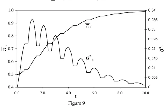
We summarize the evolution of this distribution of beliefs during disinflation by its mean
(πt ≡
R1 0 π
j
tdj) and standard deviation (σπt ≡
qR1 0
¡
πjt −πt
¢2
dj), which we present in Figure
9. When the disinflation is launched all agents hold the same belief, given by the common
prior π. As disinflation evolves, price-setters who collect information update their beliefs
upwards, and therefore the average belief increases at the same time asσπ
t starts to indicate dispersion in the corresponding distribution. This process continues for a while, with beliefs becoming more dispersed asfirms choose longer contracts and update at different times, until
a point in which the tendency reverts and beliefs start to converge, albeit non-monotonically. Meanwhile, the average belief increases steadily towards unity.
5
Conclusion
The role of credibility in monetary disinflations depends critically on the extent of price
a model in which the time period between individual price adjustments is chosen optimally ex-ante. As a result we are able to evaluate both the direct effect of credibility, for a given frequency of price adjustments, and the indirect effect, which is engendered by the optimality of price setting rules. The latter is important, as the effects of imperfect credibility and endogeneity of pricing rules interact to generate larger costs of disinflation. When the model
is augmented with learning, it generates a realistic output pattern for the disinflation process.
References
[1] Almeida, H. and M. Bonomo (2002), “Optimal State-Dependent Rules, Credibility and Inflation Inertia,”Journal of Monetary Economics 49: 1317-1336.
[2] Backus, D. and J. Driffill (1985a), “Rational Expectations and Policy Credibility Fol-lowing a Change in Regime,” Review of Economic Studies 52: 211-221.
[3] Backus, D. and J. Driffill (1985b), “Inflation and Reputation,” American Economic Review 75: 530-538.
[4] Ball, L. (1995), “Disinflation with Imperfect Credibility,” Journal of Monetary Eco-nomics 35: 5-23.
[5] Ball, L. and G. Mankiw (1994), “Asymmetric Price Adjustment and Economic Fluctu-ations,” Economic Journal 104: 247-261.
[6] Ball, L., N. G. Mankiw and D. Romer (1988), “The New Keynesian Economics and the Output-Inflation Trade-off,” Brookings Papers on Economic Activity 1: 1-65.
[7] Ball, L. and D. Romer (1990), “Real Rigidities and the Non-Neutrality of Money,” Review of Economic Studies 57: 183-203.
[8] Bils, M. and P. Klenow (2004), “Some Evidence on the Importance of Sticky Prices,” Journal of Political Economy 112: 947-985.
[9] Blinder, A., E. Canetti, D. Lebow, and J. Rudd (1998), Asking about Prices: A New Approach to Understanding Price Stickiness, Russel Sage Foundation.
[10] Bonomo, M. and C. Carvalho (2004), “Endogenous Time-Dependent Rules and Inflation
Inertia,” Journal of Money, Credit and Banking 36: 1015-1041.
[11] Caplin, A. and J. Leahy (1991), “State-Dependent Pricing and the Dynamics of Money and Output,”Quarterly Journal of Economics 106: 683-708.
[12] _______________ (1997) “Aggregation and Optimization with State-Dependent Pricing,” Econometrica 65: 601-625.
[13] Caplin, A. and D. Spulber (1987), “Menu Costs and the Neutrality of Money,”Quarterly Journal of Economics 102: 703-726.
[15] Conlon, J. and C. Liu (1997), “Can More Frequent Price Changes Lead to Price Inertia? Nonneutralities in a State-Dependent Pricing Context,”International Economic Review 38: 893-914.
[16] Dhyne, E., L. Álvarez, H. Le Bihan, G. Veronese, D. Dias, J. Hoffman, N. Jonker, P. Lünnemann, F. Rumler and J. Vilmunen (2006), “Price Changes in the Euro Area and the United States: Some Facts from Individual Consumer Price Data,” Journal of Economic Perspectives 20: 171-192.
[17] Erceg, C. and A. Levin (2003), “Imperfect Credibility and Inflation Persistence,” Jour-nal of Monetary Economics 50: 915-944.
[18] Ferreira, S. (1994), “Inflação, Regras de Reajuste e Busca Sequencial: Uma Abordagem
sob a Ótica da Dispersão de Preços Relativos,” M.A. Dissertation, PUC-Rio.
[19] Gagnon, E. (2006), “Price Setting During Low and High Inflation: Evidence from
Mex-ico,” mimeo, Federal Reserve Board.
[20] Gertler, M. and J. Leahy (2006), “A Phillips Curve with an Ss Foundation,” NBER Working Paper #11971.
[21] Golosov, M. and R. Lucas (2007),“Menu Costs and Phillips Curves,”Journal of Political Economy 115: 171-199.
[22] Huang, K. and C. Liu (2002), “Staggered Price-Setting, Staggered Wage-Setting, and Business Cycle Persistence,” Journal of Monetary Economics 49: 405-433.
[23] Konieczny, J. and A. Skrzypacz (2005a), “Inflation and Price Setting in a Natural
Experiment,” Journal of Monetary Economics 52: 621-632.
[24] Lach, S. and D. Tsiddon (1992), “The Behavior of Prices and Inflation: An Empirical
Analysis of Disaggregated Price Data,” Journal of Political Economy 100: 349-389.
[25] Mankiw, G., and R. Reis (2002), “Sticky Information Versus Sticky Prices: A Proposal to Replace the New Keynesian Phillips Curve,” Quarterly Journal of Economics 117: 1295-1328.
[26] Nakamura, E. and J. Steinsson (2007), “Five Facts About Prices: A Reevaluation of Menu Cost Models,” mimeo, Harvard University.
[28] Reis, R. (2006), “Inattentive Producers,”Review of Economic Studies 73: 793-821.
[29] Sargent, T. (1983), “Stopping Moderate Inflations: The Methods of Poincare and
Thatcher,” in: Dornbusch, R. and M. Simonsen (eds.), Inflation, Debt and Indexation, MIT Press, Cambridge, MA.
[30] Siu, H. (2007), “Time Consistent Monetary Policy with Endogenous Price Rigidity,” forthcoming in the Journal of Economic Theory.
[31] Taylor, J. (1979), “Staggered Wage Setting in a Macro Model,” American Economic Review 69: 108-113.
[32] Taylor, J. (1980), “Aggregate Dynamics and Staggered Contracts,”Journal of Political Economy 88: 1-23.
[33] Westelius, N. (2005), “Discretionary Monetary Policy and Inflation Persistence,” Jour-nal of Monetary Economics 52: 477-496.
[34] Woodford, M. (2003),Interest and Prices: Foundations of a Theory of Monetary Policy, Princeton University Press.
Appendix A
Here we derive the frictionless optimal price in a general equilibrium framework with industry-specific shocks.
A representative consumer maximizes the following utility function:19
E0
½Z ∞
0
e−ρ(t−t0) ∙
u(Ct)−
Z 1
0
v(hjt)dj
¸
dt
¾
where
Ct≡
∙Z 1
0
Cjt
θ−1
θ dj
¸ θ θ−1
,
with θ >1, and Pt is defined by
Pt≡
∙Z 1
0
Pjt1−θdj
¸ 1 1−θ
, (16)
subject to the corresponding budget constraints:
Bt =B0+ Z t
0 µZ 1
0
Wjshjsdj
¶ ds− Z t 0 µZ 1 0
PjsCjsdj
ds+
Z t
0
Tsds+
Z t
0
ΛsdXs+
Z t
0
ΛsdDs, for t≥0,
where Cjs is the consumption of good j, Pjs is its price, hjs is the supply of labor of type j, which receives wageWjs, Btis totalfinancial wealth,Tsdenotes total net transfers, including any lump-sumflow transfer from the government, and profits received from thefirms, which
are owned by the representative consumer. Xs is the vector of prices of traded assets,Ds is the corresponding vector of cumulative dividend processes, and Λs is the trading strategy, which we assume satisfies conditions that preclude Ponzi schemes.
In this setting, the demand for an individual product has the following familiar relation with aggregate demand:
Cjt =
µ
Pjt
Pt
¶−θ
Ct. (17)
Firms are divided into industries that have specific and competitive labor markets. All firms in an industry change prices at the same time, and are subject to common productivity
shocks. Each firm uses labor of the appropriate type to produce a specific variety of the
consumption good.
Each firm in industryj hires type-j labor to produce variety j of the consumption good according to the following production function:
Yjt =Ajtf(hjt),
where Ajt is the industry productivity process. It is decomposed as:
Ajt = exp{εjt}= exp
©
εt+ξjt
ª
,
where εt is the aggregate productivity component given by εt ≡ R01εjtdj, and ξjt is an industry-specific component.20 We assume that industry-specific components have the same
law of motion for all industries, and are mutually independent.
Under flexible prices, each producer chooses its supply to maximize profits. The
corre-sponding first order condition is:21
µ Yt Yjt ¶1 θ = θ
θ−1s(Yjt, Yt, Ajt), (18) where we have used the equilibrium conditionYt=Ct, ands(Yjt, Yt, Ajt)is the real marginal cost of producing Yjt:
s(Yjt, Yt, Ajt) =
vh(f−1(Yjt/Ajt))
uc(Yt)Ajt
Ψ µ Yjt Ajt ¶ , where
Ψ(Y)≡ 1
f0(f−1(Y)).
In this economy a flexible price equilibrium is characterized by a valid equation (18) for each j andYt given by:22
Yt ≡
∙Z 1
0
Y θ−
1
θ
jt dj
¸ θ θ−1
. (19)
We define the level of natural output Yn
t as the aggregate output level corresponding to the flexible price equilibrium. This is similar to the standard concept in the literature (e.g.
20Note that our decomposition and the definition of ε
timply thatξjt’s have zero mean in the cross-section of industries.
21Recall that producers takes wages as given when maximizing profits, because industry-specific labor markets are competitive.
22Equations (18) and (19) de
fine implicitly a functionΘ:³{Ykt}k6=j , Ajt ´
→Yjt. For a given realization Ajt, define Θjt
³
{Ykt}k6=j
´
≡ Θ³{Ykt}k6=j, Ajt ´
. For given realizations Ajt for all j, an equilibrium is a
Woodford, 2003, chapter 3). However, notice that here each individual output level in general differs from Yn
t due to the existence of industry-specific shocks.
Proceeding analogously as in Woodford (2003), we define the steady state level of
pro-duction,Y, as the output level in the symmetricflexible price equilibrium when εjt = 0 for allj. So, it satisfies:
1 = θ
θ−1s
¡
Y , Y ,1¢.
In order to obtain a more explicit characterization of the flexible price equilibrium we
loglinearize both sides of equation (18) around steady state levels and rearrange to get:
b
yjt =
1−θλ−1
1 +θω ybt+
(1 +ω)θ
1 +θω εjt, (20)
where byjt ≡log
³Y
jt
Y
´
,ybt≡log¡YYt¢, ω≡
∂logs(Y ,Y ,0)
∂logyi , and λ
−1
≡ −∂log∂loguc(YY).
Loglinearizing (19), and using (20), we obtain a relation between the natural output rate and the aggregate shock:
b
yn t =
1 +ω
ω+λ−1εt, (21)
where bytn≡log
³Yn t
Y
´
.
In order to derive a relation between the individual optimal price and the output gap, we first loglinearize the demand function:23
b
yjt =ybt−θ(pjt−pt), (22) where pjt ≡logPjt, and pt ≡logPt.
Then, we substitute (22) into (20) to get:
pjt−pt=
ω+λ−1
1 +θω byt−
1 +ω
1 +θωεjt.
Finally, we decompose εjt into its aggregate and industry-specific components and use (21) to replace εt, obtaining:
pjt−pt=γ(yt−ytn) +ejt, (23) where yt ≡logYt,ytn≡logYtn, ejt ≡ −1+1+θωω ξjt, and γ ≡ ω+λ
−1 1+θω >0.
Since our focus is on the supply side of the model, we take (log) nominal aggregate demand {Yt}t=0 to be an exogenous process. Substituting yt ≡ Yt−pt into (23) we arrive
at the expression for the frictionless optimal price presented in the main text:
pjt = (1−γ)pt+γ(Yt−ytn) +ejt. (24)
Appendix B
Here we present the solution method for (15). The corresponding first order conditions
are:
zt∗ = ρ 1−e−ρτ∗
t
Z τ∗
t
0 "
µ0s+ (µ−µ0)
Ã
s−
Ã
πt
1−e−hs
h + (1−πt)
Ã
1−e−hs h
!!!#
e−ρsds; (25)
(zt∗−µ0τ∗ t)
2
+σ2τ∗ t +
³
πthe−hτ
∗
t + (1−π
t)he−hτ
∗
t
´ ³
Vµ−Vtπ+τ∗
t
´
+ (26)
³
πte−hτ
∗
t + (1−π
t)e−hτ
∗
t
´∂Vtπ+τ∗
t
∂t −ρ
³
F +Vµ+
³
πte−hτ
∗
t + (1−π
t)e−hτ
∗
t
´ ³
Vtπ+τ∗
t −Vµ
´´
+
Z τ∗
t
0
((µ0−µ) (τ∗t −r))2³πthe−hr+ (1−πt)he−hr
´
dr+
2 (µ0−µ) (z∗t −µ0τ∗t)
Z τ∗
t
0
(τ∗t −r)³πthe−hr+ (1−πt)he−hr
´
dr = 0.
Equations (25), (26), and (15) characterizezt∗,τ∗t andVπ t+τ∗
t. To solve this set of equations,
wefirst pickT large enough, such that, fort > T,Vπ
t can be taken as approximately constant. This is justified: conditional on no abandonment, the probability that the monetary authority
is of type h keeps increasing, and the problem becomes more and more similar to the one analyzed in section (2.3), withh =h. Formally, lim
t→∞πt = 1,
24 which implies that lim
t→∞V π t+τ∗
t =
Vh. So, we solve the set of equations moving backwards in time. For eachtwefindz∗
t,τ∗t and use them to computeVπ
t , which will then be used tofindz∗,τ∗at earlier times. Alternatively, to avoid numerical derivatives, one can use (25), and (15) tofindτ∗
t with a grid search, instead of using (26). This is the method we adopted.
24Just rewriteπ
tas 1
1+(1−ππ)e−(h−h)t
Obs: Contract lengths are fixed at the level corresponding to the optimum for µ=3%.
Figure 1
Figure 2
Optimal Contract Length - Full Disinflation
σ=3%, ρ=2.5%,F=0.000595
0.2 0.3 0.4 0.5 0.6 0.7 0.8 0.9 1 1.1 1.2
0.0 1.0 2.0 3.0 4.0 5.0 6.0 7.0 8.0 9.0 10.0
τ
∗
h
µ=10%
µ=20%
Direct Effect - Arbitrary Contract Lengths
Different Initial Inflation Rates - Full Disinflation
σ=3%,ρ=2.5%, F=0.000595
-1.80% -1.60% -1.40% -1.20% -1.00% -0.80% -0.60% -0.40% -0.20% 0.00% 0.20%
-0
.5
-0
.3
-0
.2 0.0 0.1 0.3 0.5 0.6 0.8 0.9 1.1 1.3 1.4 1.6 1.7 1.9 2.1 2.2 2.4 2.5 2.7 2.9
t
y t
Perfect credibility h=0.5
µ=3%
Figure 4 Figure 3
Output - Full Disinflation
µ=10%, σ=3%,ρ=2.5%, F=0.000595
-1.60% -1.40% -1.20% -1.00% -0.80% -0.60% -0.40% -0.20% 0.00% 0.20%
-0
.3
-0
.2
-0
.1 0.0 0.1 0.2 0.3 0.5 0.6 0.7 0.8 0.9 1.0 1.1 1.2 1.3 1.4 1.6 1.7 1.8 1.9 2.0
t
y t
Endogenous rules Exogenous rules
h=0 h=0.5
h=2
Direct Effect - Optimal Contract Lengths
Different Initial Inflation Rates - Full Disinflation
σ=3%,ρ=2.5%, F=0.000595
-1.00% -0.80% -0.60% -0.40% -0.20% 0.00% 0.20%
-0
.5
-0
.3
-0
.2 0.0 0.1 0.3 0.5 0.6 0.8 0.9 1.1 1.3 1.4 1.6 1.7 1.9 2.1 2.2 2.4 2.5 2.7 2.9
t
y t
Perfect credibility h=0.5
µ=3%
Figure 5
Figure 6
Output - Partial Disinflation
µ=10%, µ'=2%, h=0.5, σ=3%, ρ=2.5%, F=0.000595
-1.00% -0.80% -0.60% -0.40% -0.20% 0.00% 0.20%
-0
.3
2
-0
.1
5
0.03 0.20 0.38 0.55 0.72 0.90 1.07 1.25 1.42 1.59 1.77 1.94
y t
Endogenous rules
Exogenous rules
t
Output - Full Disinflation
µ=10%, h=0.5,ρ=2.5%, F=0.000595
-1.25% -1.05% -0.85% -0.65% -0.45% -0.25% -0.05% 0.15%
-0
.3
-0
.2
-0
.1 0.0 0.1 0.2 0.3 0.5 0.6 0.7 0.8 0.9 1.0 1.1 1.2 1.3 1.4 1.6 1.7 1.8 1.9 2.0
t
y t
Endogenous rules Exogenous rules h=0
σ=3%
Figure 7
Figure 8
Optimal Contract Length with Learning
π=0.5, h=0.5, h=0, µ=10%, σ=3%, ρ=2.5%, F=0.000595
0.40 0.50 0.60 0.70 0.80 0.90 1.00 1.10 1.20
-5.0 0.0 5.0 10.0 15.0 20.0
τ
tt
Output - Disinflation with Learning
π=0.5, h=0.5, h=0, µ=10%, σ=3%, ρ=2.5%, F=0.000595
-1.00% -0.80% -0.60% -0.40% -0.20% 0.00% 0.20%
-1.0 0.0 1.0 2.0 3.0 4.0 5.0
y t
t
Figure 9
Evolution of Beliefs
π=0.5, h=0.5, h=0, µ=10%, σ=3%, ρ=2.5%, F=0.000595
0.4 0.5 0.6 0.7 0.8 0.9 1.0
0.0 2.0 4.0 6.0 8.0 10.0
π
t
0 0.005 0.01 0.015 0.02 0.025 0.03 0.035 0.04
σ
π
t
t