Pesqui. Oper. vol.35 número1

doi: 10.1590/0101-7438.2015.035.01.0165

A BIVARIATE GENERALIZED EXPONENTIAL DISTRIBUTION DERIVED FROM COPULA FUNCTIONS IN THE PRESENCE

OF CENSORED DATA AND COVARIATES

Jorge Alberto Achcar

_{, Fernando Antˆonio Moala}

_,

Mario Hissamitsu Tarumoto

and Leandro Fernandes Coladello

Received November 4, 2012 / Accepted April 11, 2014

ABSTRACT.In this paper, we introduce a Bayesian analysis for a bivariate generalized exponential dis-tribution in the presence of censored data and covariates derived from Copula functions. The generalized exponential distribution could be a good alternative to analyze lifetime data in comparison to usual existing parametric lifetime distributions as Weibull or Gamma distributions. We have being using standard exist-ing MCMC (Markov Chain Monte Carlo) methods to simulate samples for the joint posterior of interest. Two examples are introduced to illustrate the proposed methodology: an example with simulated bivariate lifetime data and an example with a real lifetime data set.

Keywords: Bivariate generalized exponential distribution, copula function, Bayesian analysis, censored data, covariates.

1 INTRODUCTION

In medical, engineering or other lifetime data applications, we could have more than one lifetime associated to each unit. A special situation is the presence of two lifetimesT1andT2associated to each unit. In this situation, we could consider some existing bivariate lifetime distribution that has been introduced in the literature (see for example, Gumbel, 1960; Freund, 1961; Marshall & Olkin, 1967; Downton, 1972; Block & Basu, 1974; Sarkar, 1987; Hawkes, 1988).

Usually these bivariate lifetime distributions generalize some popular existing univariate lifetime distributions as exponential, Weibull, Gamma or a log-normal distribution (see for example, Lawless, 1982).

*Corresponding author.

1Departamento de Matem´atica, Estat´ıstica e Computac¸˜ao, UNESP, Universidade Estadual Paulista, Presidente Prudente, SP, Brazil. E-mail: [email protected]

Other parametrical lifetime distributions could be generalized for the bivariate case. One of these models is given by the generalized exponential distribution (see for example, Gupta & Kundu, 1999; Raqab & Ahsanullah, 2001; Raqab, 2002; Zheng, 2002; Gupta & Kundu, 2007; Sarhan, 2007). Kundu & Gupta (2009) introduced a singular bivariate Generalized Exponential (BVGE) distribution to analyze lifetime data.

An alternative and flexible way to derive different bivariate lifetime distributions could be given by copula functions (see, for example, Trived & Zimmer, 2005a,b; Nelsen, 2006). There are several copula functions in the literature for construction of multivariate liftetime distributions where the most used are Farlie-Gumbel-Morgensten (Morgensten, 1956), and the Archimedean copulas as Clayton (1978), Gumbel (1960) and Frank (1979).

Recently, new copulas have been proposed as the class of Archimedean copulas ind-dimension given in McNeil & Neslehov´a (2009). McNeil & Neslehov´a (2010) also generalise the Archi-medean copulas to obtain the Liouville copula. Marshall-Olkin Copulas (see Li, 2012) and the Generalized Farlie-Gumbel-Morgenstern copula (Bekrizadeh et al., 2012) are other examples.

Achcar & Santos (2010) construct bivariate Weibull distributions suitable for survival analysis by using different copula functions. The bivariate Birnbaum-Saunders distribution proposed by Kundu et al. (2010) show that it can be obtained as a Gaussian copula. More recently, Kundu introduced the bivariate Sinh-normal distribution, which can be obtained as a bivariate Gaussian copula.

Kundu & Gupta (2011) also derived an absolute continuous bivariate Generalized Exponential distribution based on the Clayton copula.

In this paper, we introduce other bivariate generalized exponential distributions derived from the Farlie-Gumbel-Morgensten to analyze lifetime data. We also investigate the performance of this new distribution.

Inferences for these different versions of bivariate lifetime models could present some difficul-ties using standard classical inference methods, especially in the presence of censored data and covariates, a usual situation in applications.

In this way, we consider the use of Bayesian methods where the samples for the joint posterior distribution of interest are simulated using MCMC (Markov Chain Monte Carlo) methods as the popular Gibbs sampling algorithm (see for example, Gelfand & Smith, 1990; or Casela & George, 1992) or the Metropolis-Hastings algorithm (see for example, Chib & Greenberg, 1995).

2 COPULA FUNCTIONS

Copula functions can be used to link marginal distributions with a joint distribution. For specified univariate marginal distribution functionsF1(t1),F2(t2), . . . ,Fm(tm), the function,

C(F1(t1),F2(t2), . . . ,Fm(tm))=F(t1,t2, . . . ,tm) (1)

which is defined using a copula functionC, results in a multivariate distribution function with univariate marginal distributions specified asF1(t1),F2(t2), . . . ,Fm(tm), (see for example, Frees (1998) or Nelsen (1999)).

It is important to point out that any multivariate distribution functionFcan be written in the form of a copula function (Sklar, 1959); that is, ifF(t1,t2, . . . ,tm)is a joint multivariate distribution function with univariate marginal distribution functions F1(t1),F2(t2), . . . ,Fm(tm), thus there exists a copula functionC(U1,U2, . . . ,Um)such that (1) occurs.

If everyFi is continuous, thenCis unique.

In the bivariate cases, letT1andT2be two random variables with continuous distribution func-tionsF1andF2.

The probability integral transform can be applied separately to the two random variables to de-fineU = F1(t1)andV = F2(t2), whereU andV have uniform(0,1)distributions, but are usually dependent ifT1andT2are dependent (T1andT2independent, implies thatU andV are independent).

Specifying dependence between T1 andT2 is the same as specifying dependence between U andV.

WithU andV uniform random variables, the problem reduces to specifying a bivariate distribu-tion between two uniforms, that is, a copula.

3 GENERALIZED EXPONENTIAL DISTRIBUTION

A generalized exponential distribution (see Gupta & Kundu, 1999) can be a good alternative to the usual Gamma and Weibull distributions commonly used to analyse lifetime data (see also, Raqab & Ahsanullah, 2001; Raqab, 2002; Zheng, 2002; Gupta & Kundu, 2007, 2008; Sarhan, 2007).

The generalized exponential distribution with two parameters has density given by,

f(t;α, λ)=αλ[1−exp(−λt)]α−1exp(−λt), (2)

wheret >0,α >0, andλ >0, are respectively, shape and scale parameters.

The survival and hazard functions associated to (2), are given, respectively, by,

S(t; α, λ)=P{T >t} =1−

1−exp(−λt) α

. (3)

and

h(t;α, λ)= f(t;α,λ) S(t;α,λ) =

αλ[1−exp(−λt)]α−1exp(−λt)

1−

1−exp(−λt)

α . (4)

Observe that the hazard functionh(t;α, λ)is increasing from 0 toλifα >1; decreasing ifα <1 and constant ifα=1.

This behavior of the hazard function is similar to the behavior of the hazard function of the gamma distribution.

The moment generation function for a random variableT with a generalized exponential distri-bution with density (2) is given (see Gupta & Kundu, 2008) by,

M(s)=E[esT] = Ŵ(α+1)Ŵ(1−s/λ)

Ŵ(α+1−s/λ) , (5)

fors< λ;Ŵ(x)is the gamma function.

From (5), we get the moments of interest. The mean and variance ofT are given, respectively, by,

E(T)= 1 λ

ψ (α+1)−ψ (1) and

var(T)= 1 λ2

ψ′(1)−ψ′(α+1),

(6)

whereψ (·)is the digamma function given by

ψ (x)= d

d xlogŴ(x)=

Ŵ′(x) Ŵ(x).

4 A BIVARIATE GENERALIZED EXPONENTIAL DISTRIBUTION DERIVED

FROM THE FARLIE-GUMBEL-MORGENSTERN COPULA

Different copula functions introduced in the literature could be used to obtain a bivariate gener-alized exponential distribution.

A special case is given by the Farlie-Gumbel-Morgensten Copula (see Morgensten, 1956) given by,

C(u, v)= [1−eln(1−u)][1−eln(1−v)]

1+θexpln(1−u)+ln(1−v)

(7)

where−1≤θ ≤1,u =F1(t1)(marginal distribution for the random variableT1) andv=F2(t2)

Observe thatθis a parameter associated to the dependence between the random variablesT1and T2and related to the Spearman’s rank correlationρS(T1,T2)(“Spearman’s rho”) and Kendall’s rank correlationρτ(T1,T2)(“Kendall’s tau”) by the relations,

ρS(T1,T2)=12

1

0

C(u, v)−uv

dudv and

ρτ(T1,T2)=4

1

0

1

0

C(u, v)dC(u, v)−1.

(8)

From (7), we getρS(T1,T2)=θ /3 andρτ(T1,T2)=2θ /9 (see for example, Nelsen, 1999).

From (8), we could use the information of experts to directly elicit a prior distribution for the correlation (a value between−1 and 1) betweenT1andT2; another possibility is to use empir-ical Bayesian methods to choose a prior distribution for the dependence parameterθ using the relations given by (8). Some authors introduce different methods for eliciting a prior distribution for the correlation (see for example, Clemen, Fischer & Winkler, 2000).

Let us assume the marginal generalized exponential distributions (see (2)), given by,

u=F1(t1)=P{T1≤t1} =

1−exp(−λ1t1)

α1

and

v=F2(t2)= P{T2≤t2} =

1−exp(−λ2t2) α2

(9)

From (7), the joint distribution function forT1andT2is given by,

F(t1,t2|, λ1, λ2, α1, α2, θ )=(1−e−λ1t1)α1(1−e−λ2t2)α2

×1+θ1−(1−e−λ1t1₎α1_1−(1−e−λ2t2₎α2

(10)

wheret1>0 andt2>0.

The joint density function forT1andT2is given by,

f(t1,t2|λ1, λ2, α1, α2, θ )=

∂2F(t1,t2)

∂t1∂t2

(11)

That is, from (11), we have,

f(t1, t2|λ1, λ2, α1, α2, θ )= f1(t1)f2(t2)+θf1(t1)f2(t2)

1−2F1(t1)

1−2F2(t2)

(12)

where f1(t1)and f2(t2)are the marginal densities for T1andT2 with parameters(α1, λ1)and

(α2, λ2), respectively (see (2)), andF1(t1)andF2(t2)are given by (9).

x 1 2 3 4 y 0.5 1.0 1.52.0 0.1 0.2 0.3 (a) _(b)

0 1 2 3 4

0.0 0.5 1.0 1.5 2.0 2.5 theta=0.5 (c)

0 1 2 3 4

0.0 0.5 1.0 1.5 2.0 2.5 theta=0.01 (d)

0 1 2 3 4

0.0 0.5 1.0 1.5 2.0 2.5 theta=0.9 (e)

0 1 2 3 4

0.0 0.5 1.0 1.5 2.0 2.5 theta=−0.5 (f)

0 1 2 3 4

0.0 0.5 1.0 1.5 2.0 2.5 theta=−0.8

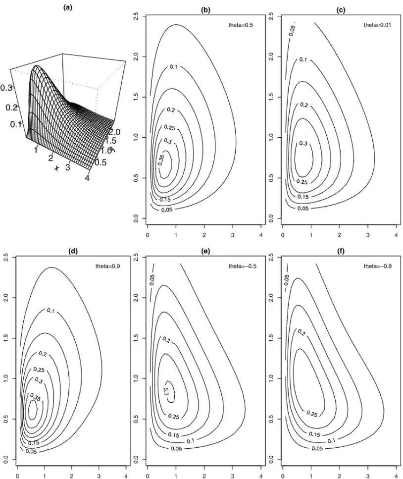
Figure 1– Contour plots of bivariate density with generalized exponential marginal densities.

Also observe that the joint bivariate survival function for the lifetimesT1andT2is given by, S(t1,t2)= P{T1>t1,T2>t2} =1−F1(t1)−F2(t2)+F(t1,t2), (13)

whereF1(t1)andF2(t2)are given by (9) andF(t1,t2)is given by (10). That is, S(t1,t2)=1−(1−e−λ1t1)α1 −(1−e−λ2t2)α2 +(1−e−λ1t1)α1(1−e−λ2t2)α2

×

1+θ

1−(1−e−λ1t1₎α1_1−(1−e−λ2t2₎α2

(14)

5 A BAYESIAN ANALYSIS IN THE PRESENCE OF CENSORED DATA

Suppose eitherT1orT2can be censored and that censoring is independent of the lifetimes. Let us subdivide thenobservations into four classes:

C1: botht1i andt2i are observed lifetimes,i=1, . . . ,n;

C2:t1iis a lifetime andt2i is a censoring time (that is, we only know thatT2i ≥t2i); C3:t1iis a censoring time andt2iis a lifetime;

C4: botht1i andt2i are censoring times.

The likelihood function for a continuous model (see for example, Lawless, 1982, page 479) is given by,

L = i∈C1

f(t1i,t2i) i∈C2

−∂S(t1i,t2i) ∂t1i

i∈C3

−∂S(t1i,t2i) ∂t2i

i∈C4

S(t1i,t2i) (15)

where f(t1i,t2i)is the joint probability density function forT1i andT2i;S(t1i,t2i)is the joint survival function;∂S(t1i,t2i)

∂t1i and

∂S(t1i,t2i)

∂t2i are the partial derivatives ofS(t1i,t2i)with respect to

t1iandt2i, respectively.

Let us define the indicator variablesδ1i andδ2i, by,

δj i =

1 iftj iis an observed lifetime 0 iftj iis a censored observation

(16)

forj =1,2;i =1, . . .n, wherenis the number of observations. In this way, we rewrite the likelihood function (15) as,

L= n

i=1

f(t1i,t2i) δ1iδ2i n

i=1

−∂S(t1i,t2i) ∂t1i

δ1i(1−δ2i)

× n

i=1

−∂S(t1i,t2i) ∂t2i

(1−δ1i)δ2i n

i=1

S(t1i,t2i)

(1−δ1i)(1−δ2i)

(17)

Observe that if we do not have censored data, the likelihood function (17) reduces to,

L = n

i=1

In (17), we replace S(t1i,t2i) by (14), f(t1i,t2i)by (12), and F1(t1i)and F2(t2i)are given by (9), that is,

f(t1i,t2i|λ1, λ2, α1, α2, θ )=α1α2λ1λ2(1−e−λ1t1i)α1−1(1−e−λ2t2i)α2−1

×exp(−λ1t1i−λ2t2i)

1+θ

1−2(1−e−λ1t1i₎α1_1−2(1−e−λ2t2i₎α2

(19)

The first derivatives ofS(t1i,t2i)with respect tot1iandt2i are given by,

−∂S(t1i,t2i) ∂t1i

= f1(t1i)

1−F2(t2i)

1+θ

1−F2(t2i)

1−2F1(t1i)

and

−∂S(t1i,t2i) ∂t2i

= f2(t2i)

1−F1(t1i)

1+θ

1−F1(t1i)

1−2F2(t2i)

(20)

that is,

−∂S(t1i,t2i) ∂t1i

=α1λ1(1−e−λ1t1i)α1−1e−λ1t1i

1−(1−e−λ2t2i₎α2

×

1+θ

1−(1−e−λ2t2i₎α2

1−2(1−e−λ1t1i₎α1

and

−∂S(t1i,t2i) ∂t2i

=α2λ2(1−e−λ2t2i)α2−1e−λ2t2i

1−(1−e−λ1t1i₎α1

×

1+θ

1−(1−e−λ1t1i₎α1

1−2(1−e−λ2t2i₎α2

(21)

For a Bayesian analysis, let us assume the following prior distribution forλ1, λ2, α1, α2andθ:

λj ∼U[ajbj] αj ∼U[cjdj] θ ∼U[−1,1]

(22)

for j=1,2;U[a,b]denotes an uniform distribution in the interval(a,b);aj, bj,cj anddjare known hyperparameters. We further assume prior independence among the parameters.

Other prior distributions also could be considered, as gamma priors forαj andλj, j=1,2. The joint posterior distribution forv=(λ1, λ2, α1, α2, θ )′is given by,

π(v|t_{)∝π(v)L(v|}t_{) (23)}

whereπ(v)is the joint prior distribution forv;L(v|t_{)is the likelihood function (17) and}t ₌

(t_{1, . . . ,}t_n), t_{i =(t1i,t2i),i=1, . . . ,nis a vector of observed lifetime data.}

To get the posterior summaries of interest, we simulate samples for the joint posterior distribu-tion (23) using MCMC methods.

π(α2|λ1,λ2,α1,θ ,t)andπ(θ|λ1,λ2,α1,α2,t)using the Gibbs sampling algorithm or the Metropolis-Hastings algorithm, when the conditional distributions are not identified as known distributions that are easy to simulate.

Considering the presence of a vector X =(X1,X2, . . . , Xp)′ of covariates associated to each bivariate lifetimeT1andT2, let us consider the following regression model:

λ1i =γ1exp(β ′ 1xi) λ2i =γ2exp(β

′ 2xi)

(24)

whereβ_j =(βj1, βj2, . . . , βj p)′is the regression parameter vector, j =1,2, associated to the covariate vectorx_{i =(x1i,x2i, . . . ,xpi)}′_{,i=1,2, . . . ,n.}

We also assume the presence of censored observations.

For a Bayesian analysis, we assume the following prior distributions forγj, αj, βj k andθ:

αj ∼U[ajbj] γj ∼U[cjdj] θ∼U[−1,1] βj k ∼N(0,g2)

(25)

for j =1,2;k =1, . . . ,pand aj,bj,cj,dj andg are known hyperparameters andN(0,g2) denotes a normal distribution with mean zero and varianceg2. We further assume prior indepen-dence among the parameters.

6 APPLICATIONS

6.1 Simulated data sets

As a first application, let us consider four simulated data sets from the bivariate generalized exponential distribution (10) in the presence of censored data with sample sizesn=10 (d1=10, d2=9);n=20 (d1=18,d2=20);n=30 (d1=27,d2=30) andn=50 (d1=44,d2=47) whered1is the number of uncensored lifetimest1i andd2is the number of uncensored lifetimes

t2i, i = 1,2, . . . ,n, and the following values for the parameters of the model: λ1 = 0.001;

λ2=0.005;α1=1;α2=0.5 andθ=0.5.

We assume a reparametrization forλ1andλ2given byγ1∗ = log(λ1)andγ2∗ =log(λ2)to get better convergence for the Gibbs sampling algorithm using the software Winbugs (Spiegelhalter et al., 2003) which only requires the specification of the joint distribution for the data and prior distributions for the parameters. For all considered sample sizes, we assume the following prior distributions:

γ₁∗∼U(−10,0), γ∗

2 ∼U(−10,0), α1∼U(0,3), α2∼U(0,2) and θ∼U(0,1).

informative prior distributions. Thus, a sensitivity analysis was performed to determine a final specification of the parameters. Here we present only the best result we obtained for these priors.

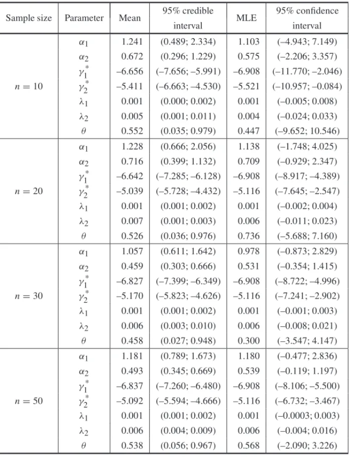
In Table 1, we have the posterior summaries of interest obtained from a final simulated Gibbs sample of size 2000 of the joint posterior distribution for the parameters of the model after discarding the first 5000 Gibbs samples to eliminate the effect of the initial values for the Gibbs sampling algorithm. In Table 1, we also have the maximum likelihood estimates (MLE) and the 95% confidence intervals based on the asymptotical normality of the MLE.

Table 1– Posterior summaries (simulated data sets) and MLE estimates.

Sample size Parameter Mean 95% credible MLE 95% confidence

interval interval

α1 1.241 (0.489; 2.334) 1.103 (–4.943; 7.149)

α2 0.672 (0.296; 1.229) 0.575 (–2.206; 3.357)

γ₁* –6.656 (–7.656; –5.991) –6.908 (–11.770; –2.046) n=10 γ₂* –5.411 (–6.663; –4.530) –5.521 (–10.957; –0.084)

λ1 0.001 (0.000; 0.002) 0.001 (–0.005; 0.008)

λ2 0.005 (0.001; 0.011) 0.004 (–0.024; 0.033)

θ 0.552 (0.035; 0.979) 0.447 (–9.652; 10.546)

α1 1.228 (0.666; 2.056) 1.138 (–1.748; 4.025)

α2 0.716 (0.399; 1.132) 0.709 (–0.929; 2.347)

γ₁* –6.642 (–7.285; –6.128) –6.908 (–8.917; –4.389) n=20 γ₂* –5.039 (–5.728; –4.432) –5.116 (–7.645; –2.547)

λ₁ 0.001 (0.001; 0.002) 0.001 (–0.002; 0.004)

λ2 0.007 (0.001; 0.003) 0.006 (–0.011; 0.023)

θ 0.526 (0.036; 0.976) 0.736 (–5.688; 7.160)

α₁ 1.057 (0.611; 1.642) 0.978 (–0.873; 2.829)

α2 0.459 (0.303; 0.666) 0.531 (–0.354; 1.415)

γ₁* –6.827 (–7.399; –6.349) –6.908 (–8.722; –4.996) n=30 γ₂* –5.170 (–5.823; –4.626) –5.116 (–7.241; –2.902)

λ1 0.001 (0.001; 0.002) 0.001 (–0.001; 0.003)

λ₂ 0.006 (0.003; 0.010) 0.006 (–0.008; 0.021)

θ 0.458 (0.027; 0.948) 0.300 (–3.547; 4.147)

α1 1.181 (0.789; 1.673) 1.180 (–0.477; 2.836)

α₂ 0.493 (0.345; 0.669) 0.539 (–0.119; 1.197)

γ₁* –6.837 (–7.260; –6.480) –6.908 (–8.106; –5.500) n=50 γ₂* –5.092 (–5.594; –4.666) –5.116 (–6.732; –3.467)

λ1 0.001 (0.001; 0.002) 0.001 (–0.0003; 0.003)

λ2 0.006 (0.004; 0.009) 0.006 (–0.004; 0.016)

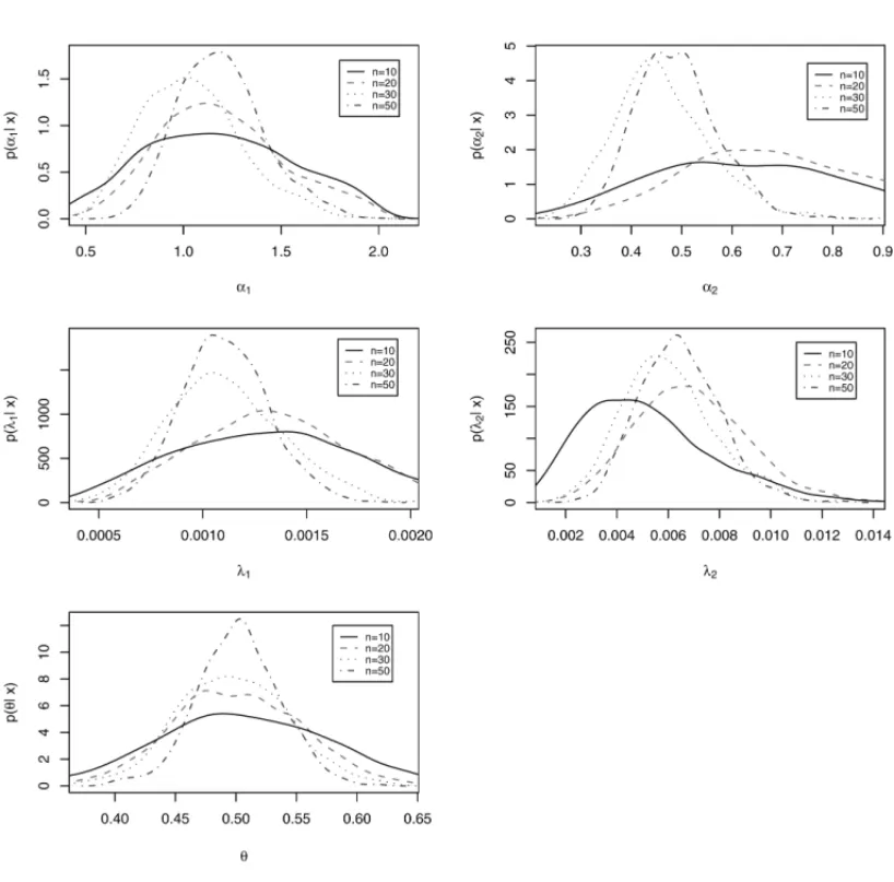
Figure 2– Marginal posterior densities for each parameter with different sample sizes,n =10, 20, 50 and 100.

From the results of Table 1, we observe that we get accurate Bayesian inferences for the eters of the model, especially considering large samples sizes. The only exception is the param-eterθ, where the 95% credible intervals are very large considering the four simulated samples (n=10,n=20,n=30 orn=50).

Figure 2 illustrates the performance of marginal posterior densities for each parameterα1,α2,

λ1, λ2 andθ when the sample size increase, that is, for n =10, 20, 50 and 100. From the plots of Figure 2, we observe that as the sample size increases, we have more accurate Bayesian inferences (see also Table 1).

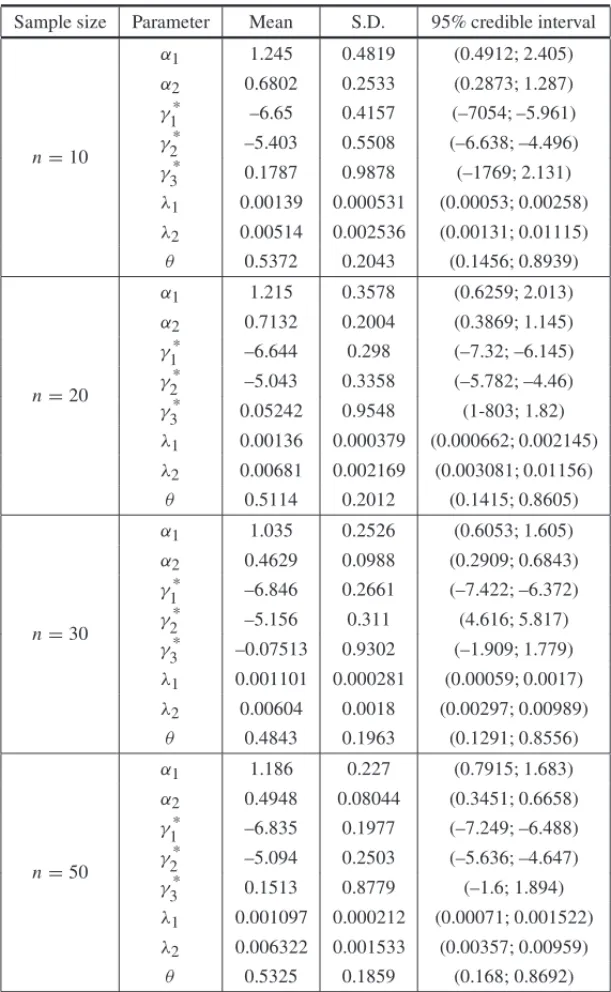
To improve the Bayesian inferences forθ, we could assume a transformation,γ∗

3 =log(

θ

1−θ),

consideringθpositive an assumption usually observed for the data (0< θ <1), the same prior distributions forγ₁∗,γ₂∗,α1andα2assumed for the results of Table 1 and a normal priorN(0,1) distribution forγ∗

From the results of Table 2, we observe similar posterior summaries for the parametersα1,α2,

γ∗

1,γ

∗

2,λ1andλ2as obtained in Table 1, but better accuracy for the Bayesian estimator forθ

as observed in the 95% credible intervals. We also observe that the accuracy of the Bayesian intervals for θ have some improvement as the data sample sizes increases, an indication of identifiability using the reparametrized form ofθ.

Table 2– Posterior summaries (simulated data set, logit transformation forθ).

Sample size Parameter Mean S.D. 95% credible interval

n=10

α1 1.245 0.4819 (0.4912; 2.405)

α2 0.6802 0.2533 (0.2873; 1.287)

γ₁* –6.65 0.4157 (–7054; –5.961)

γ₂* –5.403 0.5508 (–6.638; –4.496)

γ₃* 0.1787 0.9878 (–1769; 2.131)

λ1 0.00139 0.000531 (0.00053; 0.00258)

λ2 0.00514 0.002536 (0.00131; 0.01115)

θ 0.5372 0.2043 (0.1456; 0.8939)

n=20

α1 1.215 0.3578 (0.6259; 2.013)

α2 0.7132 0.2004 (0.3869; 1.145)

γ₁* –6.644 0.298 (–7.32; –6.145)

γ₂* –5.043 0.3358 (–5.782; –4.46)

γ₃* 0.05242 0.9548 (1-803; 1.82)

λ1 0.00136 0.000379 (0.000662; 0.002145)

λ2 0.00681 0.002169 (0.003081; 0.01156)

θ 0.5114 0.2012 (0.1415; 0.8605)

n=30

α1 1.035 0.2526 (0.6053; 1.605)

α2 0.4629 0.0988 (0.2909; 0.6843)

γ₁* –6.846 0.2661 (–7.422; –6.372)

γ₂* –5.156 0.311 (4.616; 5.817)

γ₃* –0.07513 0.9302 (–1.909; 1.779)

λ1 0.001101 0.000281 (0.00059; 0.0017)

λ2 0.00604 0.0018 (0.00297; 0.00989)

θ 0.4843 0.1963 (0.1291; 0.8556)

n=50

α1 1.186 0.227 (0.7915; 1.683)

α2 0.4948 0.08044 (0.3451; 0.6658)

γ₁* –6.835 0.1977 (–7.249; –6.488)

γ₂* –5.094 0.2503 (–5.636; –4.647)

γ₃* 0.1513 0.8779 (–1.6; 1.894)

λ1 0.001097 0.000212 (0.00071; 0.001522)

λ2 0.006322 0.001533 (0.00357; 0.00959)

The Bayesian estimation also performs well in applications with a large number of censored data. Table 3 shows the results of simulation studies for different sample sizes asn =10 (d1= 10,d2=5);n =20 (d1=12,d2=20);n =50 (d1 =30,d2 =20) andn =100 (d1 =30, d2=90).

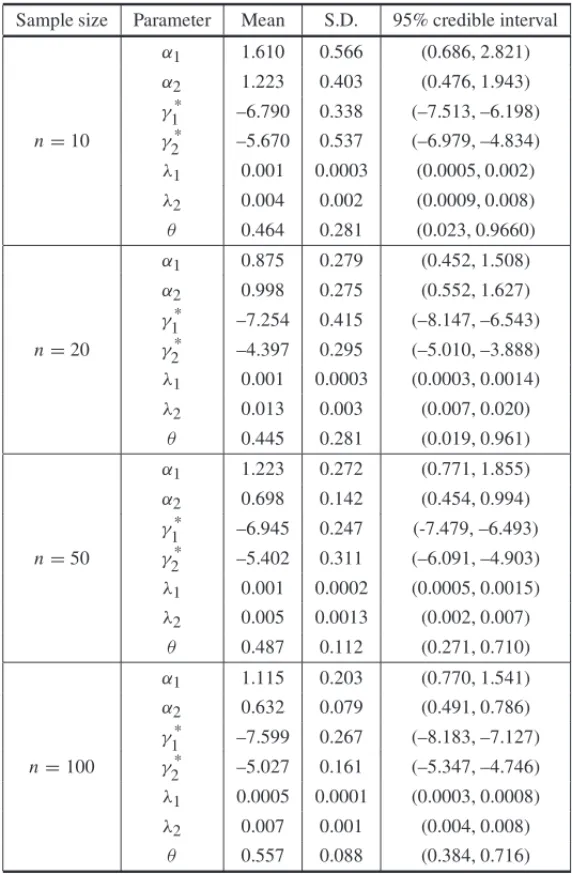
Table 3– Posterior summaries of simulated data set with high level of censoring.

Sample size Parameter Mean S.D. 95% credible interval

α₁ 1.610 0.566 (0.686, 2.821)

α2 1.223 0.403 (0.476, 1.943)

γ₁* –6.790 0.338 (–7.513, –6.198) n=10 γ₂* –5.670 0.537 (–6.979, –4.834)

λ1 0.001 0.0003 (0.0005, 0.002)

λ₂ 0.004 0.002 (0.0009, 0.008)

θ 0.464 0.281 (0.023, 0.9660)

α1 0.875 0.279 (0.452, 1.508)

α₂ 0.998 0.275 (0.552, 1.627)

γ₁* –7.254 0.415 (–8.147, –6.543) n=20 γ₂* –4.397 0.295 (–5.010, –3.888)

λ1 0.001 0.0003 (0.0003, 0.0014)

λ2 0.013 0.003 (0.007, 0.020)

θ 0.445 0.281 (0.019, 0.961)

α1 1.223 0.272 (0.771, 1.855)

α2 0.698 0.142 (0.454, 0.994)

γ₁* –6.945 0.247 (-7.479, –6.493) n=50 γ₂* –5.402 0.311 (–6.091, –4.903)

λ1 0.001 0.0002 (0.0005, 0.0015)

λ2 0.005 0.0013 (0.002, 0.007)

θ 0.487 0.112 (0.271, 0.710)

α1 1.115 0.203 (0.770, 1.541)

α2 0.632 0.079 (0.491, 0.786)

γ₁* –7.599 0.267 (–8.183, –7.127) n=100 γ₂* –5.027 0.161 (–5.347, –4.746)

λ₁ 0.0005 0.0001 (0.0003, 0.0008)

λ2 0.007 0.001 (0.004, 0.008)

θ 0.557 0.088 (0.384, 0.716)

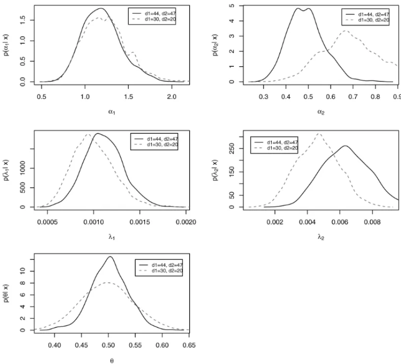
Figure 3 shows a comparison of the posterior distributions of each parameter in order to analyze the sensitivity of the estimation when the number of censored lifetime data is increased. We consider samples of sizen =50 with (d1=44,d2=47) and (d1 =30,d2=20). Despite the high degree of censoring, the performance of the estimates are quite similar for the parameters

α1,λ1andθ of the bivariate generalized exponential distribution. We note that the parameters

α2andλ2are more sensitive to censorship certainly due to the higher percentage of censorship occurred forT2variable, hence requiring a larger number of observations.

Figure 3– Marginal posterior densities for each parameter with different sample sizes,n=10, 20, 50 and 100 with high level of censoring.

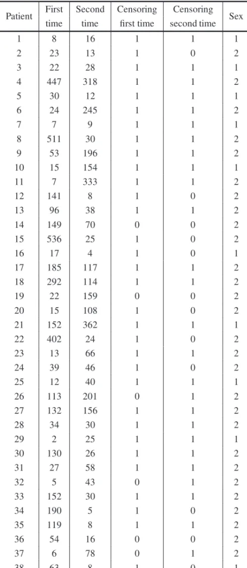
6.2 Recurrence times of infection for kidney patients

lifetime (in days) of the patient until an infection occurred and the catheter had to be removed, or the censoring time, where the catheter was removed by other reasons. The catheter is reinserted after some time and the second infection time is again observe or censored (data set in Table 4).

As a first analysis, let us assume the bivariate generalized exponential distribution with density (12) not considering the presence of the covariate sex. Let us devote this model as “model 1”.

For a Bayesian analysis of “model 1”, not considering the presence of the covariate sex, let us as-sume the same reparametrization forλ1,λ2andθconsidered in Section 6.1, that is,γ₁∗=log(λ1),

γ₂∗ = log(λ2)andγ₃∗ = log(₁₋θ_θ)(from a preliminary data analysis, the sample correlation between the lifetimes considering only the uncensored observations is given by 0.181; that is, we are assuming 0 < θ < 1), and the following prior distributions: γ₁∗ ∼ U(−10,0),

γ∗

2 ∼U(−10,0),α1∼U(0, 3),α2∼U(0,2)andγ

∗

3 ∼U(−1, 1).

Using the WinBugs software, we simulated 2000 Gibbs samples from the joint posterior dis-tribution of interest taking every 30th simulated sample after a “burn-in-sample” period of size 5000.

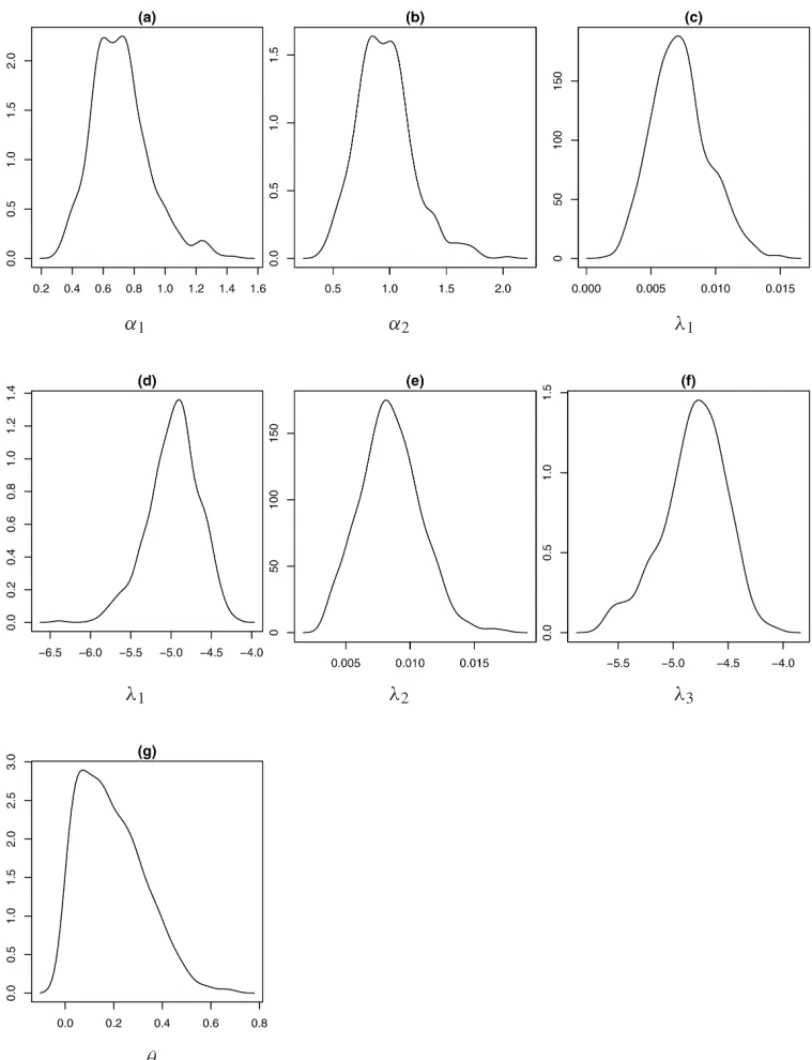
Convergence of the Gibbs sampling algorithm was monitored using standard existing methods as traceplots for the simulated samples. The posterior densities for each parameter are shown in Figure 4.

In Table 5, we have the posterior means, the posterior standard-deviations and 95% Bayesian intervals for the parameters of the model. We also have the MLE estimates and their asymptotical confidence intervals.

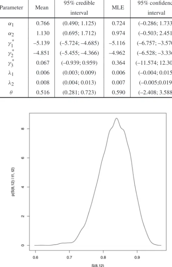
Often concern focusses on the survival functionS(t1,t2)given in (14). For instance, by using the priors proposed in this paper we haveP(T1 >8 days,T2 >12 days)=0.833 with a credible interval(0.737,0.914).

Figure 5 shows graphically the posterior distribution of the probabilityP(T1 >8 days,T2>12 days).

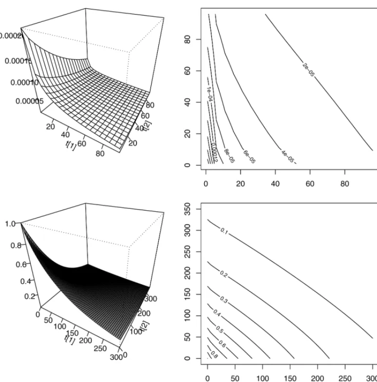
Finally, we derive the joint density and survival functions from the (12) and (14) respectively, for kidney infection in patients data and a plot of both functions is provided in Figure 6.

In the presence of the covariate sex, denoted byX, we assume the regression model introduced in Section 5, that is,

λ1i =γ1exp(β1xi) λ2i =γ2exp(β2xi)

(26)

wherei =1,2, . . . ,38;Xi =1 (male) andXi =0 (female) (see (24)). Let us denote this model as “model 2”.

Also assuming the reparametrizationγ∗

3 =log(

θ

1−θ), and the prior distributionsγj ∼U(0,1),

Table 4– Recurrence times of infections in 38 kidney patients.

Patient First Second Censoring Censoring Sex time time first time second time

1 8 16 1 1 1

2 23 13 1 0 2

3 22 28 1 1 1

4 447 318 1 1 2

5 30 12 1 1 1

6 24 245 1 1 2

7 7 9 1 1 1

8 511 30 1 1 2

9 53 196 1 1 2

10 15 154 1 1 1

11 7 333 1 1 2

12 141 8 1 0 2

13 96 38 1 1 2

14 149 70 0 0 2

15 536 25 1 0 2

16 17 4 1 0 1

17 185 117 1 1 2

18 292 114 1 1 2

19 22 159 0 0 2

20 15 108 1 0 2

21 152 362 1 1 1

22 402 24 1 0 2

23 13 66 1 1 2

24 39 46 1 0 2

25 12 40 1 1 1

26 113 201 0 1 2

27 132 156 1 1 2

28 34 30 1 1 2

29 2 25 1 1 1

30 130 26 1 1 2

31 27 58 1 1 2

32 5 43 0 1 2

33 152 30 1 1 2

34 190 5 1 0 2

35 119 8 1 1 2

36 54 16 0 0 2

37 6 78 0 1 2

α1 α2 λ1

λ1 λ2 λ3

θ

Figure 4– Marginal posterior densities for each parameter of “model 1”.

Table 5– Bayesian summaries (“model 1” not considering the covariate sex).

Parameter Mean 95% credible MLE 95% confidence

interval interval

α1 0.766 (0.490; 1.125) 0.724 (–0.286; 1.733)

α2 1.130 (0.695; 1.712) 0.974 (–0.503; 2.451)

γ₁* –5.139 (–5.724; –4.685) –5.116 (–6.757; –3.570)

γ₂* –4.851 (–5.455; –4.366) –4.962 (–6.528; –3.336)

γ₃* 0.067 (–0.939; 0.959) 0.364 (–11.574; 12.300)

λ₁ 0.006 (0.003; 0.009) 0.006 (–0.004; 0.015)

λ2 0.008 (0.004; 0.013) 0.007 (–0.005;0.019)

θ 0.516 (0.281; 0.723) 0.590 (–2.408; 3.588)

Figure 5– Posterior density of survivalS(8,12).

Figure 6– Plots and contours of bivariate functions for the “model 1”.

Table 6– Bayesian summaries (“model 2” in the presence of the covariate sex).

Parameter Posterior S.D. 95% credible

mean interval

α1 0.842 0.179 (0.588; 1.179)

α2 1.143 0.257 (0.771; 1.612)

λ1 0.006 0.001 (0.004; 0.009)

λ2 0.009 0.002 (0.005; 0.014)

β₁ 0.230 0.159 (–0.024; 0.514)

β₂ –0.118 0.147 (–0.345; 0.113)

7 CONCLUDING REMARKS

The use of bivariate generalized exponential distributions derived from copula functions could be a good alternative to analyze bivariate lifetime data, usually in the presence of censored obser-vations and covariates. Other copula functions also could be used to derive bivariate lifetime dis-tributions. Bayesian inference for this class of models using standard existing MCMC methods is a good alternative to get accurate inference results. It is important to point out that the depen-dence parameterθ can present some identifiability problems and this problem could be solved considering an informative prior fromθbased on expert opinion or considering a reparametriza-tion, as it was observed in this paper.

The use of existing Bayesian softwares like the WinBugs software gives a great simplification to get the posterior summaries of interest.

REFERENCES

[1] BLOCKH & BASUA. 1974. A Continuous bivariate exponential extension.Journal of the American

Statistical Association,69: 1031–1037.

[2] CASELLAG & GEORGEE. 1992. Explaining the Gibbs samples.The American Statistician, 46: 167–174.

[3] CHIBSE. 1995. Understanding the Metropolis-Hastings algorithm.The American Statistician, 49: 327–335.

[4] CLEMENRT, FISCHERGW & WINKLER RL. 2000. Assessing dependence: Some experimental results.Management Science,46: 1100–1115.

[5] DOWTONF. 1970. Bivariate exponential distributions in reliability theory.Journal of Royal Statistical

Society, B,32: 408–417.

[6] FREES EW & VALDEZ EA. 1998. Understanding Relationships Using Copulas.North American

Actuarial Journal,2: 1–25.

[7] FREUND J. 1961. A bivariate extension of the exponential distribution. Journal of the American

Statistical Association,56: 971–977.

[8] GELFANDAE & SMITHAFM. 1990. Sampling based approaches to calculating marginal densities.

Journal of the American Statistical Association,85: 398–409.

[9] GUMBELE. 1960. Bivariate exponential distributions.Journal of the American Statistical Associa-tion,55: 698–707.

[10] GUPTARD & KUNDUD. 1999. Generalized exponential distribution.Australian and New Zealand

Journal of Statistics,41: 173–188.

[11] GUPTA RD & KUNDUD. 2007. Generalized exponential distribution: existing results and same recent developments,Journal of Statistical Planning and Inference, DOI: 10.1016/j.jspi. 2007.03.030.

[12] GUPTARD & KUNDUD. 2008. Generalized exponential distribution: Bayesian inference.

Compu-tational Statistics and Data Analysis,52(4): 1873–1883.

[13] HAWKESA. 1972. A bivariate exponential distribution with application to reliability.Journal of the

[14] LAWLESSJ. 1982. Statistical model and methods for lifetime data. John Wiley. New York.

[15] MARSHALLA & OLKINI. 1976. A generalized bivariate exponential distribution.Journal of Applied

Probability,4: 291–302.

[16] MCGILCHISTC & AISBETTC. 1991. Regression with frailty in survival analysis.Bimetrics,47: 461–466.

[17] MORGENSTERND. 1956. Einfache Beispiele Zweidimensionaler Verteilungen.Mitteilingsblatt fur

Matgematische Statistik,8: 234–253.

[18] NELSENRB. 1999. An introduction to copulas. Springer-Verlag, New York.

[19] RAQAB MZ. 2002. Inferences for generalized exponential distribution based on record statistics.

Journal of Statistics Planning and Inference,104: 339–350.

[20] RAQABMZ & AHSARULLAHM. 2001. Estimation of the location and scale parameters of general-ized exponential distribution based on order statistics.Journal of Statistics Computation and Simula-tion,69: 109–124.

[21] SARHANAM. 2007. Analysis of incomplete, censored data in competing risks models with general-ized exponential distribution.IEEE Transactions on Reliability,56: 132–138.

[22] SARKARS. 1987. A continuous bivariate exponential distribution.Journal of the American Statistical

Association,82: 667–675.

[23] SKLARA. 1959. Fonctions de repartition `an-dimensions et leurs marges.Inst. Stat. University Paris, 8: 229–231.

[24] TRIVEDIPK & ZIMMERDH. 2005a. Copula Modelling, New Publishes.

[25] TRIVEDIPK & ZIMMERDH. 2005b. Copula modeling: an introduction to practicioneis.

Founda-tions and trends in econometrics,1(1): 1–111.

[26] SPIEGELHALTERDJ, BESTN, CARLINB & VAN DERLINDEA. 2002. Bayesian measures of model complexity and fit (with discussion).Journal of the Royal Statistical Society, B,64: 583–639.

[27] SPIEGELHALTERDJ, THOMASA, BESTNG & LUNND. 2003. Winbugs version 1.4 user manual, MRC Biostatistics Unit, Institute of Public Helath and department of epidemiology and public health, Imperial College, School of Medicine (http://www.mrc bsu.com.ac.uk/bugs).

[28] ZHENGG. 2002. Fisher information matrix in type II censored data from exponentiated exponential family.Biometrical Journal,44: 353–357.

APPENDIX

DEVIANCE INFORMATION CRITERION (DIC)

The Deviance Information Criterion (DIC) is a criterion specifically useful for selection model under the Bayesian approach where samples of the posterior distributions for the parameters of the model are obtained using MCMC methods.

The deviance is defined by,

D(θ)= −2 log L(θ)+c (A1)

The DIC criterion defined by Spirgelhalter (2002) is given by,

D I C=D(θ)+2nD (A2)