doi: 10.1590/0101-7438.2015.035.01.0039
CREDIT SCORING MODELING WITH STATE-DEPENDENT SAMPLE SELECTION: A COMPARISON STUDY
WITH THE USUAL LOGISTIC MODELING
Paulo H. Ferreira
1, Francisco Louzada
2*and Carlos Diniz
3Received September 1, 2012 / Accepted December 12, 2013
ABSTRACT.Statistical methods have been widely employed to assess the capabilities of credit scoring classification models in order to reduce the risk of wrong decisions when granting credit facilities to clients. The predictive quality of a classification model can be evaluated based on measures such as sensitivity, specificity, predictive values, accuracy, correlation coefficients and information theoretical measures, such as relative entropy and mutual information. In this paper we analyze the performance of a naive logistic regression model, a logistic regression with state-dependent sample selection model and a bounded logistic regression model via a large simulation study. Also, as a case study, the methodology is illustrated on a data set extracted from a Brazilian retail bank portfolio. Our simulation results so far revealed that there is no statistically significant difference in terms of predictive capacity among the naive logistic regression mod-els, the logistic regression with state-dependent sample selection models and the bounded logistic regres-sion models. However, there is difference between the distributions of the estimated default probabilities from these three statistical modeling techniques, with the naive logistic regression models and the bounded logistic regression models always underestimating such probabilities, particularly in the presence of bal-anced samples. Which are common in practice.
Keywords: classification models, naive logistic regression, logistic regression with state-dependent sample selection, bounded logistic regression, performance measures, credit scoring.
1 INTRODUCTION
The proper classification of applicants is of vital importance for determining the granting of credit facilities. Historically, statistical classification models have been used by financial institutions as a major tool to help on granting credit to clients.
*Corresponding author.
The consolidation of the use of classification models occurred in the 90s, when changes in the world scene, such as deregulation of interest rates and exchange rates, increase in liquidity and in bank competition, made financial institutions more and more worried about credit risk, i.e., the risk they were running when accepting someone as their client. The granting of credit started to be more important in the profitability of companies in the financial sector, becoming one of the main sources of revenue for banks and financial institutions in general. Due to this fact, this sector of the economy realized that it was highly recommended to increase the amount of allo-cated resources without losing the agility and quality of credits, at which point the contribution of statistical modeling is essential. For more details about the developments in the credit risk measurement literature over the 80s and 90s, see Altman & Saunders (1998).
Classification models for credit scoring are based on databases of relevant client information, with the financial performance of clients evaluated from the time when the client-company rela-tionship began as a dichotomic classification. The goal of credit scoring models is to classify loan clients to either good credit or bad credit (Lee et al., 2002; Scarpel & Milioni, 2002), predicting the bad payers (Lim & Sohn, 2007).
In this context, discriminant analysis, regression trees, logistic regression, logistic regression with state-dependent sample selection, bounded logistic regression and neural networks are among the most widely used classification models. In fact, logistic regression is still very used in building and developing credit scoring models (Desai et al., 1996; Hand & Henley, 1997; Sarlija et al., 2004). Generally, the best technique for all data sets does not exist but we can compare a set of methods using some statistical criteria. Therefore, the main thrust of this paper is to in-vestigate and compare the performance of the naive logistic regression (Hosmer & Lemeshow, 1989), the logistic regression with state-dependent sample selection and the bounded logistic regression (Cramer, 2004) using performance measures, in terms of a simulation study. The idea is to analyze the impact of disproportional samples on credit scoring models. Logistic regression with state-dependent sample selection is a statistical modeling technique used in cases where the sample considered to develop a model, i.e. the selected sample, contains only a portion, usually small, of the individuals who make up one of two study groups, in general the most frequent group. In credit scoring, for instance, the group of good payers is expected to be the predominant group. In short, this recent technique takes into account the principle of sample selection and makes a correction in the estimated default probability from a naive logistic regression model. On the other hand, the bounded logistic regression technique is commonly used in rare events studies and modifies the naive logistic regression model by adding a parameter that quantifies an upper limit for the probability of the event of interest.
variable using discriminant analysis. Thus Fisher’s approach can be seen as the starting point for developments and modifications of the methodologies used for granting of credit until today, where statistical techniques, such as discriminant analysis, regression analysis, probit analy-sis, neural networks and logistic regression, have been used and examined (Boyes et al., 1989; Greene, 1998; Banasik et al., 2001; Sarlija et al., 2004; Selau & Ribeiro, 2011). Particularly, considering state-dependent sample selection in order to make a correction in the estimated de-fault probability from a credit scoring model; and/or introducing a ceiling or maximum risk in order to provide a better model for the cases where the event of interest is rare (Cramer, 2004). Survival analysis is an expending area of research in credit scoring and can be applied to model the time to default, for instance (Andreeva et al., 2007; Bellotti & Crook, 2009).
The predictive quality of a credit scoring model can be evaluated based on measures such as sensitivity, specificity, correlation coefficients and information measures, such as relative entropy and mutual information (Baldi et al., 2000).
Generally, there is no overall best statistical technique used in building credit scoring models, so that the choice of a particular technique depends on the details of the problem, such as the data structure, the features used, the extent to which it is possible to segregate the classes by using those features, and the purpose of the classification (Hand & Henley, 1997). Most studies that made a comparison between different techniques tried to discover that the most recent/advanced credit scoring techniques, such as neural networks and fuzzy algorithms are better than the tradi-tional ones. Nevertheless, the more simple classification techniques, such as linear discriminant analysis and naive logistic regression, have a very good performance, which is in majority of the cases not statistically different from other techniques (Baesens et al., 2003; Hand, 2006).
This paper is organized as follows. Section 2 describes the three commonly used statistical techniques in building credit scoring models: the naive logistic regression, the logistic regression with state-dependent sample selection and the bounded logistic regression. Section 3 presents some useful measures that are used to analyze the predictive capacity of a classification model. Section 4 describes the details of a simulation study performed in order to compare the tech-niques of interest. In Section 5 the methodology is illustrated on a real data set from a Brazilian retail bank portfolio. Finally, Section 6 concludes the paper with some final comments.
2 CREDIT SCORING MODELS
In this Section, the three statistical techniques used for building credit scoring are described.
2.1 Naive Logistic Regression
status, age and income, as well as information about his credit product in use, such as number of parcels, purpose and credit value, are observed at the time the clients apply for the credit.
Let us consider a large sample of observations with predictorsxi and binary(0,1)outcomesYi.
Here, the eventYi =1 represents a bad credit, while the complementYi =0 represents a good
credit. The model specifies that the probability ofi being a bad credit as a function of thexi is
given by,
P
Yi =1|xi =pβ,xi=pi. (1)
In the case that (1) is a naive logistic regression model, pi is given by,
pi =
exp(x′
iβ)
1+exp(x′
iβ)
(2)
(see Hosmer & Lemeshow, 1989). Thus the objective of a naive logistic regression model in credit scoring is to determine the conditional probability of a specific client belonging to a class, for instance, the bad payers class, given the values of the independent variables of that credit applicant (Lee & Chen, 2005).
2.2 Logistic Regression with State-Dependent Sample Selection
Now let us consider the situation where the eventYi =1 represents a bad credit but it has a low
incidence, while the complementYi =0 represents a good credit but it is abundant.
Suppose we wish to estimateβfrom a selected sample, which is obtained by discarding a large part of the abundant zero observations for reasons of convenience. Assume also that the overall sample, hereafter full sample, is a random sample with sampling fraction α and that only a fractionγ of the zero observations, taken at random, is maintained. The probability that the elementihasYi =1 and it is included in the sample is given byαpi, but forYi =0 it is given by γ α(1−pi), wherepiis calculated from (2). Then, the probability that an element of the selected
sample hasYi =1 is given by, ˜
pi =
pi
pi+γ (1−pi)
. (3)
The sketch of the proof of (3) is given in Appendix A.
2.2.1 Estimation Procedure
The log-likelihood of the observed sample can be written in terms of p˜ias follows,
l(β, γ )=Yilogp˜i(β,xi, γ )+(Yi −1)logp˜i(β,xi, γ ). (4)
standard maximum likelihood methods. In the special case that (1) is a naive logistic regression model, p˜i is given by,
˜
pi =
exp(x′
iβ)
exp(x′
iβ)+γ
= 1/γ .exp(x
′
iβ)
1+1/γ .exp(x′
iβ)
= exp(x
′
iβ−lnγ )
1+exp(x′
iβ−lnγ )
. (5)
Thus the p˜i of the selected sample also obey a naive logistic regression model, and besides
the intercept the same parametersβ apply as in the full sample. If it is needed, the full sample intercept can be easily recovered by adding lnγ to the intercept of the selected sample.
2.3 Bounded Logistic Regression
The bounded logistic regression model is derived from the naive logistic regression model by introducing a parameterωwhich quantifies an upper limit, i.e. a ceiling for the probability of the event of interest. The model specifies that the probability ofibeing a bad credit as a function of thexiis given by,
p∗i =ω exp(x
′
iβ)
1+exp(x′
iβ)
, (6)
where 0< ω <1.
Model (6) was proposed by Cramer (2004) who fitted the naive logistic regression model, the complementary log-log model and the bounded logistic regression model to the database of a Dutch financial institution. These data showed a low incidence of the event of interest and the Hosmer-Lemeshow test indicated the bounded logistic regression as the best fitting model to describe the observed data. According to Cramer (2004), the parameterωhas the ability to absorb the impact of possible significant covariates excluded from the database.
2.3.1 Estimation Procedure
The log-likelihood of the observed sample can be written in terms ofpi∗as follows,
l(β,ω)=Yilogpi∗(β,xi,ω)+(Yi−1)logp˜i(β,xi, γ ). (7)
Therefore, the maximum likelihood estimates ofβ andωcan be obtained through numerical maximization of (7).
3 MODEL VALIDATION
After building a statistical model, it is important we evaluate it. Particularly, we can say that a good model is one which produces scores that can distinguish good from bad credits, since the objective is to previously identify such groups and treat them differently considering distinct relationship policies (Thomas et al., 2002).
as basic information in the database. There are therefore four possible results for each client: a) The result given by the classification model is a true-positive (TP). In other words, the model indicates that the client is a bad payer, which, in fact, he actually is; b) The result given by the classification model is a false-positive (FP). In other words, the model accuses the client of being a bad payer, which, in fact, he actually is not; c) The result given by the classification model is a false-negative (FN). In other words, the model classifies him as a good payer, which, in fact, he actually is not; d) The result given by the classification model is a true-negative (TN). In other words, the model classifies the client as a good payer, which, in fact, he actually is.
These four possible situations above are summarized in Table 1. Two of these results,TPandTN, can be seen as indicating that the proposed model “got it right” and are important measures of financial behavior. Of the other results that can be considered to indicate that the proposed model “got it wrong”, the one that gives aFNclassification is often the most important and deserves the most attention. If the classification given by the proposed model is negative, and the client is, in fact, a bad payer, granting to this client the credit requested can end up with the client defaulting, which, added to other cases of defaults by bad payers, can result in very high overall default rates for the company, and a real threat to its financial sustainability. AFPresult can also be negative for the company, since it may lose out by not approving credit for a client that would not, in fact, cause any default.
Table 1– Definitions used to validate classification models that produce dichotomized responses.
Result Real
from classification model positive(D+) negative(D−)
positive(M+) true-positive (TP) false-positive (FP) negative(M−) false-negative (FN) true-negative (TN)
The predictive capacity of a classification model is related to its performance measures, which can be calculated from Table 1. Among them we can cite sensitivity, specificity, positive and negative predictive values, accuracy, Matthews correlation coefficient, approximate correlation, relative entropy and mutual information.
Sensitivity (SEN) is defined as the probability that the classification model will produce a positive result, given that the client is a defaulter. In other words, sensitivity corresponds to the proportion of bad payers that are correctly classified by the classification model (Mazucheli et al., 2006), and is given by,
S E N =P(M+|D+)= T P
T P+F N. (8)
Specificity (SPE) is defined as the probability that a classification model will produce a negative result for a client who is not a defaulter. In other words, specificity represents the proportion of good payers that are correctly classified by the classification model (Mazucheli et al., 2006), and is calculated as follows,
S P E =P(M−|D−)= T N
Thus, a model with high sensitivity rarely fails to detect clients with the characteristic of interest (default) and a model with high specificity rarely classifies a client without this feature as a bad payer. According to Fleiss (1981) and Thibodeau (1981), it was J. Yerushalmy who, in 1947, first defined these measures and suggested they be used to evaluate classification models.
The Accuracy (ACC) is defined as the proportion of successes of a model, i.e. the proportion of true-positives and true-negatives in relation to all possible outcomes (Mazucheli et al., 2006). Accuracy is then given by,
ACC = T P+T N
T P+F P+T N+F N. (10)
The positive predictive value (PPV) of a model is defined as the proportion of bad payers identi-fied as such by the model, while the negative predictive value (NPV) of a model is defined as the proportion of good payers identified as such by the model (Mazucheli et al., 2006).
The positive and negative predictive values can be estimated directly from the sample, using the equations,
P PV = P(D+|M+)= T P
T P+F P (11)
and
N PV =P(D−|M−)= T N
F N+T N, (12)
respectively (Dunn & Everitt, 1995).
The more sensitive the model, the greater its negative predictive value. That is, the greater is the assurance that a client with a negative result is not a bad payer. Likewise, the more specific the model, the greater its positive predictive value. That is, the greater the guarantee of an individual with a positive result being a bad payer.
The correlation coefficient proposed by Matthews (1975) uses all four values (TP,FP,TN,TN) of a confusion matrix in its calculation. In general, it is regarded as a balanced measure which can be used even if the studied classes are of very different sizes. The Matthews correlation coef-ficient (MCC) returns a value between−1 and+1. A value of+1 represents a perfect prediction, i.e. total agreement, 0 a completely random prediction and−1 an inverse prediction, i.e. total disagreement. TheMCCis given by,
MCC =√ T P×T N−F P×F N
(T P+F P)×(T P+F N)×(T N +F P)×(T N+F N) (13)
(see Baldi et al., 2000).
Burset & Guig´o (1996) defined an approximate correlation measure to compensate for a declared problem with theMCC. That is, it is not defined if any of the four sumsTP+FN,TP+FP, TN+FP, orTN+FNis zero, e.g. when there are no positive predictions. They use the average conditional probability (ACP) which is defined as,
AC P = 1
4
T P
T P+F N +
T P
T P+F P +
T N
T N+F P +
T N
T N+F N
, (14)
if all the sums are non-zero; otherwise, it is the average over only those conditional probabilities that are defined. Approximate correlation (AC) is a simple transformation of theACPgiven by,
AC=2×(AC P −0.5). (15)
It returns a value between −1 and+1 and has the same interpretation as the MCC. Burset & Guig´o (1996) observe that theACis close to the real correlation value. However, some authors, like Baldi et al. (2000), do not encourage its use, since there is no simple geometrical interpreta-tion forAC.
Suppose thatD′=(d1, . . . ,dN)is a vector of true conditions of clients andM′=(m1, . . . ,mN)
a vector of predictions from a classification model, both binary (0,1). The dis and mis are
then equal to 0 or 1, for instance, 0 indicates a good payer and 1 a bad payer. The mutual information betweenDandMis measured by,
I(D,M) = −H
T P N , T N N , F P N , F N N −T P
N log(d¯m¯)−
F N
N log(d¯(1− ¯m))
− F P
N log((1− ¯d)m¯)−
T N
N log((1− ¯d)(1− ¯m))
(16)
(see Wang, 1994), whereNis the sample size,d¯=(T P+F N)/N,m¯ =(T P+F P)/N and
H T P N , T N N , F P N , F N N
= − T P
N log
T P
N
−T N
N log
T N
N
−F P
N log
F P
N
− F N
N log
F N
N
is the usual entropy, whose roots are in information theory (Kullback & Leibler, 1951; Kullback, 1959; Baldi & Brunak, 1998).
The mutual information always satisfies 0 ≤ I(D,M) ≤ H(D), whereH(D) = − ¯mlogm¯ − (1− ¯m)log(1− ¯m). Thus in the assessment of performance of a classification model, it is habitual to use the normalized mutual information coefficient (Rost & Sander, 1993; Rost et al., 1994), which is given by,
I C(D,M)= I(D,M)
H(D) . (17)
4 SIMULATION STUDY
In this Section, we present results of the performed simulation study. The simulation study was conducted to compare the performance of the naive logistic regression, the logistic regression with state-dependent sample selection and the bounded logistic regression. Here, we consid-ered some circumstances that may arise in the development of credit scoring models, and which involve the number of clients in the training sample and its degree of unbalance.
First, we generated a population of clients of a hypothetical credit institution, with the fol-lowing composition: 10,000,000 good payers and 100,000 bad payers. The data for good pay-ers were generated from a six-dimensional multivariate normal distribution, with mean vector µ′
B = (0, . . . ,0)and covariance matrix 4× I6, where I6 is the identity matrix of order 6;
while the data for bad payers were generated from a six-dimensional multivariate normal dis-tribution, with meanµ′M =
1/√6, . . . ,1/√6
and covariance matrix I6(Breiman, 1998). We categorized the six observed continuous covariates using the quartiles. Afterwards, we took out a stratified random sample (full sample) of 1,000,000 good payers (10% of the population size of this group) and 10,000 bad payers (10% of the population size of this class) of the generated population. Then the selected samples were obtained by keeping all bad payers of the full sam-ple, plus 10,000*Kgood payers taken out randomly from the full sample. Here, we studied only the cases whereK =1,3,9 and 19, which correspond to 10,000, 30,000, 90,000 and 190,000 good payers in the selected samples, respectively. For each K, we performed 100 simulations, i.e. 100 samples were obtained for eachK. In each one of them, the good payers were selected from their group in the full sample via simple random sampling without replacement.
For each obtained sample and for each K we applied the following procedures: a naive logis-tic regression model (Hosmer & Lemeshow, 1989), a logislogis-tic regression with state-dependent sample selection model and a bounded logistic regression model (Cramer, 2004) were fitted to the data and their predictive capacity was investigated in the training sample by the calculation of their performance measures.
After simulating for eachK, we obtained vectors of length 100, i.e. vectors with 100 records for each of the studied performance measures. Then we could obtain an average estimate for each measure by computing the mean value of each vector.
empirical curves for the distributions of estimated probabilities, original, adjusted or predicted from the bounded logistic regression models, by computing the mean value of each row. The simulations were performed using SAS version 9.0. Interested readers can email the authors for the codes.
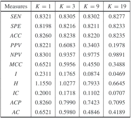
Tables 2, 3 and 4 show the empirical averages for the performance measures: naive logistic regression results are presented in Table 2, logistic regression with state-dependent sample se-lection results are presented in Table 3 and bounded logistic regression results are presented in Table 4. The empirical results presented in Table 2 reveal that the naive logistic regression tech-nique produces good results, with high values of positive and negative predictive values among others, only when the sample used for the development of the model is balanced, i.e. when K =1. As the degree of imbalance increases (K =3,K =9 andK =19) positive predictive value decreases considerably, assuming values less than 0.5 whenK =9 andK =19, whereas negative predictive value increases, reaching values near 1 forK =9 andK =19. Note that the values ofMCC,ICandACare also decreasing asKincreases.
Table 2– Empirical averages for the performance mea-sures, when we use the naive logistic regression technique.
Measures K =1 K =3 K =9 K=19
SEN 0.8321 0.8305 0.8302 0.8277
SPE 0.8198 0.8216 0.8211 0.8233
ACC 0.8260 0.8238 0.8220 0.8235
PPV 0.8221 0.6083 0.3403 0.1978
NPV 0.8301 0.9357 0.9775 0.9891
MCC 0.6521 0.5956 0.4550 0.3488
I 0.2311 0.1765 0.0874 0.0469
H 1.1550 1.0277 0.7933 0.6645
IC 0.2001 0.1718 0.1102 0.0707
ACP 0.8260 0.7990 0.7423 0.7095
AC 0.6521 0.5980 0.4846 0.4189
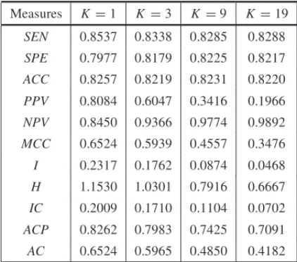
Discussions about the results of the logistic regression with state-dependent sample selection technique and bounded logistic regression technique (Tables 3 and 4 summarize these results, respectively) are analogous to those made previously, when we use the naive logistic regression technique.
Table 3– Empirical averages for the performance measures, when we use the logistic regression with state-dependent sample selection technique.
Measures K=1 K=3 K =9 K =19
SEN 0.8537 0.8338 0.8285 0.8288
SPE 0.7977 0.8179 0.8225 0.8217
ACC 0.8257 0.8219 0.8231 0.8220
PPV 0.8084 0.6047 0.3416 0.1966
NPV 0.8450 0.9366 0.9774 0.9892
MCC 0.6524 0.5939 0.4557 0.3476
I 0.2317 0.1762 0.0874 0.0468
H 1.1530 1.0301 0.7916 0.6667
IC 0.2009 0.1710 0.1104 0.0702
ACP 0.8262 0.7983 0.7425 0.7091
AC 0.6524 0.5965 0.4850 0.4182
Table 4– Empirical averages for the performance measures, when we use the bounded logistic regression technique.
Measures K=1 K=3 K =9 K =19
SEN 0.8322 0.8301 0.8271 0.8136
SPE 0.8195 0.8217 0.8236 0.8356
ACC 0.8258 0.8238 0.8239 0.8345
PPV 0.8218 0.6083 0.3425 0.2067
NPV 0.8301 0.9355 0.9772 0.9884
MCC 0.6518 0.5954 0.4561 0.3559
I 0.2309 0.1764 0.0874 0.0474
H 1.1552 1.0277 0.7905 0.6470
IC 0.1999 0.1717 0.1106 0.0733
ACP 0.8259 0.7989 0.7426 0.7111
AC 0.6518 0.5978 0.4852 0.4222
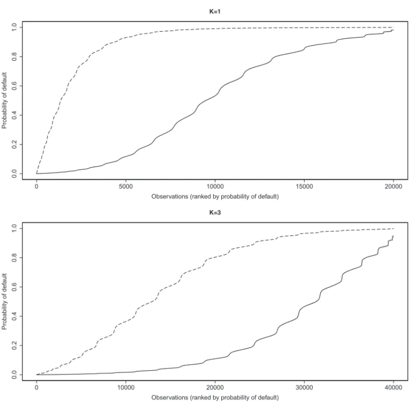
default. Note also that the distance among the curves decreases as the degree of sample im-balance increases. The curves are closer when the degree of imim-balance is close to the real one present in the full sample, that is, approximately 99% of good payers and 1% of bad payers. For instance, the distance between the curves is largest forK =1 (Fig. 1 upper panel), i.e. for bal-anced samples, while the curves are very close to each other forK =19 (Fig. 2 bottom panel), i.e. for 190,000 good payers and 10,000 bad payers in the selected samples.
0 5000 10000 15000 20000 0 .0 0 .2 0 .4 0 .6 0 .8 1 .0 K=1
Observations (ranked by probability of default)
Pro b a b ili ty o f d e fa u lt
0 10000 20000 30000 40000
0 .0 0 .2 0 .4 0 .6 0 .8 1 .0 K=3
Observations (ranked by probability of default)
Pro b a b ili ty o f d e fa u lt
Figure 1– Estimated cumulative probabilities, where —– represents the empirical curve for the original probability;− − −−represents the empirical curve for the adjusted probability; and· · · ·the empirical curve for the predicted probability from bounded logistic regression model. Upper panel:K=1 and lower panel:K =3.
5 BRAZILIAN RETAIL BANK CREDIT SCORING DATA
0 10000 20000 30000 40000 50000 0 .0 0 .2 0 .4 0 .6 0 .8 1 .0 K=9
Observations (ranked by probability of default)
Pro b a b ili ty o f d e fa u lt
0 10000 20000 30000 40000 50000
0 .0 0 .2 0 .4 0 .6 0 .8 1 .0 K=19
Observations (ranked by probability of default)
Pro b a b ili ty o f d e fa u lt
Figure 2– Estimated cumulative probabilities, where —– represents the empirical curve for the original probability;− − −−represents the empirical curve for the adjusted probability; and· · · · the empirical curve for the predicted probability from bounded logistic regression model. Upper panel:K =9 and lower panel:K=19.
by the good results in the simulation study) selected sample was obtained by maintaining all bad payers of the full sample, plus 122 good payers selected randomly from the full sample. Thus, a naive logistic regression model (Hosmer & Lemeshow, 1989), a logistic regression with state-dependent sample selection model and a bounded logistic regression model (Cramer, 2004) were applied to the balanced selected sample and then the test sample was used to analyze the appropriateness of the adjusted models.
and 0.46 for the naive logistic regression model, the logistic regression with state-dependent sample selection model and the bounded logistic regression model, respectively. In the Figure 3 right panel we observe the distributions of estimated default probabilities in the test sample from the three studied techniques. Note that the naive logistic regression model, which provides us the original probability of a client being a bad payer, and the bounded logistic regression model underestimate the probability of default. The measures of the predictive capacity of the adjusted models are showed in Table 5 for the balanced selected sample and test sample. Note that the measures of the three models are very close and are indicative of good predictive capacity, which is confirmed by the ROC curves (Fig. 3 left panel).
0.0 0.2 0.4 0.6 0.8 1.0
0 .0 0 .2 0 .4 0 .6 0 .8 1 .0 ROC Curves
1 − Specificity
Se n si ti vi ty
0 500 1000 1500
0 .0 0 .2 0 .4 0 .6 0 .8 1 .0
Cumulative Probabilities Curves
Observations (ranked by probability of default)
Pro b a b ili ty o f d e fa u lt
Figure 3– The ROC curves constructed from the training sample of a bank’s actual portfolio (panels on the left) and the corresponding distributions of estimated probabilities in an unbalanced test sample with 70% good payers and 30% bad payers (panels on the right). To the panels on the left, —– represents the naive logistic regression model;− − −−represents the logistic regression with state-dependent sample selection model; and· · · · the bounded logistic regression model. To the panels on the right, —– represents the original probability;− − −−represents the adjusted one; and· · · · the estimated probability from the bounded logistic regression model.
6 FINAL COMMENTS
Credit scoring techniques have become one of the most important tools currently used by fi-nancial institutions such as banks, in the measurement and evaluation of the loans credit risk. Furthermore, credit scoring is regarded as one of the basic applications of misclassification problems that have attracted most attention during the past decades.
Based on the simulation results, we discover that there is no difference between the cumula-tive distributions of the default estimated probabilities by the use of the naive logistic regression and bounded logistic regression techniques. However, there is difference between the default estimated probabilities from these two models and the predicted probabilities from the logis-tic regression with state-dependent sample selection model. Parlogis-ticularly, the naive logislogis-tic re-gression models and the bounded logistic rere-gression models underestimate such probabilities. Although there is no difference concerning to the performance of adjusted models from such techniques when we use measures like sensitivity, specificity and accuracy among others, in the evaluation of such models. The simulation study also showed that regardless of which of these three statistical modeling techniques is used, there is a need for working with balanced samples, which ensure models with good measures of positive and negative predictive values and high accuracy rate.
Table 5– The evaluation (performance measures) of the adjusted models in the balanced training sample and in the test sample (unbalanced with 70% good payers and 30% bad payers), where NLR is the naive logistic regres-sion model, LRSD is the logistic regresregres-sion with state-dependent sample selection model and BLR refers to the bounded logistic regression model.
Measures Balanced Selected Sample Test Sample NLR LRSD BLR NLR LRSD BLR
SEN 0.7602 0.7496 0.7675 0.7380 0.7232 0.7343
SPE 0.7708 0.7814 0.7635 0.7295 0.7409 0.7303
ACC 0.7655 0.7655 0.7655 0.7321 0.7355 0.7315
PPV 0.7683 0.7742 0.7644 0.5457 0.5513 0.5452
NPV 0.7627 0.7573 0.7666 0.8635 0.8588 0.8619
MCC 0.5310 0.5313 0.5310 0.4374 0.4363 0.4349
I 0.1485 0.1487 0.1485 0.0970 0.0959 0.0958
H 1.2377 1.2371 1.2378 1.1967 1.1932 1.1973
IC 0.1200 0.1202 0.1200 0.0810 0.0803 0.0800
ACP 0.7655 0.7656 0.7655 0.7192 0.7186 0.7179
AC 0.5310 0.5313 0.5310 0.4383 0.4371 0.4359
APPENDIX A
Sketch of the proof of (3). If the event Ii =1 means that elementi is included in the sample,
from the Bayesian Theorem (Baron, 1994), it is possible to see that,
˜
pi =P(Yi =1|Ii =1)=
P(Yi =1,Ii =1)
P(Yi =1,Ii =1)+P(Yi =0,Ii =1)
= αpi
αpi+γ α(1−pi) =
pi
pi+γ (1−pi)
,
completing the proof.
ACKNOWLEDGMENTS
The research is partially founded by CNPq, Brazil.
REFERENCES
[1] ABREU HJ. 2004.Aplicac¸˜ao de an´alise de sobrevivˆencia em um problema de credit scoring e comparac¸˜ao com a regress˜ao log´ıstica.Dissertac¸˜ao de Mestrado, DEs-UFSCar.
[2] ALTMANEI & SAUNDERSA. 1998. Credit risk measurement: Developments over the last 20 years.
Journal of Banking & Finance,21: 1721–1742.
[3] ANDREEVAG, ANSELL J & CROOKJ. 2007. Modelling profitability using survival combination scores.European Journal of Operational Research,183(3): 1537–1549.
[4] BAESENS B, GESTEL TV, VIAENE S, STEPANOVAM, SUYKENSJ & VANTHIENEN J. 2003. Benchmarking state-of-the-art classification algorithms for credit scoring. The Journal of the Operational Research Society,54(6): 627–635.
[5] BALDI P & BRUNAK S. 1998. Bioinformatics: the machine learning approach. MIT Press, Cambridge, MA.
[6] BALDIP, BRUNAKS, CHAUVINY, ANDERSENCAF & NIELSENH. 2000. Assessing the accuracy of prediction algorithms for classification: an overview.Bioinformatics Review,16(5): 412–424.
[7] BANASIK J, CROOKJ & THOMAS L. 2001. Scoring by usage.The Journal of the Operational Research Society,52(9): 997–1006.
[8] BARONJ. 1994.Thinking and Deciding(2 ed.). Oxford University Press, London.
[9] BELLOTTI T & CROOKJ. 2009. Credit Scoring with Macroeconomic Variables Using Survival Analysis.The Journal of the Operational Research Society,60(12): 1699–1707.
[10] BOYESWJ, HOFFMANDL & LOWSA. 1989. An econometric analysis of the bank credit scoring problem.Journal of Econometrics,40(1): 3–14.
[11] BREIMANL. 1998. Arcing classifiers.The Annals of Statistics,26(3): 801–849.
[12] BURSETM & GUIGO´R. 1996. Evaluation of gene structure prediction programs.Genomics,34(3): 353–367.
[14] DESAIVS, CROOKJN & OVERSTREETGA. 1996. A comparison of neural networks and linear scoring models in the credit union environment.European Journal of Operational Research,95(1): 24–37.
[15] DUNNG & EVERITTBS. 1995.Clinical biostatistics: an introduction to evidence based medicine. London: Edward Arnold.
[16] FISHERRA. 1936. The use multiple measurements in taxonomic problems.Annals of Eugenics,7(7): 179–188.
[17] FLEISSJL. 1981.Statistical methods for rates and proportions. New York: John Wiley.
[18] GREENEW. 1998. Sample selection in credit-scoring models.Japan and the World Economy,10(3): 299–316.
[19] HANDDJ. 2006. Classifier Technology and the Illusion of Progress.Statistical Science,21(1): 1–14.
[20] HANDDJ & HENLEYWE. 1997. Statistical classification methods in consumer credit scoring: A review.Journal of the Royal Statistical Society: Series A (Statistics in Society),160(3): 523–541.
[21] HOSMERWD & LEMESHOWS. 1989.Applied Logistic Regression.New York: John Wiley.
[22] KANGS & SHINK. 2000.Customer credit scoring model using analytic hierarchy process. Informs & Korms, Seoul, 2197–2204. Korea.
[23] KULLBACKS. 1959.Information Theory and Statistics.New York: John Wiley.
[24] KULLBACKS & LEIBLER RA. 1951. On information and sufficiency.Ann. Math. Stat., 22(1): 79–86.
[25] LEE T & CHENI. 2005. A two-stage hybrid credit scoring model using artificial neural networks and multivariate adaptive regression splines.Expert Systems with Applications,28(4): 743–752.
[26] LEET, CHIUC, LUC & CHENI. 2002. Credit scoring using the hybrid neural discriminant tech-nique.Expert Systems with Applications,23(3): 245–254.
[27] LIMMK & SOHNSY. 2007. Cluster-based dynamic scoring model.Expert Systems with Applica-tions,32(2): 427–431.
[28] MATTHEWSBW. 1975. Comparison of the predicted and observed secondary structure of T4 phage lysozyme.Biochim. Biophys. Acta,405: 442–451.
[29] MAZUCHELIJA, LOUZADA-NETOF & MARTINEZEZ. 2008. Algumas medidas do valor preditivo de um modelo de classificac¸˜ao.Rev. Bras. Biom.,26(2): 83–91.
[30] ROSTB & SANDERC. 1993. Prediction of protein secondary structure at better than 70% accuracy.
J. Mol. Biol.,232(2): 584–599.
[31] ROSTB, SANDERC & SCHNEIDERR. 1994. Redefining the goals of protein secondary structure prediction.J. Mol. Biol.,235(1): 13–26.
[32] SARLIJAN, BENSICM & BOHACEKZ. 2004.Multinomial model in consumer credit scoring.10th International Conference on Operational Research. Trogir: Croatia.
[33] SCARPELRA & MILIONIAZ. 2002. Utilizac¸˜ao conjunta de modelagem econom´etrica e otimizac¸˜ao em decis ˜oes de concess˜ao de cr´edito.Pesquisa Operacional,22(1): 61–72.
[34] SELAULPR & RIBEIROJLD. 2011. A systematic approach to construct credit risk forecast models.
[35] THIBODEAULA. 1981. Evaluating diagnostic tests.Biometrics,37(4): 801–804.
[36] THOMASLC. 2000.A survey of credit and Behavioural Scoring; Forecasting financial risk of lending to consumers. University of Edinburgh, Edinburgh, U.K.
[37] THOMASLC, EDELMANDB & CROOKJN. 2002.Credit Scoring and Its Applications. Philadelphia: SIAM.