www.soil-journal.net/2/659/2016/ doi:10.5194/soil-2-659-2016
© Author(s) 2016. CC Attribution 3.0 License.
SOIL
Three-dimensional soil organic matter distribution,
accessibility and microbial respiration in
macroaggre-gates using osmium staining
and synchrotron X-ray computed tomography
Barry G. Rawlins1, Joanna Wragg1, Christina Reinhard2, Robert C. Atwood2, Alasdair Houston3, R. Murray Lark1, and Sebastian Rudolph1
1British Geological Survey, Keyworth, Nottingham, NG12 5GG, UK
2Diamond Light Source, Harwell Science & Innovation Campus, Chilton, OX11 0DE, UK
3SIMBIOS, Abertay University, 40 Bell Street, Dundee DD1 1HG, UK
Correspondence to:Barry G. Rawlins ([email protected])
Received: 15 April 2016 – Published in SOIL Discuss.: 25 April 2016
Revised: 21 October 2016 – Accepted: 15 November 2016 – Published: 15 December 2016
Abstract. The spatial distribution and accessibility of organic matter (OM) to soil microbes in aggregates – determined by the fine-scale, 3-D distribution of OM, pores and mineral phases – may be an important control on the magnitude of soil heterotrophic respiration (SHR). Attempts to model SHR on fine scales requires data on the transition probabilities between adjacent pore space and soil OM, a measure of microbial accessibility to the latter. We used a combination of osmium staining and synchrotron X-ray computed tomography (CT) to determine the 3-D (voxel) distribution of these three phases (scale 6.6 µm) throughout nine aggregates taken from a single soil core (range of organic carbon (OC) concentrations: 4.2–7.7 %). Prior to the synchrotron analyses we had measured the magnitude of SHR for each aggregate over 24 h under controlled conditions (moisture content and temperature). We test the hypothesis that larger magnitudes of SHR will be observed in aggregates with (i) shorter length scales of OM variation (more aerobic microsites) and (ii) larger transition probabilities between OM and pore voxels.
After scaling to their OC concentrations, there was a 6-fold variation in the magnitude of SHR for the nine ag-gregates. The distribution of pore diameters and tortuosity index values for pore branches was similar for each of the nine aggregates. The Pearson correlation between aggregate surface area (normalized by aggregate volume)
and normalized headspace C gas concentration was both positive and reasonably large (r=0.44), suggesting that
the former may be a factor that influences SHR. The overall transition probabilities between OM and pore voxels were between 0.07 and 0.17, smaller than those used in previous simulation studies. We computed the length scales over which OM, pore and mineral phases vary within each aggregate using 3-D indicator variograms. The median range of models fitted to variograms of OM varied between 38 and 175 µm and was generally larger
than the other two phases within each aggregate, but in general variogram models had ranges<250 µm. There
was no evidence to support the hypotheses concerning scales of variation in OM and magnitude of SHR; the linear correlation was 0.01. There was weak evidence to suggest a statistical relationship between voxel-based
OM–pore transition probabilities and the magnitudes of aggregate SHR (r=0.12). We discuss how our analyses
1 Introduction
In soil heterotrophic respiration (SHR) microbes utilize the carbon in soil organic matter (SOM) as an energy source,
releasing gaseous CO2, which accumulates in the soil at
sig-nificantly larger concentrations than in the atmosphere
(Hi-rano et al., 2003). Ultimately this excess CO2is released to
the global atmosphere. It is important we understand the pro-cesses that determine variations in the magnitude of SHR
be-cause it influences the flux of carbon dioxide (CO2) from
soils to the atmosphere, an important part of the global car-bon cycle with major implications for global climate change (Cox et al., 2000). The turnover of SOM is also an impor-tant control on the cycling of other macronutrients, notably nitrogen.
It has been suggested that it is essential to understand the influence of microscale intra-aggregate heterogeneity of soil properties to ensure that organic matter (OM) mineraliza-tion can be modelled effectively (Falconer et al., 2015). The majority of soil microbial communities reside in pore net-works within soil aggregates which are three-dimensional (3-D) agglomerations of mineral particles, varying in size, that form a hierarchy (Tisdall and Oades, 1982) with small
micro-aggregates (<250 µm) forming larger
macroaggre-gates (>250 µm). Soil aggregates consist of complex
mix-tures of SOM, mineral particles, pore space, microbes and moisture. The accessibility of SOM to microbial communi-ties (substrate availability) is determined by the distribution of pores (Chenu et al., 2001; Negassa et al., 2015), which also determines water potential and the flux of oxygen. Soil ma-tric potentials vary over short scales due to the varying size of pores, with microbes concentrated at the interfaces between air and water. Decomposition rates of SOM may therefore be influenced by moisture content (Moyano et al., 2012), pore size and location within an aggregate (Killham et al., 1993) and also by temperature and substrate quality (Davidson and Janssens, 2006) and microbial properties (Li et al., 2015).
The majority of SOM utilized by soil microbes, the former both as large individual particles and more finely dissemi-nated material associated with minerals, occurs both on the surfaces of, and within, soil aggregates (Leue et al., 2010). In controlled laboratory experiments, the magnitude of SHR has been shown to vary considerably between soil aggregates (Kravchenko et al., 2015). It has been suggested that the loca-tion of OM within soil aggregates may be a significant factor governing the magnitude of OM mineralization in soil (Dun-gait et al., 2012). Microsites for aerobic SHR occur where SOM and pores are adjacent to one another in soil aggre-gates, but to date their frequency and spatial distribution have not been established within macroaggregates. If a large pro-portion of intra-aggregate SOM is occluded by minerals so that microbes cannot utilize it, there will be fewer interfaces between SOM and pores and the magnitude of SHR for such aggregates may be smaller than those in which SOM is more accessible (a larger proportion of pore–SOM interfaces). In
a recent study, Juarez et al. (2013) asserted that soil struc-ture may be of limited importance in determining rates of SHR on the scale of the soil core. The authors created soils with differing structural properties (undisturbed versus dis-aggregated and sieved) and showed that after the structural perturbations had dissipated, there were no significant differ-ences in SHR rates for both native and added soil carbon. However, the observed increase in rates of SHR following disturbance also implies that soil structure does exert an in-fluence on rates of microbial SOM mineralization.
Another feature of soil aggregates that may influence the magnitude of SHR is the size and distribution of its SOM in-cluding particulate organic matter (Kravchenko et al., 2015). Consider two aggregates, with the same concentration of SOM, removed from a single soil core. In the first aggre-gate the SOM consists of small, finely disseminated material that occurs frequently over short length scales, whilst in the second there are fewer, larger particles of SOM with larger distances separating them. We hypothesize that in the former aggregate there will likely be a larger number of microsites leading to a greater magnitude of SHR compared to the latter. This hypothesis could be tested by determining the magni-tude of SHR in such aggregates if it were also possible to sub-sequently determine the length scales over which the SOM is distributed in these aggregates. Although the statistical meth-ods are well established for doing so, there are currently few laboratory methods for establishing the 3-D spatial variation of intra-aggregate OM distribution (see below).
To date, relatively few experimental approaches have been applied to determine (i) the accessibility of soil OM in macroaggregates and (ii) whether the accessibility of SOM in soil aggregates exerts a strong influence on microbial SHR on the macroaggregate scale. This is in part because
scien-tists have lacked methods for fine (<10 µm) scale 3-D
dis-crimination between minerals and SOM within aggregates. Approaches to date have generally been limited to mapping SOM in two dimensions (Lehmann et al., 2007) or in 3-D within smaller regions of aggregates (Yu et al., 2016). In a recent study, Hapca et al. (2015) used a combination of X-ray computed tomography (CT) and scanning electron mi-croscope images to map soil chemical composition, includ-ing soil carbon, at a resolution of 15.8 µm in a small block of soil (side length of 1 cm). An alternative approach was re-cently demonstrated by Peth et al. (2014), where differences in X-ray absorption above and below the osmium (Os) edge – using synchrotron beamline X-ray CT – were used to dis-criminate between OM and mineral phases in aggregates of around 2–3 mm diameter, at a resolution of 9.77 µm.
over which SOM, minerals and pores vary both within and between aggregates. In so doing we establish the magnitude of any structural differences between the nine aggregates. Prior to the synchrotron X-ray CT analyses we measured the magnitude of SHR of each aggregate in the laboratory
by measuring headspace CO2 concentrations after
incubat-ing the aggregates in separate vials, havincubat-ing controlled for both temperature and moisture content. We have determined the accessibility of SOM within each aggregate by comput-ing the transition probabilities between adjacent SOM and pore voxels and also the diameter and tortuosities of the pore networks. We used the SOM–pore transition probabilities as an index of SOM accessibility to determine whether it is strongly related to the magnitude of SHR for each aggre-gate, the latter scaled by total organic carbon (TOC) content. We also computed the length scales over which SOM varies in each aggregate and compared this to their magnitudes of SHR, again scaled by aggregate TOC content. We discuss the implications of our findings for empirical and modelling studies which aim to (respectively) quantify and simulate the magnitude of SHR on the macroaggregate scale.
2 Materials and methods
2.1 Aggregate samples, preparation and respiration measurements
An intact cylindrical core of soil (diameter and length 50 mm) was collected from a field that had been under pas-ture for more than 15 years (British National Grid reference metres; E 463 374, N 331 992) in Keyworth (near Notting-ham, UK). The upper edge of the soil cylinder was inserted (at a depth of 5 cm below the top of the mineral soil horizon) into a vertical soil face that had been exposed with a spade (the lower level of the cylinder was at a depth of 10 cm be-low the top of the mineral horizon). The parent material of the soil at this site is a mudstone and the soil is a Luvisol (World Reference Base, 2007) in texture class Clay (Hodg-son, 1974) based on a particle size analysis of material from a soil core collected from a location adjacent to the sampling site. After return to the laboratory (at room temperature) the intact core was removed from its container and placed on a plastic sheet. The core was broken apart by hand to sepa-rate large aggregates along natural fracture surfaces and also those formed by fine roots. This procedure yielded gates of different sizes. We selected a subset of nine aggre-gates which had shapes that were approximately either cubes or spheres with (respectively) side length or diameter of ap-proximately 5–6 mm. We visually inspected each aggregate and rejected any which appeared to be dominated by a large single particle (e.g. a stone fragment).
We weighed each aggregate in a preweighed and labelled weighing boat and then placed each on a saturated 1 bar pressure plate (Soil Moisture Equipment Corp, Santa Bar-bara, CA) for 20 min so that the moisture content of each
Filter Aggregate Silica beads Gas sample
headspace
Micro-vial Osmium
tetroxide
Freeze-dry
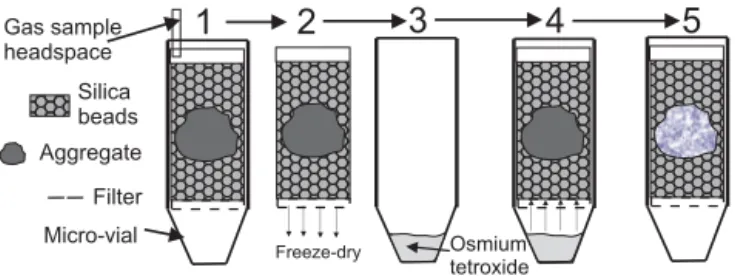
Figure 1.Schematic diagram showing a series of five steps in the treatment of the aggregates in their vials: (1) headspace gas removal, (2) freeze-drying, (3) and (4) staining with OsO4, and (5) scanning
in the synchrotron beamline.
aggregate would increase markedly. We then set the
pres-sure plate to 0.5 bar (−50 kPa) for 5 h so that each aggregate
had the same moisture content, i.e. slightly less than field capacity. After removal from the pressure plate the aggre-gates were placed inside a filter insert (Costar (R) Spin-X Centrifuge Tube, Sigma-Aldrich, UK) which had been par-tially filled with 500 µm quartz beads (Sigma Aldrich, UK). A further small quantity of quartz beads was added to en-sure each aggregate was surrounded and the insert (includ-ing quartz beads and aggregate) was reweighed. We added quartz beads to prevent the aggregates from fragmenting at either the freeze-drying stage or during transport to and from the synchrotron.
The filter inserts were then placed inside glass headspace vials (Thames Restek, Pennsylvania, USA), each of which had been filled with an equal quantity of quartz beads to re-duce the volume of air in the vial. A crimping tool was used to seal the headspace vials with an aluminium seal and the
vials were placed in an incubator at 37◦C for 24 h. After
re-moval of the vials from the incubator, the concentration of
CO2in the headspace of each vial was determined by
remov-ing a 0.5 cm3 subsample of gas using a syringe and
inject-ing it into a gas chromatograph (porapak column Q 80/100 mesh in Agilent GC 7820) which had been calibrated with
CO2standards of 100, 500, 1000 and 2000 mg L−1. We
sub-tracted the background concentration of CO2(400 mg L−1)
from each headspace analysis to give the excess CO2due to
respiration. The septa and seals were then removed from the headspace vials and the aggregate and filter holder placed into a Costar (R) Spin-X Centrifuge Tube (total volume 2 mL; see Fig. 1). The uncapped centrifuge tubes were placed in a freeze-drying unit for 48 h until any moisture in the vials had been removed completely. By removing all
mois-ture from the aggregates we wanted to ensure that the OsO4
2.2 Osmium staining of soil organic matter
The aggregates (each inside a filter insert and centrifuge vial) were placed inside a fume cupboard so that osmium
tetrox-ide (OsO4) could be used to stain the OM in each of the
soil aggregates (Peth et al., 2014). A set of strict health and safety procedures were adopted due to the hazardous nature
of OsO4, but we do not describe these in detail here. Half a
millilitre of OsO4was pipetted into the bottom of each
cen-trifuge vial, and the vials were sealed with caps. Each was left for 48 h inside the fume cupboard during which time the Os diffused through the base of the filter and through the glass beads and Os was adsorbed preferentially by the carbon bonds in the OM. A schematic diagram showing the main steps in this procedure is shown in Fig. 1.
The filter inserts were then removed and wiped clean and the top of each filter insert was sealed using caps and Araldite resin. Each filter insert was then fixed to bespoke stainless steel supports using Araldite resin so that the filters could be placed into a synchrotron beamline.
2.3 Synchrotron X-ray CT analysis
Each of the nine aggregates inside the filter inserts were scanned using synchrotron X-ray CT at the Diamond Light Source (Harwell, UK) using the I12 beamline. Each ag-gregate was scanned at three energy levels: 53, 73.2 and 74.4 keV; the latter were determined to be just below and above the K-absorption edge for Os, based on initial scan-ning of an osmium standard material. The 53 keV energy level provided an effective means of separating the solid and pore phases. The images for each horizontal slice through the aggregates were reconstructed, yielding a set of 32 bit .tif files in which each pixel has an adsorption value for each en-ergy level, and each pixel represents a 3-D voxel with a side length of 3.3 µm.
2.4 Total organic carbon content of aggregates
After the aggregates had been scanned in the beamline, they were carefully removed from their vials and their TOC con-tent was estimated using a Elementar Vario Max C/N
anal-yser at 1050◦C. Prior to measurement any inorganic carbon
was removed from the soil aggregates by adding HCl (5.7 M)
and was then dried at 100◦C for 1 h. The limit of
quantifica-tion for TOC for a typical 300 mg sample was 0.18 %.
2.5 Synchrotron X-ray CT data processing
All the synchrotron X-ray CT data were processed using the same protocol described here. The first procedure was to sub-tract the absorption values from the 73.2 keV energy level (below the Os absorption edge) from the images created from the 74.4 keV energy level (above the Os absorption edge; see Peth et al., 2014). This was undertaken using a script written in R (R Core Team, 2013), and we subsequently refer to the
● ● ● ● ● ● ● ● ● ● ● ● ● ● ● ● ● ● ● ● ● ● ● ● ● ● ● ● ● ● ● ● ● ● ● ● ● ● ● ● ● ● ● ● ● ● ● ● ● ● ● ● ● ● ● ● ● ● ● ● ● ● ● ● ● ● ● ● ● ● ● ● ● ● ● ● ● ● ● ● ● ● ● ● ● ● ● ● ● ● ● ● ● ● ● ● ● ● ● ● ● ● ● ● ● ● ● ● ● ● ● ● ● ● ● ● ● ● ● ● ● ● ● ● ● ● ● ● ● ● ● ● ● ● ● ● ● ● ● ● ● ● ● ● ● ● ● ● ● ● ● ● ● ● ● ● ● ● ● ● ● ● ● ● ● ● ● ● ● ● ● ● ● ● ● ● ● ● ● ● ● ● ● ● ● ● ● ● ● ● ● ● ● ● ● ● ● ● ● ● ● ● ● ● ● ● ● ● ● ● ● ● ● ● ● ● ● ● ● ● ● ● ● ● ● ● ● ● ● ●● ● ● ● ● ● ● ● ● ● ● ● ● ● ● ● ● ● ● ● ● ● ● ● ● ● ● ● ● ● ● ● ● ● ● ● ● ● ● ● ● ● ● ● ● ● ● ● ● ● ● ● ● ● ● ● ● ● ● ● ● ● ● ● ● ● ● ● ● ● ● ● ● ● ● ● ● ● ● ● ● ● ● ● ● ● ● ● ● ● ● ● ● ● ● ● ● ● ● ● ● ● ● ● ● ● ● ● ● ● ● ● ● ● ● ● ● ● ● ● ● ● ● ● ● ● ● ● ● ● ● ● ● ● ● ● ● ● ● ● ● ● ● ● ● ● ● ● ● ● ● ● ● ● ● ● ● ● ● ● ● ● ● ● ● ● ● ● ● ● ● ● ● ● ● ● ● ● ● ● ● ● ● ● ● ● ● ● ● ● ● ● ● ● ● ● ● ● ● ● ● ● ● ● ● ● ● ● ● ● ● ● ● ● ● ● ● ● ● ● ● ● ● ● ● ● ● ● ● ● ● ● ● ● ● ● ● ● ● ● ● ● ● ● ● ● ● ● ● ● ● ● ● ● ● ● ● ● ● ● ● ● ● ● ● ● ● ● ● ● ● ● ● ● ● ● ● ● ● ● ● ● ● ● ● ● ● ● ● ● ● ● ● ● ● ● ● ● ● ● ● ● ● ● ● ● ● ● ● ● ● ● ● ● ● ● ● ● ● ● ● ● ● ● ● ● ● ● ● ● ● ● ● ● ● ● ● ● ● ● ● ● ● ● ● ● ● ● ● ● ● ● ● ● ● ● ● ● ● ● ● ● ● ● ● ● ● ● ● ● ● ● ● ● ● ● ● ● ● ● ● ● ● ● ● ● ● ● ● ● ● ● ● ● ● ● ● ● ● ● ● ● ● ● ● ● ● ● ● ● ● ● ● ● ● ● ● ● ● ● ● ● ● ● ● ● ● ● ● ● ● ● ● ● ● ● ● ● ● ● ● ● ● ● ● ● ● ● ● ● ● ● ● ● ● ● ● ● ● ● ● ● ● ● ● ● ● ● ● ● ● ●● ● ● ● ● ● ● ● ● ● ● ● ● ● ● ● ● ● ● ● ● ● ● ● ● ● ● ● ● ● ● ● ● ● ● ● ● ● ● ● ● ● ● ● ● ● ● ● ● ● ● ● ● ● ● ● ● ● ● ● ● ● ● ● ● ● ● ● ● ● ● ● ● ● ● ● ● ● ● ● ● ● ● ● ● ● ● ●● ● ● ● ● ● ● ● ● ● ● ● ● ● ● ● ● ● ● ● ● ● ● ● ● ● ● ● ● ● ● ● ● ● ● ● ● ● ● ● ● ● ● ● ● ● ● ● ● ● ● ● ● ● ● ● ● ● ● ● ● ● ● ● ● ● ● ● ● ● ● ● ● ● ● ● ● ● ● ● ● ● ● ● ● ● ● ● ● ● ● ● ● ● ● ● ● ● ● ● ● ● ● ● ● ● ● ● ● ●● ● ● ● ● ● ● ● ● ● ● ● ● ● ● ● ● ● ● ● ● ● ● ● ● ● ● ● ● ● ● ● ● ● ● ● ● ● ● ● ● ● ● ● ● ● ● ● ● ● ● ● ● ● ● ● ● ● ● ● ● ● ● ● ● ● ● ● ● ● ● ● ● ● ● ● ● ● ● ● ● ● ● ● ● ● ● ● ● ● ● ● ● ● ● ● ● ● ● ● ● ● ● ● ● ● ● ● ● ● ● ● ● ● ● ● ● ● ● ● ● ● ● ● ● ● ● ● ● ● ● ● ● ● ● ● ● ● ● ● ● ● ● ● ● ● ● ● ● ● ● ● ● ● ● ● ● ● ● ● ● ● ● ● ● ● ● ● ● ● ● ● ● ● ● ● ● ● ● ● ● ● ● ● ● ● ● ● ● ● ● ● ● ● ● ● ● ● ● ● ● ● ● ● ● ● ● ● ● ● ● ● ● ● ● ● ● ● ● ● ● ● ● ● ● ● ● ● ● ● ● ● ● ● ● ● ● ● ● ● ● ● ● ● ● ● ● ● ● ● ● ● ● ● ● ● ● ● ● ● ● ● ● ● ● ● ● ● ● ● ● ● ● ● ● ● ● ● ● ● ● ● ● ● ● ● ● ● ● ● ● ● ● ● ● ● ● ● ● ● ● ● ● ● ● ● ● ● ● ● ● ● ● ● ● ● ● ● ● ● ● ● ● ● ● ● ● ● ● ● ● ● ● ● ● ● ● ● ● ● ● ● ● ● ● ● ● ● ● ● ● ● ● ● ● ● ● ● ● ● ● ● ● ● ● ● ● ● ● ● ● ● ● ● ● ● ● ● ● ● ● ● ● ● ● ● ● ● ● ● ● ● ● ● ● ● ● ● ● ● ● ● ● ● ● ● ● ● ● ● ● ● ● ● ● ● ● ● ● ● ● ● ● ● ● ● ● ● ● ● ● ● ● ● ● ● ● ● ● ● ● ● ● ● ● ● ● ● ● ● ● ● ● ● ● ● ● ● ● ● ● ● ● ● ● ● ● ● ● ● ● ● ● ● ● ● ● ● ● ● ● ● ● ● ● ● ● ● ● ● ● ● ● ● ● ● ● ● ● ● ● ● ● ● ● ● ● ● ● ● ● ● ● ● ● ● ● ● ● ● ● ● ● ● ● ● ● ● ● ● ● ● ● ● ● ● ● ● ● ● ● ● ● ● ● ● ● ● ● ● ● ● ● ● ● ● ● ● ● ● ● ● ● ● ● ● ● ● ●● ● ● ● ● ● ● ● ● ● ● ● ● ● ● ● ● ● ● ● ● ● ● ● ● ● ● ● ● ● ● ● ● ● ● ● ● ● ● ● ● ● ● ● ● ● ● ● ● ● ● ● ● ● ● ● ● ● ● ● ●● ● ● ● ● ● ● ● ● ● ● ● ● ● ● ● ● ● ● ● ● ● ● ● ● ● ● ● ● ● ● ● ● ● ● ● ● ● ● ● ● ● ● ● ● ● ● ● ● ● ● ● ● ● ● ● ● ● ● ● ● ● ● ● ● ● ● ● ● ● ● ● ● ● ● ● ● ● ● ● ● ● ● ● ● ● ● ● ● ● ● ● ● ● ● ● ● ● ● ● ● ● ● ● ● ● ● ● ● ● ● ● ● ● ● ● ● ● ● ● ● ● ● ● ● ● ● ● ● ● ● ● ● ● ● ● ● ● ● ● ● ● ● ● ● ● ● ● ● ● ● ● ● ● ● ● ● ● ● ● ● ● ● ● ● ● ● ● ● ● ● ● ● ● ● ● ● ● ● ● ● ● ● ● ● ● ● ● ● ● ● ● ● ● ● ● ● ● ● ● ● ● ● ● ● ● ● ● ● ● ● ● ● ● ● ● ● ● ● ● ● ● ● ● ● ● ● ● ● ● ● ● ● ● ● ● ● ● ● ● ●● ● ● ● ● ● ● ● ● ● ● ● ● ● ● ● ● ● ● ● ● ● ● ● ● ● ● ● ● ● ● ● ● ● ● ● ● ● ● ● ● ● ● ● ● ● ● ● ● ● ● ● ● ● ● ● ● ● ● ● ● ● ● ● ● ● ● ● ● ● ● ● ● ● ● ● ● ● ● ● ● ● ● ● ● ● ● ● ● ● ● ● ● ● ● ● ● ● ● ● ● ● ● ● ● ● ● ● ● ● ● ● ● ● ● ● ● ● ● ● ● ● ● ● ● ● ● ● ● ● ● ● ● ● ● ● ● ● ● ● ● ● ● ● ● ● ● ● ● ● ● ● ● ● ● ● ● ● ● ● ● ● ● ● ● ● ● ● ● ● ● ● ● ● ● ● ● ● ● ● ● ● ● ● ● ● ● ● ● ● ● ● ● ●● ● ● ● ● ● ● ● ● ● ● ● ● ● ● ● ● ● ● ● ● ● ● ● ● ● ● ● ● ● ● ● ● ● ● ● ● ● ● ● ● ● ● ● ● ● ● ● ● ● ● ● ● ● ● ● ● ● ● ● ● ● ● ● ● ● ● ● ● ● ● ● ● ● ● ● ● ● ● ● ● ● ● ● ● ● ● ● ● ● ● ● ● ● ● ● ● ● ● ● ● ● ● ● ● ● ● ● ● ● ● ● ● ● ● ● ● ● ● ● ● ● ● ● ● ● ● ● ● ● ● ● ● ● ● ● ● ● ● ● ● ● ● ● ● ● ● ● ● ● ● ● ● ● ● ● ● ● ● ● ● ● ● ● ● ● ● ● ● ● ● ● ● ● ● ● ● ● ● ● ● ● ● ● ● ● ● ● ● ● ● ● ● ● ● ● ● ● ● ● ● ● ● ● ● ● ● ● ● ● ● ● ● ● ● ● ● ● ● ● ● ● ● ● ● ● ● ● ● ● ● ● ● ● ● ● ● ● ● ● ● ● ● ● ● ● ● ● ● ● ● ● ● ● ● ● ● ● ● ● ● ● ● ● ● ● ● ● ● ● ● ● ● ● ● ● ●● ● ● ● ● ● ● ● ● ● ● ● ● ● ● ● ● ● ● ● ● ● ● ● ● ● ● ● ● ● ● ● ● ● ● ● ● ● ● ● ● ● ● ● ● ● ● ● ● ● ● ● ● ● ● ● ● ● ● ● ● ● ● ● ● ● ● ● ● ● ● ● ● ● ● ● ● ● ● ● ● ●● ● ● ● ● ● ● ● ● ● ● ● ● ● ● ● ● ● ● ● ● ● ● ● ● ● ● ● ● ● ● ● ● ● ● ● ● ● ● ● ● ● ● ● ● ● ● ● ● ● ● ● ● ● ● ● ● ● ● ● ● ● ● ● ● ● ● ● ● ● ● ● ● ● ● ● ● ● ● ● ● ● ● ● ● ● ● ● ● ● ● ● ● ● ● ● ● ● ● ● ● ● ● ● ● ● ● ● ●● ● ● ● ● ● ● ● ● ● ● ● ● ● ● ● ● ● ● ● ● ● ● ● ● ● ● ● ● ● ● ● ● ● ● ● ● ● ● ● ● ● ● ● ● ● ● ● ● ● ● ● ● ● ● ● ● ● ● ● ● ● ● ● ● ● ● ● ● ● ● ● ● ● ● ● ● ● ● ● ● ● ● ● ● ● ● ● ● ● ● ● ● ● ● ● ● ● ● ● ● ● ● ● ● ● ● ● ● ● ● ● ● ● ● ● ● ● ●● ● ● ● ● ● ● ● ● ● ● ● ● ● ● ● ● ● ● ● ● ● ● ● ● ● ● ● ● ● ● ● ● ● ● ● ● ● ● ● ● ● ● ● ● ● ● ● ● ● ● ● ● ● ● ● ● ● ● ● ● ● ● ● ● ● ● ● ● ● ● ● ● ● ● ● ● ● ● ● ● ● ● ● ● ● ● ● ● ● ● ● ● ● ● ● ● ● ●● ● ● ● ● ● ● ● ● ● ● ● ● ● ● ● ● ● ● ● ● ● ● ● ● ● ● ● ● ● ● ● ● ● ● ● ● ● ● ● ● ● ● ● ● ● ● ● ● ● ● ● ● ● ● ● ● ● ● ● ● ● ● ● ● ● ● ● ● ● ● ● ● ● ● ● ● ● ● ● ● ● ● ● ● ● ● ● ● ● ● ● ● ● ● ● ● ● ● ● ● ● ● ● ● ● ● ● ● ● ● ● ● ● ● ● ● ● ● ● ● ● ● ● ● ● ● ● ● ● ● ● ● ● ● ● ● ● ● ● ● ● ● ● ● ● ● ● ● ● ● ● ● ● ● ● ● ● ● ● ● ● ● ● ● ● ● ● ● ● ● ● ● ● ● ● ● ● ● ● ● ● ● ● ● ● ● ● ● ● ● ● ● ● ● ● ● ● ● ● ● ● ● ● ● ● ● ● ● ● ● ● ● ● ● ● ● ● ● ● ● ● ● ● ● ● ● ● ● ● ● ● ● ● ● ● ● ● ● ● ● ● ● ● ● ● ● ● ● ● ● ● ● ● ● ● ● ● ● ● ● ● ● ● ● ● ● ● ● ● ● ● ● ● ● ● ● ● ● ● ● ● ● ● ● ● ● ● ● ● ● ● ● ● ● ● ● ● ● ● ● ● ● ● ● ● ● ● ● ● ● ● ● ● ● ● ● ● ● ● ● ● ● ● ● ● ● ● ● ● ● ● ● ● ● ● ● ● ● ● ● ● ●● ● ● ● ● ● ● ● ● ● ● ● ● ● ● ● ● ● ● ● ● ● ● ● ● ● ● ● ● ● ● ● ● ● ● ● ● ● ● ● ● ● ● ● ● ● ● ● ● ● ● ● ● ● ● ● ● ● ● ● ● ● ● ● ● ● ● ● ● ● ● ● ● ● ● ● ● ● ● ● ● ● ● ● ● ● ● ● ● ● ● ● ● ● ● ● ● ● ● ● ● ● ● ● ● ● ● ● ● ● ● ● ● ● ● ● ● ● ● ● ● ● ● ● ● ● ● ● ● ● ● ● ● ● ● ● ● ● ● ● ● ● ● ● ● ● ● ● ● ● ● ● ● ● ● ● ● ● ● ● ● ● ● ● ● ● ● ● ● ● ● ● ● ● ● ● ● ● ● ● ● ● ● ● ● ● ● ● ● ● ● ● ● ● ● ● ● ● ● ● ● ● ● ● ● ● ● ● ● ● ● ● ● ● ● ● ● ● ● ●
0.5 1.0 1.5
0.5 1.0 1.5
Absorption values above Os edge (74.4 keV)
Absor
ption v
alues belo
w Os edge (73.2 k
eV)
1:1 line
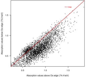
Figure 2.Raw absorption values above and below the Os absorp-tion edge for one soil aggregate slice from the synchrotron X-ray CT beamline.
resulting data and files as “diffedge” (difference at the ab-sorption edge). An example of the differences in abab-sorption values above (74.4 keV) and below (73.2 keV) the Os absorp-tion edge for one soil aggregate image slice example is shown in Fig. 2. Note that the absorption values are generally larger above the Os edge, i.e. below the 1 : 1 line in Fig. 2.
2.5.1 Creating masks for aggregate slices
Prior to analysing the synchrotron data at the three energy levels it was necessary to create masks of the aggregate out-lines so that pixels outside the aggregate could be excluded from the analysis. Where quartz beads (with similar density to soil material) occurred adjacent to aggregates in the syn-chrotron images, those pixels within the beads were replaced with background absorption values using the software pack-age VG Studio Max prior to creating masks for these im-ages. To create the masks we used a multistage procedure using scripts in the R environment and the image processing package Fiji (Schindelin et al., 2012), described in the sup-plementary material file.
Each mask was saved as an 8 bit .tif file. We wrote an R script using the raster package (Hijmans, 2014) to crop all the original images (nine aggregates each with two sets of images: (i) 53 keV and (ii) the diff edge images) using the masks for each associated image slice and setting all the val-ues outside the cropped region to a constant value.
2.5.2 Reduction of raster resolution
The original synchrotron image files comprised 2544×2544
that it was challenging to process these data using large 3-D numeric arrays, so we chose to reduce the resolution of the image stack by 50 % in each dimension. By doing so we achieved an 8-fold reduction (i.e. a 2-fold reduction in each dimension) in the size of the numeric array. Aggregation was carried out from top to bottom for each of two neighbour-ing layers (i.e. layers 1 and 2, 3 and 4, etc.). The aggregation process was carried out in three steps. All these steps were applied to the images from the 56 keV energy level and the diffedge files. First the masks were applied to each file and adjacent layers were aggregated horizontally (2-D) by a fac-tor of 2 using the aggregate function in the raster package (Hijmans, 2014) and using the mean function to compute the mean of the layers. Then the two horizontally aggregated lay-ers were averaged vertically yielding a matrix of dimension
1272×1272. Any averaged outlying values greater than 10
were set to a value of 10. The matrices were combined into a 3-D numeric array with the third (vertical dimension) equal to half the number of slices in the original data. These pro-cessing steps were undertaken using an MPI computer clus-ter.
2.5.3 Segmentation of solid and pore phases
An initial approach to segment solid and pore phases in each aggregate slice based on a two-component mixture algorithm was inconsistent with realistic assumed values for organic matter particle density (Rawlins et al., 2016). So we used (i) our measurements of total organic matter, (ii) the aggre-gate volume computed from the X-ray CT scans and (iii) as-sumed values for the mineral particle and organic matter den-sities to compute the proportion of pore space in each aggre-gate using the following approach.
We computed the mass of mineral matter (Mm) by
sub-tracting the mass of OM (Mom; 2×TOC content; Pribyl,
2010) from the total mass of the aggregate. We assume a
par-ticle density of the mineral parpar-ticles ofDmto be 2.65 g cm3
(Hall et al., 1977), so we calculated the volume of mineral material (Vm) in each aggregate as
Vm=
Mm
Dm
. (1)
We assume an OM density of 1.4 g cm−3 (Mayer et al.,
2004). We computed the volume of OM (cm−3) by dividing
the mass of OM by its density.
Vom=
Mom
Dom
(2)
In doing so we were able to determine the proportions of OM and mineral volumes in the solid phase, and the volume of
pore space (Vp) as the difference of their sum from the total
aggregate volume (Vag):
Vp=Vag−(Vom+Vm). (3)
For each aggregate we set the threshold greyscale value so that the total number of voxels assigned as pores equated to
Vp. We then created a series of .tif image files storing the
2-fold solid–pore classification, with a third class value for pixels outside the aggregate.
2.5.4 Porosity, surface area, pore diameter and tortuosity index
We used the images from the segmentation of solid and pore phases to compute a series of physical properties for each aggregate. Total porosity and surface area on planar/volume images were calculated using a bespoke Win32 computer program minkowski.exe that includes estimation algorithms published in Ohser and Mucklich (2000). The bespoke soft-ware was originally developed and verified by Alasdair Houston at SIMBIOS (Abertay University) as part of a re-search degree programme.
Pore diameters were computed using a combination of the BoneJ (Doube et al., 2010) plugin for Fiji and a bespoke program which uses the method of maximal inscribed balls (Ohser and Mucklich, 2000) to convert the BoneJ mask thick-ness map into pore diameters. We used the Fiji plugin Anal-yseSkeleton (Arganda-Carreras et al., 2010) to determine the tortuosity index (TI) of pore branches within each aggregate, computed as the length of the pore branch divided by the Eu-clidean distance between their furthest ends.
2.5.5 Separation of mineral and organic matter phases
To separate all the solid phase voxels into either mineral or OM classes, we used (i) the diffedge data values for each ag-gregate and (ii) the proportions of mineral and OM volumes in each aggregate. Those voxels with the largest values in the diffedge numeric array for each aggregate were assigned an OM classification, and the proportion of solid phase voxels assigned as OM was the volume proportion of OM in each aggregate (see Table 1). The other solid voxels were assigned a mineral classification. We reclassified the original mineral and pore classified arrays for each aggregate (Sect. 2.5.3) into a 3-fold classification (mineral, pore and OM).
2.6 Statistical and geostatistical analyses 2.6.1 Transition probabilities
then P(OM,pore)=P(pore|OM)P(OM), where the first con-ditional probability is the probability that a randomly se-lected neighbour of an OM voxel corresponds to pore space. We call it the transition probability from OM to pore. We use the transition probability between OM and pore as a quan-titative measure of OM accessibility. If one normalizes the respiration rate of an aggregate relative to its total organic content (effectively allowing for differences in P(OM) be-tween them), then it may be hypothesized that differences between the aggregates with respect to this response depend
on the transition probability P(pore|OM).
We computed transition probabilities for the 3-D numeric arrays in which each voxel was one of four classes: 0 – mineral (M); 1 – pore (pore); 2 – organic matter (OM); and 9 – mask. The total of the three transition probabilities
(P(pore|OM), P(M|OM) and P(OM|OM)) is 1. We wrote a
script in R that progressed from the from top to the bottom of the numeric array, starting from the second layer and end-ing at the penultimate layer. For every iteration three neigh-bouring layers were used (one above, a central layer, and one below), avoiding the outermost rows and columns of the 3-D array in the analysis. All three layers were simultane-ously shifted by one pixel around their initial position in the
x andy directions, while for every offset combination, the
voxel classification was queried and concatenated with the classification of the original non-shifted central layer which
shared the same spatial location (x andy). The class
com-parisons always originated from the central voxel to the
vox-els of the surrounding complete 3×3×3 array subset. For
the 26 neighbouring voxels, we considered transitions from the central OM voxels to the neighbouring 26 voxels. In ad-dition to the voxel class, we also recorded the direction of transition because (i) this was necessary to remove the com-bination where the central layer was compared with the non-shifted central layer and (ii) in future analyses (not in this pa-per) we may wish to undertake directional analyses of transi-tions. We computed the frequency of each class combination (transition) for each layer comparison, and in a final step the frequency of each transition and layer comparison was com-puted.
In a recent study, Falconer et al. (2015) used the propor-tion of OM-centred voxels which had at least one transipropor-tion to a pore voxel in adjacent voxels (in our case there were 26) as a measure of OM accessibility, and so we computed these proportions for our nine aggregates. To distinguish this addi-tional measure of accessibility from the transition probabili-ties, we refer to these former values as the minimum thresh-old OM–pore proportions.
2.6.2 Indicator variograms and variogram models
To understand the length scales over which the three phases vary, we computed 3-D indicator variograms (Webster and Oliver, 2007) for each phase and for each aggregate using scripts written in R with the gstat package (Pebesma, 2004).
Using the 3-D numeric arrays in which each voxel had been classified as either mineral, organic matter, pore or mask (ex-terior), we chose a random starting point within the numeric array of each aggregate and selected a cube of voxels with 200 voxels in each dimension around this point. We then checked that less than 10 % of the voxels were classed as mask. If mask values accounted for more than 10 % of all voxels, a new random starting point was selected until this condition was met. We converted this 3-D array into a gstat
object (x, y andzcoordinates plus the voxel class) and
ex-cluded the exterior voxels. To compute indicator variograms for each phase, we recoded the phase classes so that a sin-gle phase took a value of 1, and the other phases were set to 0. We then randomly selected a subset of 50 000 voxels with which to estimate the indicator semivariances for each phase at a series of increasing lag intervals up to a maximum of 250 voxels. We plotted a set of indicator variograms for each phase and fit a range of single authorized variogram models to them (Webster and Oliver, 2007) . In all cases the exponen-tial model gave the best fit and so we computed and recorded the parameters of the exponential model fitted to each set of indicator semivariances. For the model range parameter, we recorded the effective range, which in the gstat package is 3 times the theoretical range reported. We repeated this pro-cedure 50 times for each of the three phases in each of the nine aggregates to ensure that we encompassed the variation inside each aggregate. We note that each indicator variogram may not be independent because in some cases the starting points may be sufficiently close for the 3-D arrays of 200 units in each dimension to overlap.
3 Results and their interpretation
3.1 Aggregate properties and respiration rates
A set of properties determined for each of the nine soil ag-gregates is summarized in Table 1. There was an approxi-mately 2-fold variation in the quantity of TOC in the nine aggregates (range 4.18–7.7 %), whilst the magnitude of
res-piration (based on the CO2concentration scaled to the TOC
content) varies by more than a factor of 6 (range 10.5–
65.9 µg C mg C−1day−1). There was a positive correlation
between the magnitude SHR and TOC, with a Pearson
cor-relation ofr=0.29. We do not place too great an emphasis
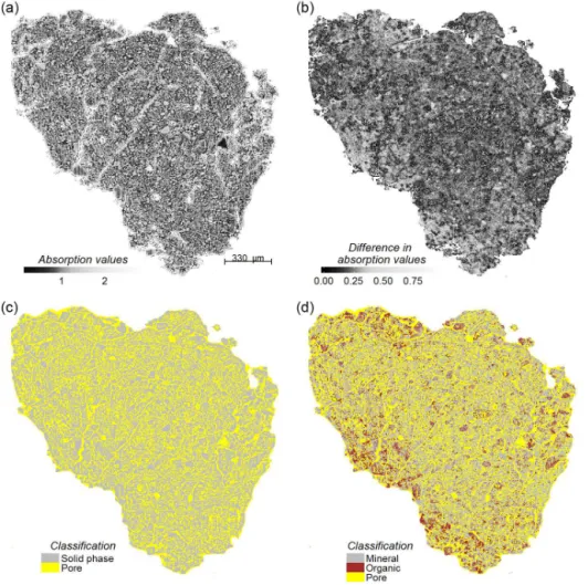
Figure 3.Horizontal cross section through one aggregate showing(a)the raw absorption values at the low energy (56 keV),(b)the difference in absorption between the two larger energy scans,(c)the distribution of solid and pore phases (determined usinga), and(d)the distribution of mineral, pore and organic matter determined using both(b)and(c).
between total porosity (based on averaging from the scan
res-olution of 3.3 µm) and bulk density (r= −0.98) for each of
the nine aggregates. There was a substantial, 4-fold variation in the surface area of the aggregates after it had been
nor-malized by aggregate volume (range 16.7–69.6 mm2mm−3;
see Table 1). The Pearson correlation between surface area normalized by aggregate volume and normalized headspace C gas concentration was both positive and reasonably large
(r=0.44), suggesting that the former may be a factor that
influences the latter.
Figure 3 shows the distribution of the OM, pore and min-eral phases in one aggregate slice. Using our approach to computing the volume of organic matter in each of the ag-gregates (Sect. 2.5.5), it exhibits a 2-fold variation between 10 and 19.5 %.
3.2 Pore diameters and tortuosity index values
Figure 4 shows how the pores of differing diameter (µm3)
contribute to the total pore space in each aggregate,
com-puted for the regular blocks extracted from each of the
aggre-gates. Pores with diameters of<22 and 22–30 µm3account
for the vast majority (82–89 %) of the total pore space in each aggregate. Aggregate 40 appears to be anomalous (Fig. 4), with a notably smaller porosity than the other aggregates. However, because this approach was applied to a subset of the aggregate volume (a regular three-dimensional region), in this case we believe it is not representative of the total ag-gregate pore space (a value of 30.7 % reported in Table 1) computed using the entire aggregate volume.
The total number of pore branches in each aggregate for which TI values were calculated for the nine aggregates ranged from 247 699 to 562 655. There is little variation in the overall distribution of TI values for the nine aggregates (Fig. 5), each having mean values between 1.29 and 1.31 and
each having a small number of more tortuous pores (TI>2),
Table 1.Physical properties of the nine soil aggregates and quantities of CO2released by the aggregates from soil heterotrophic respiration
during incubation (see text).
Aggregate number 37 40 43 49 55 61 67 73 76 Dry mass (mg) 106 118 177 103 112 177 146 101 103 Aggregate volume (mm3) 73.7 70.2 137.3 70.8 79.2 118.3 95.8 60.4 56.4 TOC (%) 6.81 5.27 7.06 5.53 7.7 6.63 6.83 4.18 7.48 Dry bulk density (g cm−3) 1.43 1.68 1.29 1.46 1.41 1.50 1.52 1.67 1.83 Porositya(%) 39.4 30.7 45.1 39.6 39.3 36.8 35.5 32.2 21.8 Mineral massb(mg) 91.2 105.5 152.2 91.7 94.8 153.8 125.9 92.6 87.7 OM volumec(%) 13.9 12.6 13.0 11.5 15.6 14.2 14.9 10.0 19.5 Mineral volumec(%) 46.7 56.7 41.8 48.9 45.2 49.0 49.6 57.8 58.7 Moisture loss (freeze-drying)d(%) 23.5 18.1 27.8 21.3 25.3 25.8 25.2 22.8 20.0 Surface areae(mm2) 3462 2085 2299 4929 4807 3895 4808 4037 2858 Surface area/agg. volume (mm2mm−3) 47.0 29.7 16.7 69.6 60.7 32.9 50.2 66.8 50.7 (Excess) headspace C concentrationf(mg kg−1) 76 108 238 350 223 477 656 127 301 Normalized C gas concentrationg(µg C mg C−1day−1) 10.5 17.3 19.1 61.5 25.8 40.6 65.9 30.1 39.0
aSolid–pore thresholds computed using aggregate volume and assumptions for organic matter and mineral particle density. This is an image-based porosity estimate based on averaging values at the scanning resolution of 6.6 µm.
bMineral mass computed from total aggregate mass – mass of organic matter (2×TOC).
cExpressed as a proportion of the solid volume (excludes pore space) and assumes a mineral density of 2.65 g cm−3.
dThe mass proportion (%) of moisture lost between mass of field-moist aggregates and freeze-dried mass (the latter after changes in moisture introduced through the pressure plate). We cannot compute volumetric moisture content (cm3cm−3) because the freeze-drying procedure also removes moisture from both pore space and organic matter. eSurface area was computed using a bespoke programme (see text).
fA background CO
2concentration of 400 mg kg−1was assumed.
gHeadspace C gas concentration normalized by the TOC content of each aggregate.
37 40 43 49 55 61 67 73 76
0.0 0.1 0.2 0.3 0.4
Aggregate volume fraction
Aggregate
Pore diameter / microns (1,22]
(22,30]
(30,43]
(43,60]
(60,72]
(72,85]
(85,97]
(97,110]
(110,125]
(125,137]
(137,150]
(150,165]
(165,250]
(250,400]
Figure 4.Distribution of pore diameters (µm3) expressed as a proportion of total volume of a regular 3-D region extracted from each of the nine aggregates.
with their magnitudes of respiration as we do not consider it would prove meaningful.
3.3 Transition probabilities
The transition probabilities from each organic-matter-centred voxel to the neighbouring 26 voxels for each of the nine ag-gregates is shown in Fig. 6, within a restricted region of a
ternary diagram. These transition probabilities are estimated for this voxel resolution (6.6 µm). We know that some vox-els may be misclassified because they represent a mixture of OM and mineral phases, and more accurate classifications may only be possible on finer scales.
Figure 5.Distribution of tortuosity index (dimensionless) for each of the nine aggregates.
phase (range 0.35–0.58). The range of organic to mineral phase transitions was between 0.32 and 0.49. In terms of OM accessibility, the OM–pore transition probabilities are gener-ally smaller (range 0.07–0.17) than transitions to the other two phases, indicating that a relatively small proportion of all OM voxels are accessible to soil microbes. The values of our alternative measure of OM accessibility, the proportion of OM-centred voxels with at least one adjacent pore voxel (the minimum threshold OM–pore proportions), are shown in Table 2. These values range from 0.13 to 0.19 % show-ing that the frequency distribution of the numbers of adja-cent pore voxels is positively skewed, with a larger frequency of voxels having only one OM–pore transitions compared to larger numbers of OM–pore transitions around a central OM
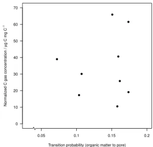
voxel. The Pearson linear correlation coefficient (r) between
the magnitude of SHR (rescaled to aggregate TOC content) and the transition probabilities from a central OM voxel to a neighbouring pore voxel was 0.12, which is not particularly strong (see Fig. 7).
3.4 Indicator variograms and models fitted to them
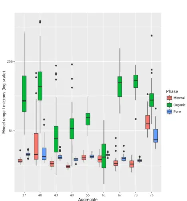
Figure 8 shows the variation of the effective range of the ex-ponential models fitted to the indicator variogram semivari-ance estimates for the 50 randomly selected blocks for the three phases in each of the aggregates. Selected statistics of the effective range values for OM are shown in Table 3.
With the exception of aggregate 61, the length scale (range value) over which organic matter varies is signifi-cantly greater than for both mineral and pore phases (Fig. 8) in all aggregates. In most cases the interquartile range for OM is generally large when compared to that of both
min-● ●
● ●
● ●
● ●
●
37 40
43
49
55 61
67 73
76
40 50 60 10
20
30
40 50 60
OM
OP
OO
OM
OP OO
Figure 6.Ternary diagram showing the overall transition probabili-ties (%) between a central organic matter voxel (side length 6.6 µm) and 26 adjacent voxels (see text) for each of the nine aggregates (la-belled). The transitions are between organic matter and each of the three phases (O: organic matter; P: pore; M: mineral). For example, OO is organic matter to organic matter. The truncated axes show only a sub-region of the ternary diagram. The osmium staining of OM sorbed onto mineral particles may have resulted in misclassifi-cation of voxels that are a mixture of OM and mineral matter. We cannot account for this because such effects could only be recon-ciled at finer (<6.6 µm) spatial resolutions.
●
● ●
●
● ● ●
● ●
Transition probability (organic matter to pore)
N
o
rm
a
liz
e
d
C
g
a
s
c
o
n
c
e
n
tr
a
ti
o
n
/
g
C
m
g
C
µ
−
1
0.05 0.1 0.15 0.2
0 10 20 30 40 50 60 70
Figure 7.Scatterplot showing the transition probabilities between a central voxel of organic matter and 26 neighbouring voxels versus the magnitude of respiration (normalized to aggregate TOC con-tent).
aggre-Table 2.The proportion of minimum threshold voxels (at least one OM-centred voxel has an interface with an adjacent pore voxel) in each soil aggregate.
Aggregate 37 40 43 49 55 61 67 73 76 Proportion (%) 0.16 0.17 0.13 0.16 0.14 0.15 0.15 0.19 0.14
Table 3. Selected statistics of the effective exponential model ranges (µm) fitted to the indicator variograms of organic matter vox-els for each of the nine aggregates.
25th 75th Aggregate percentile Median percentile SD 37 94 116 191 109 40 117 154 208 118
43 42 55 70 46
49 54 67 82 36
55 72 83 91 16
61 30 38 49 15
67 126 167 188 56 73 151 175 195 32 76 104 118 134 55
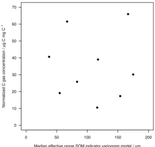
gates (median range value 38–175 µm3), we considered there
may also be equivalent differences in the frequency of mi-crosites for microbial respiration, with sites occurring more frequently where OM varies over shorter length scales. In Fig. 9 we show the median of the effective model ranges (Ta-ble 3) of OM matter plotted against the TOC normalized res-piration values from the laboratory measurements (Table 1). However, there is no linear relationship between these values
(Pearson linear correlation (r=0.01; Fig. 9).
We could not find other published studies which have re-ported the relative magnitude of unaccounted for short-scale (6.6 µm) variation of mineral, pore and OM phases in three dimensions within soil aggregates, and these values may be useful for similar studies. This unaccounted for variation (nugget variance) is the variance of analytical error plus vari-ation that occurs on scales shorter than the sampling reso-lution. The magnitude of nugget variance is often expressed as a proportion of the nugget plus sill variance (the variance at the range of the fitted model). Across all aggregates, the median proportions of nugget variance for the organic mat-ter phases varied between 0.47 and 0.73, whilst the range of the median proportions of the pore (0.0–0.09) and mineral (0.0–0.37) nugget variance were smaller.
4 Discussion
In our previous analysis (Rawlins et al., 2016), we reported what we now recognize were unrealistically small values for OM particle density, which gave rise to small total porosity values (4.4–11.1 %) in each aggregate. Using the modified approach we report here, there was a very strong correlation
● ● ● ●
●
● ●
● ●
●
● ● ●
● ●
● ●
● ● ● ●
● ● ● ● ● ●
● ●
●
● ● ● ● ●
●
● ●
● ●
●
● ● ●
●
64 256
37 40 43 49 55 61 67 73 76
Aggregate
Mo
d
e
l r
a
n
g
e
/
m
ic
ro
n
s
(
lo
g
s
c
a
le
)
Phase
Mineral
Organic
Pore
Figure 8.Box plot showing variations in the model range estimate for exponential models fitted to indicator variograms of the three phases (mineral, soil organic matter and pore space) for each of the nine aggregates. The semivariance estimates were computed from a subsample of 50 000 locations from 50 separate blocks (each mea-suring 200×200×200 voxels) within each aggregate.
(r= −0.98) between total soil porosity and aggregate bulk
density (BD) for our nine aggregates, which suggests that this approach was considerably more successful than the previous one.
● ● ●
●
● ●
●
● ●
0 50 100 150 200
Median effective range SOM indicator variogram model / µm
N
o
rm
a
liz
e
d
C
g
a
s
c
o
n
c
e
n
tr
a
ti
o
n
/
g
C
m
g
C
µ
−
1
0 10 20 30 40 50 60 70
Figure 9.Scatterplot of median model range estimate for exponen-tial models fitted to indicator variograms of organic matter versus headspace CO2gas concentration normalized to the carbon content
of the aggregate.
Our analyses could be used to improve quantitative
esti-mates of the accessibility of both particulate (>50 µm) and
finer OM in soil aggregates. Our analysis showed that OM voxels had an overall transition probability to a neighbour-ing pore voxel (our criteria of accessibility) of between 0.07 and 0.17. In their simulation study, Falconer et al. (2015) used proportions of accessible particulate OM voxels (those with at least one neighbouring pore voxel) of between 20 and 100 % (range of OM contents 1.4–7 %). Using the same metric, we estimated that accessible OM voxels account for a substantially smaller proportion (range 13–19 %) of the total quantity of OM in each of the nine aggregates. In their study Falconer et al. (2015) placed particulate organic matter (POM) at the pore–solid interface, which likely ac-counts for the larger particulate OM accessibility propor-tions they report, and this approach may require modifica-tion if more realistic OM accessibility propormodifica-tions are to be simulated. However, estimated organic matter to pore transi-tion probabilities may be larger at finer X-ray CT resolutransi-tions
(<6.6 µm), where any misclassification due to edge effects
can be resolved.
We plan to extend our analysis further using the approach proposed by Kravchenko et al. (2015) by (i) quantifying the distribution of particulate organic matter (length scales
>50 µm) and (ii) computing a statistic of pore connectivity
for each aggregate and plotting it against SHR, and (iii) iden-tifying those pores which are connected to the exterior of each aggregate, providing a direct pathway for the diffusion of gas to and from sites of intra-aggregate SHR. These data could be used to assess whether these factors are strongly correlated with the magnitude of SHR. It would also be help-ful to estimate the distribution of water-filled pores (Monga
et al., 2008) at the suction (−50 kPa) used in our experiment
as this would determine which sites of microbial respiration may have been anaerobic, influencing the magnitude of SHR. In subsequent work we will also attempt to determine the lo-cation of finely disseminated OM sorbed onto mineral sur-faces. In doing so we would need to identify an upper thresh-old size (volume and shape) for sorbed OM, and rules gov-erning the size and shape of neighbouring mineral particles.
We reported that for a set of nine aggregates there was some evidence that greater surface area of the solid phase (both mineral and organic matter phases) had a reasonably
strong positive correlation (r=0.44) with the magnitude
of SHR, having scaled the respiration rates to TOC con-tent. This relationship requires further investigation using macroaggregates with a wide range of TOC concentrations and textures to determine whether this relationship is statis-tically significant, and how it might be interpreted in relation to the frequency of the occurrence of microbial microsites.
In their study, Peth et al. (2014) used air-dried soil aggre-gates, whilst we chose to freeze-dry the aggregates in our experiment to maximize absorption of osmium onto organic carbon bonds. It would be useful to compare the results of both approaches to determine whether the drying process has significant implications for the extent of Os absorption throughout an aggregate. This could be achieved by com-paring the magnitude and spatial distribution of Os using energy-dispersive X-ray analysis linked to a scanning elec-tron microscope, the method used by Peth et al. (2014) to validate their original approach.
We chose to make a single measurement of SHR based
on the headspace concentration of CO2 after 24 h and this
will likely reflect mineralization of the most labile OM, the concentration of which will vary between aggregates. This may have been a dominant control on SHR, and we can-not account for it when we compare our measurements of SHR with the accessibility of OM in each aggregate. If sim-ilar studies are undertaken in future, it may be preferable to
make more frequent measurements of headspace CO2
con-centrations over a more prolonged period and to establish the quantities of more labile organic matter in each aggregate us-ing advanced analytical approaches (Sebag et al., 2006).
5 Conclusions
sim-ilar. After normalizing for aggregate volume, there was a 4-fold variation in the aggregate surface areas, and this had a
reasonably strong linear correlation (r=0.44) with the
mag-nitude of SHR (after scaling to TOC content). This relation-ship needs further investigation using a greater number of soil samples with a wider range of surface areas (soil tex-tures) and OM concentrations.
The transition probabilities between OM-centred voxels and adjacent pore voxels – a measure of OM accessibility – varied between 0.07 and 0.17 and were generally smaller than the transitions to the other two phases. We believe these are the first data to quantify 3-D macroaggregate OM ac-cessibility on fine scales and could be used to help param-eterize models of OM mineralization. There was a weak
lin-ear correlation (r=0.12) between OM accessibility
(transi-tion probability between pore and OM) and the magnitude of SHR. There were substantial differences in median length scales (median ranges 38–175 µm) over which OM varied between aggregates based on models fitted to their indica-tor variograms. Studies of the processes governing SHR in soil macroaggregates need to be undertaken on fine scales (less than 250 µm) because this is the upper threshold of the length scales over which mineral phases, pores and OM are likely to vary.
6 Data availability
The processed data, the large numeric arrays with classes for the three phases in each aggregate, are
available at
doi:10.5285/2eac5f6b-334c-44a9-bae0-87af5d1f828d. These arrays are stored using the
“ff” package format from the R environment: see https://cran.r-project.org/web/packages/ff/index.html.
There are four numeric values for each position in the 3-D arrays of each aggregate: 0 – mineral; 1 – pore; 2 – organic matter; 9 – mask (outside the aggregate).
To transfer the data to other formats, users will first need to import the data into R using the “ffload” function and ex-port them using their preferred format. It was not possible to provide the raw data because the datasets are prohibitively large (around 5 Tb).
The Supplement related to this article is available online at doi:10.5194/soil-2-659-2016-supplement.
Author contributions. The following authors made the speci-fied contributions to the paper: Barry G. Rawlins coordinated the project, lab work, data analysis and wrote parts of the manuscript; Christina Rheinhard and Robert C. Atwood undertook the syn-chrotron analyses of the osmium-stained soil aggregates and con-tributed to the synchrotron analyses in the manuscript; R. Mur-ray Lark contributed to the design of the experiment, the
geosta-tistical analysis of the data and wrote part of the manuscript; Alas-dair Houston provided the code for computing surface area and con-tributed to the manuscript. Joanna Wragg undertook the laboratory-based osmium staining and headspace CO2analyses and wrote the
methods section; Sebastian Rudolph wrote R codes for the analyses of transition probabilities of the 3-D arrays and other analyses and wrote the relevant section of the manuscript.
Acknowledgements. This work was supported by the use of the Diamond Beamline (I12) at the Diamond Synchrotron (Harwell, UK), project reference number EE9535. We thank Martin Hurst for helping to create the aggregate masks and Craig Sturrock for assistance with the image processing. We thank the following staff from BGS for their assistance with the beamtime at Diamond: Toni Milodowski, Jeremy Rushton, Lorraine Field and Dan Parkes. We thank Gemma Purser for undertaking the headspace CO2
analyses and Vicky Moss-Hayes for measuring the TOC content of the nine aggregates. Simona Hapca (Abertay University) devised the approach to create masks for each aggregate slice. This paper is published with the permission of the Executive Director of the British Geological Survey (NERC).
Edited by: S. Sleutel
Reviewed by: two anonymous referees
References
Arganda-Carreras, I., Fernández-González, R., Muñoz-Barrutia, A., and Ortiz-De-Solorzano, C.: 3D reconstruction of histological sections: Application to mammary gland tissue, Microsc. Res. Techniq., 73, 1019–1029, doi:10.1002/jemt.20829, 2010. Chenu, C., Hassink, J., and Bloem, J.: Short-term changes in the
spatial distribution of microorganisms in soil aggregates as af-fected by glucose addition, Biol. Fert. Soil., 34, 349–356, 2001. Cox, P., Betts, R., Jones, C., Spall, S., and Totterdell, I.:
Accelera-tion of global warming due to carbon-cycle feedbacks in a cou-pled climate model, Nature, 408, 184–187, 2000.
Davidson, E. and Janssens, I.: Temperature sensitivity of soil carbon decomposition and feedbacks to climate change, Nature, 440, 165–173, doi:10.1038/nature04514, 2006.
Doube, M., Kłosowski, M. M., Arganda-Carreras, I., Cordelières, F. P., Dougherty, R. P., Jackson, J. S., Schmid, B., Hutchin-son, J. R., and Shefelbine, S. J.: BoneJ: Free and extensi-ble bone image analysis in ImageJ, Bone, 47, 1076–1079, doi:10.1016/j.bone.2010.08.023, 2010.
Dungait, J. A. J., Hopkins, D. W., Gregory, A. S., and Whit-more, A. P.: Soil organic matter turnover is governed by acces-sibility not recalcitrance, Glob. Change Biol., 18, 1781–1796, doi:10.1111/j.1365-2486.2012.02665.x, 2012.
Falconer, R. E., Battaia, G., Schmidt, S., Baveye, P., Chenu, C., and Otten, W.: Microscale Heterogeneity Explains Experimental Variability and Non-Linearity in Soil Or-ganic Matter Mineralisation, PLoS ONE, 10, e0123774, doi:10.1371/journal.pone.0123774, 2015.
Monograph No. 9, Rothamsted Experimental Station, Harpen-den, 1–75, 1977.
Hapca, S., Baveye, P. C., Wilson, C., Lark, R. M., and Ot-ten, W.: Three-Dimensional Mapping of Soil Chemical Char-acteristics at Micrometric Scale by Combining 2D SEM-EDX Data and 3D X-Ray CT Images, PLOS ONE, 10, 1–17, doi:10.1371/journal.pone.0137205, 2015.
Hijmans, R. J.: raster: Geographic data analysis and modeling, http://CRAN.R-project.org/package=raster (last access: 21 Oc-tober 2016), r package version 2.3-0, 2014.
Hirano, T., Kim, H., and Tanaka, Y.: Long-term half-hourly mea-surement of soil CO2concentration and soil respiration in a
tem-perate deciduous forest, J. Geophys. Res.-Atmos., 108, 4631, doi:10.1029/2003JD003766, 2003.
Hodgson, J. M.: Soil Survey Field Handbook, Technical Mono-graph No. 5, Rothamsted Experimental Station, Harpenden, 1– 86, 1974.
Juarez, S., Nunan, N., Duday, A.-C., Pouteau, V., Schmidt, S., Hapca, S., Falconer, R., Otten, W., and Chenu, C.: Ef-fects of different soil structures on the decomposition of na-tive and added organic carbon, Eur. J. Soil Biol., 58, 81–90, doi:10.1016/j.ejsobi.2013.06.005, 2013.
Killham, K., Amato, M., and Ladd, J.: Effect of substrate loca-tion in soil and soil pore-water regime on carbon turnover, Soil Biol. Biochem., 25, 57–62, doi:10.1016/0038-0717(93)90241-3, 1993.
Kravchenko, A. N., Negassa, W. C., Guber, A. K., and Rivers, M. L.: Protection of soil carbon within macro-aggregates depends on intra-aggregate pore characteristics, Scientific Reports, 5, 16261, doi:10.1038/srep16261, 2015.
Lark, R. M., Rawlins, B. G., Robinson, D. A., Lebron, I., and Tye, A. M.: Implications of short-range spatial variation of soil bulk density for adequate field-sampling protocols: methodology and results from two contrasting soils, Eur. J. Soil Sci., 65, 803–814, doi:10.1111/ejss.12178, 2014.
Lehmann, J., Kinyangi, J., and Solomon, D.: Organic matter sta-bilization in soil microaggregates: implications from spatial het-erogeneity of organic carbon contents and carbon forms, Biogeo-chemistry, 85, 45–57, doi:10.1007/s10533-007-9105-3, 2007. Leue, M., Ellerbrock, R. H., and Gerke, H. H.: DRIFT mapping of
organic matter composition at intact soil aggregate surfaces (in Preferential flow), Vadose Zone J., 9, 317–324, 2010.
Li, Y., Liu, Y., Wu, S., Niu, L., and Tian, Y.: Microbial prop-erties explain temporal variation in soil respiration in a grass-land subjected to nitrogen addition, Scientific Reports, 5, 18496, doi:10.1038/srep18496, 2015.
Mayer, L. M., Schick, L. L., Hardy, K. R., Wagai, R., and McCarthy, J.: Organic matter in small mesopores in sedi-ments and soils, Geochim. Cosmochim. Ac., 68, 3863–3872, doi:10.1016/j.gca.2004.03.019, 2004.
Monga, O., Bousso, M., Garnier, P., and Pot, V.: 3D geometric struc-tures and biological activity: Application to microbial soil or-ganic matter decomposition in pore space, Ecol. Model., 216, 291–302, doi:10.1016/j.ecolmodel.2008.04.015, 2008.
Moyano, F. E., Vasilyeva, N., Bouckaert, L., Cook, F., Craine, J., Curiel Yuste, J., Don, A., Epron, D., Formanek, P., Franzlueb-bers, A., Ilstedt, U., Kätterer, T., Orchard, V., Reichstein, M., Rey, A., Ruamps, L., Subke, J.-A., Thomsen, I. K., and Chenu, C.: The moisture response of soil heterotrophic respiration:
in-teraction with soil properties, Biogeosciences, 9, 1173–1182, doi:10.5194/bg-9-1173-2012, 2012.
Negassa, W. C., Guber, A. K., Kravchenko, A. N., Marsh, T. L., Hildebrandt, B., and Rivers, M. L.: Properties of Soil Pore Space Regulate Pathways of Plant Residue Decomposition and Community Structure of Associated Bacteria, PLOS ONE, 10, e0123999, doi:10.1371/journal.pone.0123999, 2015.
Ohser, J. and Mucklich, F.: Statistical Analysis of Microstructures in Materials Science, John Wiley & Sons, 404 pp., 2000. Pebesma, E. J.: Multivariable geostatistics in S: the gstat package,
Comput. Geosci., 30, 683–691, 2004.
Peth, S., Chenu, C., Leblond, N., Mordhorst, A., Garnier, P., Nunan, N., Pot, V., Ogurreck, M., and Beckmann, F.: Localiza-tion of soil organic matter in soil aggregates using synchrotron-based X-ray microtomography, Soil Biol. Biochem., 78, 189– 194, doi:10.1016/j.soilbio.2014.07.024, 2014.
Pribyl, D. W.: A critical review of the conventional {SOC} to {SOM} conversion factor, Geoderma, 156, 75–83, doi:10.1016/j.geoderma.2010.02.003, 2010.
R Core Team: R: A Language and Environment for Statistical Com-puting, R Foundation for Statistical ComCom-puting, Vienna, Austria, http://www.R-project.org/ (last access: 21 October 2016), 2013. Rawlins, B. G., Wragg, J., Rheinhard, C., Atwood, R. C.,
Hous-ton, A., Lark, R. M., and Rudolph, S.: Three dimensional soil organic matter distribution, accessibility and microbial respira-tion in macro-aggregates using osmium staining and synchrotron X-ray CT, SOIL Discuss., doi:10.5194/soil-2016-32, in review, 2016.
Schindelin, J., Arganda-Carreras, I., Frise, E., Kaynig, V., Longair, M., Pietzsch, T., Preibisch, S., Rueden, C., Saalfeld, S., Schmid, B., Tinevez, J. Y., White, D. J., Hartenstein, V., Eliceiri, K., Tomancak, P., and Cardona, A.: Fiji: an open-source platform for biological-image analysis, Nat. Methods, 9, 676–682, 2012. Sebag, D., Disnar, J. R., Guillet, B., Di Giovanni, C., Verrecchia,
E. P., and Durand, A.: Monitoring organic matter dynamics in soil profiles by “Rock-Eval pyrolysis”: bulk characterization and quantification of degradation, Eur. J. Soil Sci., 57, 344–355, doi:10.1111/j.1365-2389.2005.00745.x, 2006.
Tisdall, J. M. and Oades, J. M.: Organic matter and water-stable aggregates in soils, J. Soil Sci., 33, 141–163, doi:10.1111/j.1365-2389.1982.tb01755.x, 1982.
Webster, R. and Oliver, M. A.: Geostatistics for Environmental Sci-entists, Second Edition, John Wiley and Sons, Ltd, Chichester, 330 pp., 2007.
World Reference Base 2006: World Reference Base for Soil Re-sources 2006, World Soil ReRe-sources Reports No. 103, FAO Rome, Rome, 145 pp., 2007.