UFMG – FEDERAL UNIVERSITY OF MINAS GERAIS Post-Graduation Program on Metallurgical and Mining Engineering
Doctoral Thesis
“Prediction and control of geometric distortion and residual stresses in hot
rolled and heat treated large rings”
Author: Alisson Duarte da Silva Advisor: Paulo Roberto Cetlin
UFMG – FEDERAL UNIVERSITY OF MINAS GERAIS Post-Graduation Program on Metallurgical and Mining Engineering
Alisson Duarte da Silva
PREDICTION AND CONTROL OF GEOMETRIC DISTORTION AND RESIDUAL STRESSES IN HOT
ROLLED AND HEAT TREATED LARGE RINGS
Doctoral Thesis presented to the Post-Graduation Program on Metallurgical and Mining Engineering at Federal University of Minas Gerais.
Area of concentration: Metallurgy of Transformation Advisor: Paulo Roberto Cetlin
Belo Horizonte
iii ACKNOWLEDGEMENTS:
The author of this work would like to thank all people who helped directly or indirectly towards the completion of this thesis, and in special:
My advisor Dr. Paulo Roberto Cetlin. This research work would not have been possible if not for his trust, efforts and guidance under technical and philosophic aspects.
My co-advisor Dr. Taylan Altan, who has given to me the opportunity of developing this work at ERC/NSM (Engineering Research Center/Net Shape Manufacturing) at The Ohio State University, making possible the cooperative work between UFMG and ERC/NSM.
Tércio A. Pedrosa, Jose L. Gonzalez-Mendes, and Xiaohui Jiang, for all their efforts as part of the group which has worked with me in this project. Sincere thanks are extended to all the students and staff of the Mechanical Forming Laboratory at UFMG and ERC/NSM at The Ohio State University.
SFTC (Scientific Forming Technologies, USA) and Chris Fischer, Research Engineer at SFTC, for establishing the first contact between UFMG and ERC/NSM and for the assistance in the simulations development.
FIA (Forging Industry Association), FIERF (Forging Industry Education and Research Foundation), and Carola Sekreter, Technical Director at FIA, for their trust and financial support.
CAPES (Coordination for the Improvement of Higher Education Personnel), for the Ph.D. scholarship and financial support to the project.
iv FAPEMIG (Foundation for the Support of Research in the Minas Gerais State), for the financial support to the project.
Sente Software Ltd., UK for providing AISI 4140 material data, based on JMatPro, for the simulation.
v TABLE OF CONTENTS:
1. INTRODUCTION ... 1
2. OBJECTIVES ... 6
3. LITERATURE REVIEW ... 8
3.1. Metal Forming ... 8
3.1.1. Historical Background ... 8
3.1.2. Definition and Classification ... 9
3.2. Heat Treatment of Steel ... 12
3.2.1. Definition ... 12
3.2.2. TTT and CCT Diagrams ... 15
3.2.3. Normalizing ... 18
3.2.4. Quenching ... 21
3.2.5. Hardenability ... 23
3.3. Stress ... 26
3.3.1. Principal Stress ... 26
3.3.2. Effective Stress ... 28
3.3.3. Residual Stress ... 31
3.4. Strain ... 35
3.4.1. Definition ... 35
3.4.2. Elastic, Plastic and Thermal Strain ... 36
3.4.3. Phase Transformation and Transformation Plasticity Strain ... 38
3.5. Stress-Strain Curves ... 40
3.5.1. The Tension Test ... 40
3.5.2. Determining the True Stress-Strain Curve with Yield and Ultimate Tensile Strengths ... 43
3.6. Interface Conditions between Workpiece and Environment ... 44
3.6.1. Heat Transfer during Air Cooling ... 44
3.6.2. Radiation Exchange between Surfaces ... 46
3.6.3. Heat Transfer during Quenching Process ... 48
vi
3.7. Heat Treatment Distortion ... 55
3.7.1. Mechanisms of Distortion ... 55
3.7.2. Quench Distortion ... 58
3.7.3. Test for Evaluating Quench Distortion (Navy C-Ring) ... 64
3.8. Rolled Rings ... 71
3.8.1. Application ... 71
3.8.2. Forming of Rings ... 72
3.8.3. Heat Treatment of Hot Rolled Rings ... 74
3.8.4. Heat Treatment Distortion of Rings ... 75
3.8.5. Correction of Ring Ovality (Circumferential Distortion) ... 78
3.9. AISI 4140 Steel ... 80
3.9.1. Characteristics and Properties ... 80
3.9.2. Material Phases ... 84
3.10. Finite Element Method ... 89
3.10.1. Historical Background and Application ... 89
3.10.2. Metal Forming Simulation ... 92
3.10.3. Heat Treatment Simulation ... 97
4. METHODOLOGY ... 101
4.1. Validation of the Heat Treatment Simulation Methodology using a Navy C-Ring Test ... 101
4.1.1. Experimental test ... 101
4.1.2. Numerical Simulation ... 103
4.2. Prediction of Ring Distortion during Heat Treatment Processes ... 106
4.2.1. Numerical Simulation of Normalizing ... 106
4.2.2. Numerical Simulation of Quenching ... 108
4.3. Correction of Distortion ... 111
5. RESULTS AND DISCUSSION ... 116
5.1. The Validation of Heat Treatment Simulation using a Navy C-Ring Test .... 116
5.1.1. Experimental Test ... 116
5.1.2. Numerical Simulation ... 118
vii
5.2.1. Normalizing of Hot Rolled Rings ... 124
5.2.2. Quenching of Hot Rolled Rings ... 126
5.3. Correction of Ring Distortion ... 131
6. SUMMARY AND CONCLUSION ... 137
7. ORIGINAL CONTRIBUTIONS TO KNOWLEDGE ... 139
8. RELEVANCE OF THE RESULTS ... 140
9. FUTURE WORK ... 141
viii LIST OF FIGURES
Figure 3.1 – The C equilibrium diagram up to 6.67 wt% C. Solid lines indicate Fe-Fe3C diagram; dashed lines indicate iron-graphite diagram (Ericsson, 1991). ... 13
Figure 3.2 – Diagram showing how measurements of isothermal transformation are summarized by the isothermal transformation diagram (Voort, 1991). ... 16 Figure 3.3 – Schematic chart illustrating relationship of (a) quench and temper type of hardening treatment and (b) conventional annealing cycle to a typical TTT diagram (Voort, 1991). ... 17 Figure 3.4 – Correlation of CCT and TTT diagrams with end-quench hardenability test data for 4140 steel (Voort, 1991). ... 18 Figure 3.5 – Partial iron-iron carbide phase diagram showing typical normalizing range for plain carbon steels (Ericsson, 1991). ... 19 Figure 3.6 – Comparison of time-temperature cycles for normalizing and full annealing. The slower cooling of annealing results in higher temperature transformation to ferrite and pearlite and coarser microstructures than does normalizing (Kraus, 1980). ... 20 Figure 3.7 – Effect of normalizing on the grain structure in steels; (a) structure of as-hot rolled steel, and (b) the same steel after normalizing (Sharma, 1996). ... 20 Figure 3.8 - Microstructure evolution in a 4140 steel during cooling at (a) 20°C/s and (b) 5°C/s (Guo et al., 2009). ... 21 Figure 3.9 – Typical (a) plate and (b) lath martensite (Krauss and Marder, 1971). ... 23 Figure 3.11 - Microstructure change along the Jominy quench bar for (a) 4140, and (b) 5140 alloys (Guo et al., 2009). ... 25 Figure 3.12 – Experimentally determined CCT diagram (solid lines) for AISI 4140. TTT diagram (dashed lines) is also shown (Totten et al., 1993). ... 25 Figure 3.13 – Schematic representation of extend of hardening in oil-quenched and water-quenched bars of SAE 3140 steel of various diameters. The cross-hatched areas represent the unhardened core (Grossmann and Bain, 1964). ... 26 Figure 3.14 – Stress acting on an element. (a) Cylinder upsetting process. (b) Forces acting on an element. (c) Stress components acting on an element (Altan et al., 2005). 27
x Figure 3.30 – Two rings exchanging heat with the environment (modified from Incropera et al., 2007). ... 47 Figure 3.31 - Cooling curve and cooling rate curve at the center of a 25 mm diameter stainless probe quenched with 95 °C water flowing at 15 m/min (Bates et al., 1991). .. 49 Figure 3.32 – Series of photographs illustrating the various stages in the quenching process using normal speed quenching oil (Houghton, 2011). ... 49 Figure 3.34 – Heat transfer coefficient versus surface temperature of an austenitic steel cylinder (25-mm diameter x 100mm) quenched into water at 30°C and into a fast oil at 60°C flowing at 0.3 m/s (Totten, 2007). ... 51 Figure 3.35 – Variation in the heat transfer coefficient around the bar for transverse flow with (a) no agitation and (b) agitation (Sedighi and McMahom, 2000). ... 52 Figure 3.36 – (a) Surface thermocouples used on an instrumented high-pressure turbine disk to establish HTC (Schirra and Goetisshius, 1992; in Wallis, 2010). ... 53 Figure 3.37 – A flow chart for iterative determination of HTC (Xiao et al., 2010). ... 54 Figure 3.38 – Case study of the determination of heat transfer coefficient during quenching of an aluminum casting part: (a) thermocouples locations; (b) measuring cooling curves; and (c) interactively determined HTC (Xiao et al., 2010). ... 54 Figure 3.39 – Heat transfer coefficients around a ring cooled in oil (Segerberg and Bodin, 1992; in Wallis, 2010). ... 55 Figure 3.40 – Definition of distortion (Li et al., 2006). ... 56 Figure 3.41 – Coupling effects among quenching characteristics (Totten and Howes, 1997). ... 57 Figure 3.42 – Schematic representation of various couplings between physical fields (Nallathambi et al., 2010). ... 59 Figure 3.43 – Boiling behavior and distortion during quenching in still city water at 30°C (Arimoto et al., 1998; in Narazaki et al., 2002). ... 59 Figure 3.44 - Distortion response for notched bars; distortion magnified 10x (Freborg et al., 2007). ... 60
xii Figure 3.59 – Simulated dimensional displacement in the x-direction for all cases from start of heating through end of quench. Results are given at nodal locations “B” at the
gap, and local at node “C” on the outside diameter (Hardin and Beckermann, 2005). .. 68
Figure 3.60 – Simulated martensite volume fraction for the 4140 alloy cases, from start of heating through end of quench. Results are given at nodal locations “A” at the center of the piece, “B” at the gap, and local at node “C” on the outside diameter (Hardin and Beckermann, 2005). ... 69
Figure 3.61 – (a) Model of a c-ring: system for (b) vertical and (c) side immersion (Brooks and Beckermann, 2007). ... 70
Figure 3.62 – Method for identifying distortions (Cyril et al., 2009). ... 70
Figure 3.63 – C-ring distortions after heat treatment (Cyril et al., 2009). ... 70
Figure 3.64 – Blank preparation for ring rolling process; (a) open-die and (b) pot-die operations (Gellhaus 2011). ... 72
Figure 3.65 – Radial-axial ring rolling process (Gellhaus, 2011). ... 73
Figure 3.66 – Typical range of rings during ring rolling process (Brümmer, 2011). ... 73
Figure 3.67 – Most common processes used for rings after ring rolling stage. ... 74
Figure 3.68 – Rings in stacks during heating process; (a) rings prepared for heating and (b) after heating (McINNES Rolled Rings, 2011). ... 75
Figure 3.69 – Tanks for quenching of hot rolled rings (Rotek® Rings, 2011)... 75
Figure 3.70 – Distortion of two different ring sections; (a) Thin-walled ring and (b) thick-walled ring; displacement is magnified 10x (Pascon et al., 2004). ... 76
Figure 3.71 – Material phases percentage after quenching of AISI 4140 steel rings (scale: black color = 100%); (a) phases distribution in the tall and thin ring (without .. 76
Figure 3.72 – Typical arrangement of ring stacks in the quenching tank. ... 77
Figure 3.73 – Ring ovality caused by an inadequate hot rolling process (Buhl, 2011). . 78
Figure 3.74 – Schematic of systems used to correct ring ovality; (a) an expander and (b) a compresser. ... 79
Figure . – Hardenability diagram of 4140 . ... 82
xvii LIST OF TABLES
Table 3.1 – Classification of massive forming processes (Altan et al., 1983). ... 11
Table 3.2 – Classification of sheet metal forming processes (Altan et al., 1983). ... 11
Table 3.6 – AISI 4140 chemistry (ASM International, 1993). ... 80
Table 3.7 – AISI 4140 cross-reference (ASM International, 1993). ... 80
Table . – Typical Mechanical Properties of AISI 4140 . ... 82
Table 4.1 – Nominal composition of AISI 4140 steel (in wt%). ... 102
Table 4.5 – FE setup for the simulation of quenching process. ... 115
Table 5.1 – Measured hardness after oil quenching process. ... 117
xviii ABSTRACT
xix RESUMO
1 1. INTRODUCTION
The global scenario of the manufacturing industry is guided by a high level of market competition. New technologies and innovative ideas are part of the companies’ strategies to maintain its products with a good relation between costs and benefits, improve its market share, and attend to the customer’s specifications.
Following the same tendency, metal forming industry demands the use of computational technologies applied to Engineering. One typical application is the simulation of manufacturing processes using CAE (Computer Aided Engineering) technology, with the objective of tooling design and manufacturing optimization, saving project time and costs. CAE technology has become essential for metal forming processes, being implemented in the material flow analysis and optimization, and in the die stress analysis. Moreover, the design is developed in shorter periods of time, when compared to the development without computational tools, and experimental tests may be conducted resulting in more assertive process objectives and predictions.
The experimental validation is an essential stage of a metal forming process study. However, this is not a trivial procedure. Its success depends on the correct and methodic conduction of the simulation stage. CAE tools are nothing else than powerful computational tools, and their use should be based on a strong technical background. The model based on the Finite Element Method (FEM) should be correctly set and the results analyzed and criticized, improving the model when necessary. In addition, mechanical machines and tools used for experimental stage are expensive, and are usually defined for new projects, demanding time and investments. The complexity and cost of metal forming facilities increases even more when geometric tolerances are critical issues. Therefore, a complete manufacturing process characterization should consider a financial viability analysis.
2 which is plastically deformed through one or more operations towards a relative complex geometry. The near net shape manufacturing, or net shape, drastically reduces the material removal, saving material and energy. Usually, metal forming requires expensive tooling, so the process is economically attractive when a large number of parts has to be produced or the required mechanical properties of the final product can only be obtained through forming process.
Constant increase of material and energy, and tendency to obtain flexible manufacturing systems, requires that metal forming processes de designed with a minimum number of trial and error. For this reason, CAD/CAM (Computer Aided Design/Computer Aided Manufacturing) and also CAE technologies are tools with a large acceptance in the metal forming field. The practical use of these techniques requires a thorough knowledge of the principal variables of a metal forming process and their interactions. Altan et al. (1983) include in these variables: the flow behavior of the formed material and the processing conditions; tooling geometry and materials; friction; the mechanics of deformation; the characteristics of the forming equipment; the product geometry, tolerances, surface finishing and mechanical properties, and the effect of the process on the environment.
Seamless rings are an example of parts that are produced using a near net shape metal forming process called ring rolling. Usually, a simple geometry as a billet is heated, upset, backward extruded, and pierced. Then the initial ring is hot rolled to obtain large diameters. This process has been developed by trial and error methodology. However, advanced 3D simulations have been developed in the last years to optimize this process. Despite the advance in computer technology, computation of a complete ring rolling model is still tremendously time consuming. The complexity of the process creates the necessity of special modules in simulation software exclusive for ring rolling practice. But CAE tools have evolved and this process has been better investigated and optimized (Wang et al., 2010).
3 However, the 3D simulation has been widely implemented in the industry for metal forming design. The evolution of computational processing has increased computers efficiency, providing faster systems that can solve equations used in the FEM.
More recently, FEM software packages have been developed for thermomechanical and heat treatment processes emulating capability. The level of the complexity to simulate it increases considerably, when compared to more simple forming simulations. New models and material data are necessary. Grain growth and phase transformation are some examples of processes occurring during simulations. Material phases have to be taken in account, each one with its thermophysical and mechanical properties, and the transformation kinetics has to be established. As a result, FEM equations become more elaborated.
Heat treating is defined as heating and cooling a solid metal or alloy in such a way as to obtain desired conditions or properties (ASM International, 1995). Some of the objectives of heat treating metal and alloy parts include: removing of stresses, refinement of the grains structure, increase hardness, increase thoughness, and change magnetic properties. Heat treatment commonly involves a quenching step, which may cause undesired geometrical distortions in the processed parts. The dimensional accuracy of these parts is affected and leads to production and economical losses. In these cases, the heat treatment process should be optimized, avoiding these distortions, usually caused by fast cooling. FEM simulations can be used to predict the quenching process, predicting defects such as distortions, and be used to improve the process by improving the FE model parameters. However, for certain situations, a mechanical process after heat treatment is necessary due to the impossibility of preventing defects or financial reasons.
4 rotation of the ring section (Pascon et al., 2004). In many situations, the cooling conditions can be better controlled and distortions may be avoided.
In special, hot rolled ring industry has reported a circumferential distortion in large rings after quenching process. Rings with relatively large diameter and thin thickness may lead to an out-of-roundness shape during fast cooling processes. These rings are quenched in tanks, disposed in stacks with more than one ring each stack. Due to the high production rate necessity, many rings are quenched at the same time, in the same quenching tank. Several parameters influence the quenching process, including: quenchant temperature, polymer concentration, bacteria quantity, and velocity (agitation inside the tank), and rings size and position inside the tank. Due to the described parameter, for the same ring, there is always a non-homogeneous heat transfer between ring and environment along the ring surface.
Forging industry and tank design companies have tried to develop more efficient systems, creating conditions during quenching where the ring may reach a symmetric heat transfer with the environment. For certain products, in special small geometries and/or lower production rate, the tank conditions may be better controlled, resulting in quenched parts without distortion. However, for large geometries inside large tanks, forging industry has concluded that it is impossible or not practical to avoid circumferential distortions. Some of the rings will always reach an out-of-roundness shape.
There is a wide variety of rings. Materials used for the rings include aluminum, titanium, magnesium, steel and nickel based specialty alloys. As an example, steel alloy rings have a minimum market price of 5 thousand dollars, and some inconel rings might cost 60 thousand dollars. The high value-added to these products creates the necessity of correcting the out-of-roundness shape of the rings, in order to satisfy the tolerances to ship to the costumers.
5 expanders pull the ring, involving small plastic deformations, reaching a near round shape. However, these are very sophisticated machines, which may cost up to 6 million dollars. In addition, the learning curve for these equipments is long and expensive.
Alternatively, hot rolled ring companies have developed simpler systems in order to correct the out-of-roundness shape of the rings. Compressive machines using flat tools are used to compress the ring, creating small plastic deformation, and correcting the circumference. However, this process is totally based on trial and error methodology, conducted based on operator experiences. Long times are used during this process. Some distortions and/or mistaken procedures can over deform the ring, and the product becomes scrap.
In addition, the rings display residual stresses after quenching process. These residual stresses decrease after tempering stage. However, some residual stresses still remain in the ring. Depending on the residual stresses magnitudes, the ring may distort during subsequent machining process. The mechanical procedure to correct the quench distortion may also decrease the residual stresses in the ring.
Finally, it is necessary to define a methodology to predict circumferential distortion of rings due to heat treatment processes. Once the out-of-roundness ring is obtained, it is possible to develop a procedure to correct the distortion through small plastic deformations.
6 2. OBJECTIVES
As introduced in the previous section, distortions of hot rolled and heat treated rings are an important issue for the product quality. This work proposes to define a methodology to predict and correct geometric distortion and residual stresses of hot rolled and heat treated rings. This methodology will be based on FE simulations, using DEFORM-3DTM. An AISI 4140 ring case study will be used for this project investigation. The objective can be divided in 3 main tasks, each one with its specific approaches:
Objective 1: define a methodology to simulate heat treatment distortion using FE simulation. The following approaches should be investigated:
Conduct experimental oil quenching process using AISI 4140 navy c-ring specimens.
Investigate AISI 4140 material data for heat treatment simulation, considering its phases and the transformation kinetics between them.
Simulate oil quenching of AISI 4140 navy c-ring specimens.
Validate the heat treatment simulation comparing predicted and experimental results for distortion, martensite volume fraction, and hardness.
Objective 2: develop a methodology to obtain circumferential distortion of large rings, investigating predefined heat treatment stages, based on the procedure performed and validated for Objective 1. An AISI 4140 ring should be used as a case study. The stages to be investigated should approach as follows:
Investigate is the possibility to obtain circumferential distortion during normalizing process due to the proximity between two rings disposed 10 mm distant from each other in the cooling stage.
Establish a methodology to predict circumferential distortion during quenching of large rings.
Verify the residual stresses of the distorted ring after quenching process.
7
Propose an experimental methodology to be conducted at the shop floor.
Perform a distortion correction case study using FE simulation.
8 3. LITERATURE REVIEW
3.1. Metal Forming
3.1.1. Historical Background
Metalworking is probably the earliest technological occupation known to mankind; native metals must have been forged and shaped more than 7,000 years ago (Schey, 1970). The earliest records of metalworking describe the simple hammering of gold and copper in various regions of the Middle East around 8000 B.C. The forming of these metals was crude because the art of refining by smelting was unknown and because the ability to work the material was limited by impurities that remained after the metal had been separated from the ore.
Around 400 B.C. the smelting of the copper was developed, and the metals purifying methodology began to be created. Later, it was observed that hammering metals increased its strength bu plastic deformation steps (strain hardening). Most metalworking was done by hand until the 13th century. At this time, the tilt hammer was developed and used primarily for forging bars and plates. Leonardo da Vinci’s notebook includes a sketch of a machine designed in 1480 for the rolling of lead for stained glass windows. In 1495, da Vinci is reported to have rolled flat sheets of precious metal on a hand-operated two-roll mill for coin making purposes (Semiatin, 2005). The 17th century saw the appearance of the slitting mills in which forged flats were split with collared rolls, then rounded by forging and finally drawn into wire. Grooved rolls were also used in France.
9 3.1.2. Definition and Classification
Metals exhibit a ductile behavior and respond elastically if stress is kept within a certain region, variously referred to as elastic region, elastic range or elastic domain. Beyond that region, plastic deformation takes place (Pagliettt, 2007). The use and control of the plastic deformation region (and also elastic) in metals is applied to manufacturing processes to obtain a wide variety of metal shapes. This practice can be understood as metal forming.
Metal forming is the group of deformation processes in which a metal billet or blank is shaped by tools or dies. According to Altan (1999), in metal forming, the starting material has a relatively simple geometry; this material is plastically deformed in one or more operations into a product of relative complex configuration. Forming to near net or to near net shape dimensions drastically reduces metal removal requirements, resulting in significant material and energy savings. Metal forming includes processes such as rolling, extrusion, cold and hot forging, bending, and deep drawing.
The design and control of such processes depend on the characteristics of the workpiece material, the conditions at the tool/workpiece interface, the mechanics of plastic deformation (metal flow), the equipment used, and the finished-product requirements. Because of the complexity of many metal forming operations, models of various types, such as analytical, physical, or numerical models, are often relied upon to design such processes (Semiatin, 2005).
10 the relation between the stress aplied to the material and its plastic deformation. The resistance to be overcome during a deformation is composed of the flow stress and the friction resistances in the tool, which are brought togheter under the term “resistance to flow”. Each material has an ability to be deformed. This ability is called deformability. The deformability is dependent on chemical composition, crystaline structure, and historical heat processes. The measure of the extend of a deformation is the degree of deformation. If the deformation is decomposed in three different directions, the greatest deformation is known as the principal strain. If the deformation is carried out in the time, this results in an average strain rate.
A common way of classifying metal forming processes is to consider cold (below the recrystallization temperature) and hot (above the recrystallization temperature) forming. Most of the materials behave differently under different temperature conditions. However, the general principles governing the forming of metal at various temperatures are basically the same. Therefore, a classification based on initial material temperature does not contribute a great deal to the understanding and improvement of these processes (Altan et al., 1999).
11 Table 3.1 – Classification of massive forming processes (Altan et al., 1983).
Forging Rolling Extrusion Drawing
Closed-die forging Sheet rolling Nonlubricated hot Drawing
with flash Shape rolling extrusion Drawing with
Closed-die forging Tube rolling Lubricated direct hot rolls
without flash Ring rolling extrusion Ironing tube sinking
Coining Rotary tube Hydrostatic extrusion
Electro-upsetting piercing
Forward extrusion piercing
forging Gear rolling
Backward extrusion Roll forging
forging Cross rolling
Hobbing Surface rolling
Isothermal forging Shear forming
Nosing (flow turning)
Open-die forging Tube reducing
Orbital forging P/M forging Radial forging Upsetting
Table 3.2 – Classification of sheet metal forming processes (Altan et al., 1983). Bending and straight flanging Deep recessing and flanging
Brake bending Spinning (and roller flanging)
Roll bending Deep drawing
Rubber pad forming
Surface contouring of sheet Marform process
Contour stretch forming Rubber diaphragm hydroforming
(Stretch forming)
Androforming Shallow recessing
Age forming Dimpling
Creep forming Drop hammer forging
Die-quench forming Electromagnetic forming
Bulging Explosive forming
Vacuum forming Joggling
12 3.2. Heat Treatment of Steel
3.2.1. Definition
Heat treatment of steel, in its broadest sense, refers to any process involving heating and controled cooling of the solid metal by which the properties of the steel are altered (Bullens and Battelle, 1948). It is one of the oldest manufacturing processes, having first been practiced approximatle 5,000 years ago. It continues to be one of the most important fundamental processes in a modern industrial economy. Thermal processing is involved in almost every market sector of the economy, including ground transportation, agriculture, aerospace, the military, oil drilling, fastener production, tools and machinery, manufacturing, and many other industries. In view of its global inportance, research and development is conducted in nearly every advanced and developing economy to identify better materials and more efficient and improved thermal technologies, and to integgrate them into modern production practices (Totten and Howes, 1997).
The main reasons for heat treating are pointed by ASM International (1995) as follows:
remove stresses, such as those developed in processing a part;
redefine the grain structure of the steel used in a part;
add wear resistance to the surface of a part by increasing its hardness, and, at the same time, increase its resistance to impacts by maintaining a soft, ductile core;
improve the properties of an economical grade of steel, making it possible to replace a more expensive steel and reduce material costs in a given application;
increase toughness by providing a combination of high tensile strength and good ductility to enhance impact strength;
improve the cutting properties of tool steels;
upgrade electrical properties;
and change or modify magnetic properties.
13 or combination of phases is stable (thus producing changes in the microstructure or distribution of phases), and/ or cooling between temperature ranges in which different phases are stable (thus producing beneficial phase transformation). Krauss (1980) also explains that the iron-carbon equilibrium phase diagram shown in Figure 3.1 is the foundation on which all heat treatment of steel is based. This diagram defines the temperature-composition regions where the various phases in steel are stable, as well as the equilibrium boudaries between phase and fields. The iron-carbon (Fe-C) diagram is a map that can be used to chart the proper sequence of operations for a given heat treatment. In Figure 3.1 it is possible to visualize the carbon steel phases: austenite, cementite and ferrite. Steels with 0.77% carbon are eutectoid. The line Acm is the
temperature at which the solution of cementite in austenite is completed during heating
14 for hypereutectoid steels. The line Ac1 is the temperature at which austenite begins to
form during heating, with the c being derived from the French chauffant. And line Ac3
represents the temperature at which transformation of ferrite to austenite is completed during heating. The iron-carbon diagram should be considered only a guide, however, because most steels contain other elements that modify the positions of phase boundaries.
Table 3.3 – Important metallurgical phases and microconstituents (Ericsson, 1991). Phase
(microconstituent)
Crystal structure
of phases Characteristics
Ferrite (α-iron) bcc (body-centered
cubic)
Relatively soft low-temperature phase; stable equilibrium phase
δ-ferrite (δ-iron) bcc Isomorphous with α-iron; high-temperature phase;
stable equilibrium phase
Austenite (γ-iron) fcc (face-centered
cubic)
Relatively soft medium-temperature phase; stable equilibrium phase
Cementite (Fe3C) Complex
orthorhombic Hard metastable phase
Graphite Hexagonal Stable equilibrium phase
Pearlite Metastable microconstituent; lamellar mixture of
ferrite and cementite
Martensite
bct (body-centered tetragonal) - supersaturated solution of carbon in ferrite
Hard metastable phase; lath morphology when <0.6 wt% C; plate morphology when >1.0 wt% C and mixture of those in between
Bainite …
Hard metastable microconstituent; nonlamellar mixture of ferrite and cementite on an extremely fine scale; upper bainite formed at higher temperatures has a feathery appearance; lower bainite formed at lower temperatures has an acicular appearance. The hardness of bainite increases with decreasing temperature of formation
15 but sometimes the atoms go into interstitial sites if they are significantly smaller than iron. In some cases, if sufficient quantities of alloying elements are present, solubility limits are exceeded and phases other than austenite, ferrite and cementite may form. Table 3.3 shows the most important metallurgical phases and microconstituents, which will be mentioned in the next items of this text.
3.2.2. TTT and CCT Diagrams
According to Krauss (1980), temperature-time-transformation (TTT) diagrams, also known as isothermal transformation (IT) diagrams or S-curves, and continuous cooling transformation (CCT) diagrams have been developed to define the progress of diffusion-controlled phase transformations of austenite to various mixtures of ferrite and cementite. The availability of these diagrams, for a variety of steels, makes possible the selection of steels and the design of heat treatments that will either produce desirable microstructures of ferrite and cementite or avoid diffusion-controlled transformations, and thereby produce martensitic microstructures of maximum hardness.
TTT curves are used to represent the phase transformation of austenitized steel as a function of time when the cooling temperature is held constant. These curves compose the TTT diagram, representing the austenite transformation as function of time. For austenitized steel, the austenite may be transformed, at a constant temperature, in another product. This transformation is time dependent. Figure 3.2 shows a schematic of a TTT curve. The left curve represents the beginning of the transformation product. At a specific temperature, the austenite begins transforming in another product at the time determined by the left curve. The austenite is totally transformed after the time transformation defined by the right curve. The constituted curves are steel composition, grain size and austenitized temperature dependent. Alloying elements change the form and position of the curves.
16 Figure 3.2 – Diagram showing how measurements of isothermal transformation are
summarized by the isothermal transformation diagram (Voort, 1991).
17
(a) (b)
Figure 3.3 – Schematic chart illustrating relationship of (a) quench and temper type of hardening treatment and (b) conventional annealing cycle to a typical TTT diagram
(Voort, 1991).
18 Figure 3.4 – Correlation of CCT and TTT diagrams with end-quench hardenability test
data for 4140 steel (Voort, 1991).
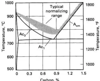
3.2.3. Normalizing
19 microstructure, areas that contain about 0.8% carbon are pearlitic. Those low in carbon are ferritic.
The somewhat higher austenitizing temperatures used for normalizing, as compared to those used for annealing hypoeutectoid steels, in effect produce greater uniformity in austenitic structure and composition similar to a homogenizing treatment, although at a much lower temperature and for shorter times than those used for homogenizing. Another of the major objectives of normalizing is to refine the grain size that frequently becomes very coarse during hot working at high temperatures or that is present in as-solidified steel castings. As such hot worked or cast products are heated through the Ac1
and Ac3 temperatures, new austenite grains are nucleated and, if the austenitizing
temperature is limited to the range in the Figure 3.5, a uniform fine-grained austenite is produced. Exceeding the indicated temperature range might result in excessive austenitic grain size. Normalizing, then, produces a uniform, fine-grained austenite grains structure that in hypoeutectoid steels transforms to ferrite-pearlite microstructures on air cooling. The resulting microstructure may have good uniformity and desirable mechanical properties for a given application or may be reaustenitized for final hardening by quenching to martensite (Krauss, 1980). Figure 3.6 gives a typical temperature profile during normalizing, also comparing to annealing.
20 Figure 3.6 – Comparison of time-temperature cycles for normalizing and full annealing.
The slower cooling of annealing results in higher temperature transformation to ferrite and pearlite and coarser microstructures than does normalizing (Kraus, 1980).
After hot worked, the steel is relatively coarse grain structure and perlite is widely dispersed. Then, during autenitization prior to quenching in a quench hardening treatment, homogeneous austenite may not be obtained during the normal (recommended) austenitizing cycle. Heating to higher temperatures and/or for longer times to obtain homogeneous austenite may lead to unacceptable large austenite grains size. Normalizing gives a general refinement of structure and facilitates the formation of homogeneous autenite during austenitizing, without much grain coarsening, as examplified in Figure 3.7.
21 3.2.4. Quenching
This chapter proposes to give only an introduction about quenching process. The main quenching aspects covering heat exchange between workpiece and quench bath are discussed later (Itens 3.5 and 3.6).
The material properties of steels are very important according to the component application. The outstanding importance of steels in engineering is associated with their ability to change its mechanical properties over a wide range when subjected to controlled heat treatment. Quenching is a common method of hardening steel. This process is based on a diffusionless process caused by a fast cooling rate. A quenching cycle is illustrated schematically in Figure 3.8 (a). It is possible to accelerate cooling from the solution-treating temperature and control the transformation of austenite to bainite and martensite to have higher strength and hardness than obtained with annealing and normalizing.
In order to demonstrate how cooling rate affects the phase transformations during quenching, Figure 3.8 compares the phase transformation for an AISI 4140 during fast (20°C/s) and slow (5°C/s) cooling rates. For a specific part, a significant amount of martensite is formed during cooling at 20°C/s, but much less at 5°C/s. Cooling at 5°C/s results in about 4% and 6% ferrite formed before the start of bainite (Bs) and martensite (Ms) formation, respectively.
22 The TTT diagram is defined for diffusion-controlled transformations. Bainite is one of the products obtained during quenching process. However, Voort (1991) observes that a horizontal line, labeled MS, appears on each TTT diagram. This line indicates the
temperature at which martensite (diffusionless transformation) starts to form on quenching from the austenitizing temperature. Upon further cooling below this temperature, more and more martensite will form. The percentage o austenite transformed to martensite as cooling progresses is commonly defined as a function of temperature. The temperatures may be indicated as MS, M50 and M90, representing the
temperatures in which the martensite begins to form, the austenite is half transformed and the austenite is 90% transformed, respectively.
According to Totten and Howes (1997), the most common quenchants in hardening practice are liquids including water, water that contains salt, aqueous polymer solutions, and hardening oils. Inert gases, molten salt, molten metal, and fluidized beds are also used. Quenching techniques used for liquid media are immersion quenching and spray quenching. Immersion quenching, where the part is submerged into an unagitated or agitated quenchant, is the most widely used. The part may be quenched directly from the austenitizing temperature to room temperature (direct quenching) or to a temperature above the MS temperature, where it is held for a specified period of time,
followed by cooling in a second medium at a slower cooling rate (time quenching or interrupted quenching). The quenching intensity can be changed by varying the type of quenchant, its concentration and temperature, and the rate of agitation. The heat transfer is mainly determined by the impingement density and its local distribution.
23
(a) (b)
Figure 3.9 – Typical (a) plate and (b) lath martensite (Krauss and Marder, 1971).
3.2.5. Hardenability
Martensite is the hardest microstructure that can be produced in any carbon steel. To obtain martensite through the transformation of austenite, mixtures of ferrite and cementite should be avoided. Thus, the maximum hardness that can be produced in any given steel is that associated with a fully martensitic microstructure. Therefore, the quenching process is used to obtain martensite, and also bainite, to increase the material hardness.
Qualitatively, Sharma (1996) defines hardenability as a property of steel which corresponds to its susceptibility to hardening upon quenching. The concept of hardenability is different of intensity of hardening. Hardness of quenched (martensitic) steels is essentially a function of their carbon content and generally refers to the hardness of 100% martensite structure. Hardenability, on the other hand, deals with the depth of hardening upon quenching finite sized samples. As an example, steel quenched to 100% martensite may have lower hardness but higher hardenability as compared to steel having higher hardness on quenching to 100% martensite.
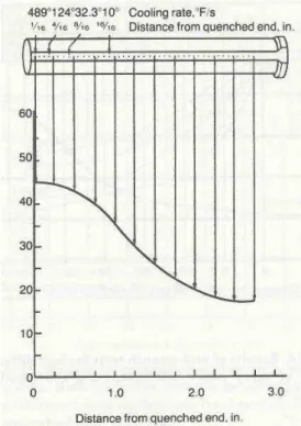
24 a series of round bars. The specimen is cooled at one end by a colum of water, thus the entire specimen experiences a range of cooling rates between those associated with water and air cooling. After quenching, parallel flats ground on opposite sides of the specimen, and hardness readings are taken along the bar starting from the quenched end, and plotted as shown in Figure 3.10 (Krauss 1980).
Figure 3.10 – Method of plotting hardness data from an end-quenched Jominy specimen (Melloy, 1977; in Krauss, 1980).
25 Figure 3.11 - Microstructure change along the Jominy quench bar for (a) 4140, and (b)
5140 alloys (Guo et al., 2009).
The material hardness is cooling rate dependent. The hardenability is different for each steel composition. For AISI 4140 steel, Figure 3.12 relates cooling rate and hardenability superposed on TTT and CCT diagrams. It can be observed that martensite and bainite are the hardest phases compared to ferrite and perlite.
26 The effectiveness of a given quenching medium is ranked by a parameter referred to as its “severity of quench”. This measure of cooling or quenching power is determined experimentally by quenching a series of round bars of given steel (Krauss, 1980). Figure 3.13 shows schematically the results of oil and water quenching bars of SAE 3140 steel. The cross-hatched areas represent the unhardened areas of the various bars, assuming that less than 50% martensite represents an unhardened microstructure. The larger the bar diameter, the greater the unhardened diameter. Oil-quenched bars also produce larger nothardened diameters when compared to water-quenched bars.
Figure 3.13 – Schematic representation of extend of hardening in oil-quenched and water-quenched bars of SAE 3140 steel of various diameters. The cross-hatched areas
represent the unhardened core (Grossmann and Bain, 1964).
3.3. Stress
3.3.1. Principal Stress
Hosford and Caddell (2007) define the stress as the intensity of force, F, in a specific point:
(3.1)
where A is the area that undergoes F.
When the stress is constant over a given area, the following relation can be written:
27 Figure 3.14 (a) shows a bidimensional perspective of the beginning of a compressive process. The cylindrical workpiece is divided in small elements, and the stresses in each one can be analyzed as shown in Figure 3.14 (a) and (b). The stress is divided in 9 components. The normal component is referred to the one in which the force is applied on the normal direction to the plane. The normal stress may be tensile or compressive. The shear components are the stresses parallel to the plane.
Figure 3.14 – Stress acting on an element. (a) Cylinder upsetting process. (b) Forces acting on an element. (c) Stress components acting on an element (Altan et al., 2005).
Stress components are defined with two subscripts. The first indicates the normal direction to the plane, and the second indicates the force direction. The normal stresses are compressive when negative, and tensile when positive. This collection of stresses is referred to as the stress tensor:
. (3.3)
The stresses expressed along one set of axes may be expressed along any other set of axes. In Figure 3.15 the force on direction can be calculated as , and the area normal to will be . So,
. (3.4)
28
. (3.5)
Figure 3.15 – The stresses acting on a plane, , under a normal stress, (Hosford and Caddell, 2007).
It is possible to define a set of axes in which the shear stresses become zero. In this case, the normal stresses , e will be called principal stresses. The principal stress magnitudes, , are calculated:
(3.6)
where , e are called the invariants of the stress tensor:
,
e (3.7)
.
The first invariant where is the pressure. , e are not dependent on the orientation of the axes. Expressing them as a function of principal stresses, they are:
,
e (3.8)
.
3.3.2. Effective Stress
29 the yielding starts when the yield strength, , is reached. For each situation with a particular stress combination, the yielding is related for a particular combination of principal stresses.
The effective stress, , is a very practical and useful definition. It is given by a function of the principal stresses, and can also be related, for example, to a yielding criterion. A yielding criterion is a postulated state of stress that will cause yielding, indicating that it will occur in case the effective stress reaches a critical value.
During plastic deformation, the effective stress concept is still valid, and is used as a useful parameter in order to define the behavior in a specific point of a system. Two main criterias are used: Tresca and von Mises ones. Since this work is based on a CAE tool, which approaches effective stress based on von Mises criterion, the here described theory is based von Mises criterion. Tresca criterion is simpler than von Mises criterion, and does not consider the intermediary stress. However, Tresca criterion is more used for engineering projects, while von Mises is used for theoric works, since it is more precise.
Von Mises criterion postulates that yielding will occur when the following mathematical expression reaches a critical value:
, (3.9)
or
. (3.10)
The critical value may be found considering a uniaxial tensile test in the 1-direction. Substituting e during yielding, the de von Mises criterion can be written as:
. (3.11)
A general equation can be expressed as follows:
30 Figure 3.16 represents a graph with possible combination for yielding, assuming that
. The tridimensional Tresca and von Mises criterions can be visualized in Figure 3.17. The Tresca criterion is a regular hexagonal prism and the von Mises criterion is a cylinder. Both criterions are centered on a line .
Figure 3.16 - Tresca and von Mises loci showing certain loading paths (Hosford and Caddell, 2007).
Figure 3.17 - Three-dimensional plots of the Tresca and von Mises yield criterion (Hosford and Caddell, 2007).
Finally, according to Von Mises criterion, the effective stress is:
31 3.3.3. Residual Stress
Residual stresses are present in parts after any process that strains the material heterogeneously. A number of thermal and mechanical processes produce residual stresses that might be detrimental to the performance of fabricated steel parts or assemblies. Heavy metalworking such as forging, rolling, and extrusion causes stresses that remain in the metal if the work is performed below the hot-working temperature. Heat treatment processes are also sources of residual stresses.
Residual stresses can be defined as resulting stresses in equilibrium in components that are not undergoing external stresses. They are the result of nonhomogeneous elastic e/or plastic deformation, due to plastic work or phase transformations with volume changing, affecting the state of strain along the workpiece. As an example, Dieter (1988) considers a metal specimen where the surface has been deformed in tension by bending so that part of it has undergone plastic deformation. When the external force is removed, the regions which have been plastically deformed prevent the adjacent elastic regions from undergoing completely elastic recovery to the unstrained condition. Thus, the elastic deformed regions are left in residual tension, and the regions which were plastically deformed must be in a state of residual compression to balance the stresses over the cross section of the specimen. Figure 3.18 gives possible situations in which applied and residual stresses are superposed.
32 Figure 3.18 – Superposition of applied and residual stresses. (a) Elastic stress distribution with no residual stress; (b) residual stress distribution produced by shot
peening; and (c) the algebraic summation of external bending stresses and residual stresses (Dieter, 1988).
33 Figure 3.19 - Schematic illustration showing the development of residual stresses on
cool-down of a metallic material which undergoes no allotropic transformation on cooling. Only longitudinal stresses are shown (Ebert, 1978).
34 by which they originate. The main groups of residual stresses are: casting, forming, working-out, heat treatment, joining and coating residual stresses.
Figure 3.20 – Schematic of all three kinds of residual stresses in a two-phase material after quenching and their superposition (Liscic et al., 1992).
Compressive residual stresses are desirable in a finished component to enable it to resist applied stress systems. However some stresses originated during manufacturing will be relieved during heating as the stress system readjusts. Residual stresses due to heat treatment processes may distort and crack components, making them not satisfactory for service. In addition, residual stresses from heat treatment may distort parts during subsequent manufacturing such as machining. The residual stresses may also result in failure in service below design stresses. The maximum value of the residual stress which can be produced is equal to the elastic limit of the material.
35 (2006) used numerical techniques to predict residual stresses after quenching of a forged aluminum block, and the predictions were compared with experimental measurements. Looking for reducing residual stresses, they performed two different methods of cold working (compression and stretching) which are commonly used to reduce the residual stresses. The comparison of results showed that both compression and stretching processes reduced the residual stresses more than 90% (Figure 3.21).
Figure 3.21 – x-, y- and z-component residual stress of an aluminum block along x-locus after quenching, compression, and stretching (Koç et al., 2006).
3.4. Strain
3.4.1. Definition
36 deformed. The line has been translated, rotated, and deformed. The deformation is characterized by the engineering or nominal strain, e:
3.14
However, an alternative definition is called true or logarithmic strain, which is a nonlinear strain measure that is dependent upon the final length of the model:
3.15
Figure 3.22 - Deformation, translation, and rotation of a line in a material (Hosford and Caddell, 2007).
Strains may be caused by mechanical work, heat and heat treatment processes, including all boundary conditions of each specific system. For deformation, the total incremental strain is assumed to consist of several components:
3.16 where , , , , and represent the entities for elastic, plastic, thermal, phase transformation and transformation plasticity, respectively. The phase transformation occurs from phase to phase .
3.4.2. Elastic, Plastic and Thermal Strain
37 For elastic behavior, Hooke’s laws can be expressed as:
,
, 3.17
,
and,
,
, 3.18
,
where is Young’s modulus, is Poisson’s ratio, is shear strain, is shear stress, and is the shear modulus. For an isotropic material, , , and are interrelated by:
, or 3.19
. 3.20
In manufacturing processes such as metal forming, permanent deformations are desired. Plastic strain is the term used for permanent strain. According to yielding criterion (i.e. von Mises), a postulated state of stress will cause yielding, and therefore plastic strain, indicating that yielding will occur in case the effective stress reaches a critical value. The incremental plastic work per volume is the effective strain, , defined below:
3.21
The von Mises strain may be expressed as:
3.22
For proportional straining with a constant ratio of , the total effective strain is:
3.23
38 heat and cooling processes change the workpiece temperature. This temperature changing expands or shrinks the part. Therefore, thermal strain occurs when coefficient of thermal expansion is specified and a temperature change is applied:
, 3.24
where is the thermal expansion coefficient, and is the reference temperature.
Depending on the system boundary conditions, the material dilatation can elastically and plastically deform the material. In addition, plastic flow, especially at elevated temperature, can be considered a thermally activated process (Dieter, 1988).
3.4.3. Phase Transformation and Transformation Plasticity Strain
39 Figure 3.23 – Body-centered tetragonal crystal structure of martensite in Fe-C alloys. Carbon atoms are trapped in one set (z) of interstitial octahedral sites. The x and y sites
are unoccupied (Cohen, 1962; in Krauss, 1980).
Figure 3.24 – Thermal expansion and contraction curves for 4340 steel (Bates et al., 1991).
Phase transformation strain is a consequence of the structure change during the transformation. As a result of phase transformation, the material may change its volume. The volume change due to transformation is induced by a change in the lattice structure of the metal. This amount of strain is in the form of:
, 3.25
where is the fractional length change due to transformation, is the transformation volume fraction rate, and is the Kronecker delta.
40 the dimensional changes due to transformation induced volume change. For FE simulation, the equation for transformation plasticity can be considered as:
, 3.26
where is the transformation plasticity coefficient, , is the volume fraction rate, and is the deviatoric stress tensor. A general range for for steel is (SFTC, 2010):
austenite phase to ferrite, pearlite or bainite phase: between 4 and 13 (x10-5/MPa);
austenite to martensite: between 5 and 21 (x10-5/MPa);
and ferrite or pearlite to austenite: between 6 and 21 (x10-5/MPa).
3.5. Stress-Strain Curves
3.5.1. The Tension Test
Tension tests are used to measure the effect of strain on strength. Sometimes other tests, such as torsion, compression, and bulge testing are used, but the tension test is simpler and most commonly used. Moosbrugger (2002) explains that the simplest loading to visualize is an one-dimensional tensile test, in which a uniform slender test specimen is streched along its long central axis. The stress-strain curve is a representation of the performance of the specimen as the applied load is increased monotonically usually to fracture. Stress-strain curves are usually represented as:
“Engineering” stress-strain curves, in which the original dimensions of the specimen are used in most calculations;
“True” stress-strain curves, where the instantaneous dimensions of the specimen at each point during the test are used in the calculations. This results in the true curves being above the engineering curves, notably in the higher strain portion of the curves.
41 plastic, or nonrecoverable. In a ductile material, the force reaches a maximum and then decreases until fracture. Figure 3.25 shows a typical engineering stress-strain curve obtained through a FE simulation. The engineering stress-strain curve is compared to the true stress-strain curve, obtained from the effective stresses and strains up to necking start, in Figure 3.26 for the plastic behavior.
(a) (b)
Figure 3.25 – Simulated tension test: (a) axisymmetric specimen (dimensions in mm) and (b) tension test for cooper (da Silva et al., 2010).
Figure 3.26 – Simulated tension test for cooper (da Silva et al., 2010).
42
, 3.27
and the engineering strain, , is calculated as
, 3.28
where, is the original gauge length, and is the elongation of during the test.
Several basic mechanical material properties are shown in Figure 3.27, and described by Server et al. (2011) as follows:
Yield Strength ( ): indicates the start of plastic deformation. is determined approximately by drawing a parallel line to the linear elastic region of engineering stress-strain curve from 0.2% engineering strain. The intersection of this parallel line with the engineering stress-strain curve gives the value of . Ultimate Tensile Strength (UTS) is the maximum engineering stress in a tensile
test and is connected to the end of uniform elongation and start of localized necking.
Elastic Modulus ( ) (also known as Young’s Modulus) is the slope of the elastic part of an engineering stress-strain curve.
e0 is the elongation at yield strength ( ).
Uniform elongation ( ) is the elongation at the maximum load.
Total elongation ( ) (also known as elongation at break) is the total elongation of the original gage length of a tensile specimen at fracture. This includes both uniform ( ) and post-uniform elongations.
Area Reduction ( ) is the percentage of reduction in the area, and calculated by cross section area at fracture ( ) and initial cross section area (A0):
43 Figure 3.27 – A tensile-test sequence showing different stages in the elongation of the
specimen (Kalpakjian and Schimd, 2006).
The true stress is based upon the instantaneous cross sectional area, ,
, 3.30
where, . Before necking, the true strain can be calculated as:
. 3.31
After necking, the true strain must be based on the area:
. 3.32
3.5.2. Determining the True Stress-Strain Curve with Yield and Ultimate Tensile Strengths
In some situations, a few material properties are known. For some applications, such as simulation proposes, it is necessary to obtain the behavior of the material based on the true stress-true strain curve, shown in Figure 3.26 for the plastic region (flow stress curve). Elastic region is linear and can be defined according to the Hooke’s Law:
44 The flow stress curve can be approximated by the power-law expression, also called the Hollomon equation,
, 3.34
where, is the strength coefficient and is the strain hardening exponent.
Hosford and Caddell (2007) demonstrated that at UTS, . Since , when
, . So, , and the maximum load
corresponds to . Considering the power law and solving this equation, the true stress at the maximum load can be expressed as
. 3.35
As it can be analyzed in Figure 3.27, points P1 and P2 represent Y and UTS, respectively. Since Y and UTS are known, a system of two equations, power law, is solved. Equation 3.34 is applied for Y, and Equation 3.35 is applied for UTS. The strain at P1 changes depending on material and it is larger than 0.2% engineering strain. For steel, it may be assumed it is 0.6% (Server et al., 2011). In case the Young’s Modulus, E, is known, the strain at P1 can be defined, and the curve more precise. For this method, it is assumed that the effect of the strain rate is neglected and the strain hardening exponent, n, does not change with strain.
3.6. Interface Conditions between Workpiece and Environment
3.6.1. Heat Transfer during Air Cooling
Processes such as normalizing are usually used to eliminate some microstructural irregularities and to refine the grain structure of hot worked steels, and for general refinement of structure prior to quenching hardening treatment. The austenitized part during normaling process is air cooled. The mechaninsm of heat transfer between steel components and enviroment are convection and radiation.
45 transferred by the bulk, or microscopic, motion of the fluid. It is costumary to use the term convection when referring to this cumulative transport and the term advection when referring to transport due to bulk fluid motion. Convection heat transfer may be classified as forced or free (natural) convection (Figure 3.28). Boiling and Condensation are also heat transfer processes. Regardless of the particular nature of the convection heat transfer process, the appropriate rate equation is of the form:
, 3.36
where is the convective heat flux, is the convection heat transfer coefficient, and and are surface and fluid temperature, respectively.
Figure 3.28 – Convection heat transfer processes; (a) forced convection and (b) natural convection (Incropera et al., 2007).
Thermal radiation is energy emitted by matter that is at a nonzero temperature. The energy of the radiation field is transported by electromagnetic waves. There is an upper limit for the emissive power, which is described by the Stefan-Boltzmann law:
, 3.37
where is the Stefan-Boltzmann constant ( ). The heat flux emitted by a real surface is given by:
, 3.38
46 Bamberger and Prinz (1986) have investigated the heat transfer coefficients for various cooling methods. For air cooling, Figure 3.29 shows the coefficients of heat transfer by means of convection and radiation.
Figure 3.29 – Heat transfer coefficients for air cooling as function of surface temperature (Bamberger and Prinz, 1986).
3.6.2. Radiation Exchange between Surfaces
During heating and cooling processes, components being heat treated may be disposed close to other components. In this case, the temperature profile of each part may change due to the proximity of other parts in the same process. Since a body radiates energy to environment, other bodies may be part of the environment, and part of the system as a consequence.