FINITE ELEMENT MODELLING OF THERMO-ELASTOPLASTIC BEHAVIOUR OF HOT-ROLLED STEEL PROFILES SUBMITTED TO FIRE

FINITE ELEMENT MODELLING OF THERMO-ELASTOPLASTIC

BEHAVIOUR OF HOT-ROLLED STEEL PROFILES

SUBMITTED TO FIRE

Fonseca, Elza M. M.*y Vila Real, Paulo M. M.† *

Departamento de Mecânica Aplicada Instituto Politécnico de Bragança Campus de Sta. Apolónia, apartado 134

5300 Bragança, Portugal

e-mail: efonseca@ipb.pt, Tel.: 351 73 3303094, Fax: 351 73 313051

†

Departamento de Engenharia Civil Universidade de Aveiro

Campus de Santiago 3810 Aveiro, Portugal

e-mail: pvreal@civil.ua.pt, Tel.: 351 34 370049, Fax: 351 34 370953

Key words: Fire, Thermo-elastoplasticity, Eurocodes, Heat Conduction, Non-Linearity, Standard temperature-time curve ISO 834, Finite Elements

1 INTRODUCTION

A finite element program FEMSEF98 – “Finite Element Modelling of Structures Exposed to Fire” has been developed to model the thermo-elastoplastic behaviour of hot-rolled steel profiles exposed to fire. Heat conduction is assumed for the heat transfer analysis and an elastoplastic model is employed to predict the development of thermal stresses and strains. In this paper the elastoplastic analysis is done using the Prandtl-Reuss’s theory1,8 for incremental plastic analysis.

A finite element formulation of the heat conduction in solids is presented, giving particular attention to the non-linearity of the problem. This non-linearity is treated by an iterative procedure based on the modified Newton-Raphson method, where in the original jacobian matrix the unysymmetric term is neglected3.

The simplified heat conduction equation of the eurocode 3 is also non-linear wherefore an iterative procedure is also needed.

2 FORMULATION OF THERMO-ELASTOPLASTIC BEHAVIOUR

Neglecting the heat generated during the deformation, the thermal and the mechanical problems are uncoupled. So the technique involves concurrently solving an uncoupled set of equations, the transient heat conduction equation and the incremental equilibrium equation, within each time interval. The same finite element formulation (finite element mesh, shape function, etc.) and the same equation solution technique (frontal solution technique) are used in both the thermal and stress analysis.

2.1 Thermal analysis: the heat conduction equation and its boundary conditions

The governing equation for transient heat conduction in the domain Ω takes the form

t c

Q _p

∂ ∂θ ρ = + θ ∇ λ

∇_{( )} & ₍₁₎

where λ is the thermal conductivity, Q& the heat generated/unit volume, ρ the density, c_p the specific heat, θ the temperature and t the time. The temperature field which satisfies eq. (1) in

Ω, must satisfy the following boundary conditions: prescribed temperatures θ on a part Γ_θ of the boundary; specified heat flux q on a part Γ_q of the boundary; heat flux by convection between a part Γ_c of the boundary at temperature θ, and the environment at the temperature

∞

θ

) (θ−θ_∞

= _c

c h

q on Γ_c (2)

where h_c is the heat transfer coefficient by convection; heat flux by radiation between a part

) ( ) ( ) )( ( )

( 4 4 2 2

r a r a

h a a a h q r θ − θ = θ − θ θ + θ θ + θ βε = θ − θ βε = 4 4 4 3 4 4 4 2

1 on Γr (3)

where β is the Stefan-Boltzmann constant, ε is the emissivity and h_r is the heat transfer coefficient by radiation. If the heat flux is simultaneously by convection and radiation and if in particular θ_∞ =θ_a, we can write

) ( ) ( )

(θ−θ_∞ + θ−θ = θ−θ_∞

= +

= _{c r c r a cr}

cr q q h h h

q (4)

where h_cr =h_c+h_r is the combined convection and radiation heat transfer coefficient.

2.1.1 Finite element discretization and time integration

Using finite elements Ωe to discretize the domain Ω, a weak formulation and the Galerkin method for choosing the weighting functions, we obtain2 the following system of differential equations

F

θ

C

θ

K + & = (5)

where

(

)

_∑∫

∑∫

e N N d h N N d

K 1 1 (6)

∑∫

lm e c N N d

C 1 (7)

∑∫

∑∫

∑∫

= Γ ∞

= Γ = Ω Γ θ + Γ − Ω = H e e h cr l Q e e q l E e e l

l N Qd N qd N h d

F _e h e q e 1 1 1

& ₍₈₎

where E is the total number of elements, Q is the number of elements with boundary type Γ_q, H is the number of elements with boundary type Γ_c and/or Γ_r, N_l and N_m are shape functions.

Using a finite difference technique to discretize the time, the system of ordinary differential equations (5) results in the recurrence formula:

α + α + α

+ n = n

n θ F

Kˆ ˆ 0< ≤α 1 (9)

where $

K_n K_n C_n

t

+α = +α+_α +α

1

∆ (10)

n n n

n

tC θ F

F_{+α +α +α}

∆ α +

= 1

Having solved the system of equations (9) for θ_n+α, at time t_n+α, the value of θ at the end of the time interval ∆t, that is, at time t_n+1 is given by

n n

n θ θ

θ 

    

α − + α

= _+α

+

1 1 1

1 (12)

Varying the value of the parameter α, we can obtain several time integration schemes2, like the Crank-Nicolson scheme for α=1 2, the Galerkin scheme for α=2 3 and the Euler Backward scheme forα=1.

2.1.2 Iterative procedure for the solution of the non-linear thermal transient problem

In non-linear problems, where the thermal properties of the material are temperature dependent, the system of equations (5) can generally be written as

) , ( ) ( ) , ( ) ( ) ,

(θ t θ t Cθ t θ t F θ t

K + & = (13)

There is not a general method to solve this system of non-linear differential equations. However, several numerical solution procedures, in essence, based on a linear time integration and an iterative process are available2,3,4,5,6. Here, an effective algorithm for the analysis of non-linear transient thermal problem is presented. The matrices K and C and the vector F, needed to construct Kˆ _n+α and Fˆ_n+α, given by eq. (10) and (11), can vary throughout the time interval ∆t as functions of the unknown vector temperature θ and time t. Therefore, these matrices must be evaluated at time t_n+α and the temperature θ_n+α, so that

) , ( _{+α +α} α

+ = n n

n K θ t

K (14)

) , ( _{+α +α} α

+ = n n

n K θ t

K (15)

) , ( _{+α +α} α

+ = n n

n K θ t

K (16)

In order to fully satisfy these non-linear conditions of the problem, it is necessary to employ an iterative procedure in each time step. In this algorithm a modified Newton-Raphson method is adopted3,4 ,5. During any step, i, of the iterative process of solution, eq. (9) will not generally be satisfied unless convergence has occurred. Therefore a system of residual forcesψ will exist, so that

0 ˆ

ˆ ₋ 1 _≠

= +

α + α + α + α

+ in

i n i

n i

n F K θ

ψ (17)

The improved value of θi_n+₊1_α can be obtained by

[ ]

n i

n i

n +α

− α + α

+ =

∆θ Kˆ 1ψ (18)

i n i

n i

n +α +α

+ α

+ =θ +∆θ

θ 1

(19) The iterative procedure is then continued, solving a set of linearized equations (18) for

i n+α

∆θ at every iteration step, until the solution converges to the non-linear solution.

The quasi-stiffness matrix Kˆi_n+α in (18) is a linearized tangential stiffness matrix which corresponds to the Jacobian matrix of the standard Newton-Raphson method, but in which the unsymmetrical term is neglected3.

The convergence criteria employed is as follows:

TOL

i n i n

< ∆

+ α +

α +

1

θ θ

(20)

where

TOL is the specified tolerance.

⋅ denotes the Euclidean vector norm. i

n+α

∆θ is the temperature change in the ith iteration.

1

+ α + i n

θ is the current temperature value.

2.2 Mechanical analysis

In the mechanical model, the onset of plastic behaviour is governed by a yield criteria dependent of stress level and from the plastic deformation by a general formula:

) , ( ) ( ) , ,

(σ K θ = f σ −Y K θ

F _{ij ij}

(21)

where, f(σ_ij) is a yield function; Y(K,θ), is a function that depends on a material hardening parameter, K, and the temperature, θ.

When the plastic flow occurs, the loading function will vary according to the equation:

0

= θ θ ∂ ∂ + ∂

∂ + σ σ ∂

∂

= dK F d

K F d

F

dF _ij

ij

(22)

The flow rule governs the plastic flow after yielding and it will be assumed that the plastic strain incremental is proportional to the stress gradient of a plastic potential, so that:

ij p

ij

Q d d

σ ∂

∂ λ =

ε (23)

where Q is a plastic potential function and dλ is the proportionality constant termed the plastic multiplier.

ij p

ij

f d d

σ ∂

∂ λ =

ε (24)

since it has been postulated that both are functions of J2’ and J3’.

2.2.1 The thermo-elastoplastic strain increment

The model is based upon the Prandtl-Reuss incremental plasticity theory11. Assuming small strains, the complete incremental relationship between stress and strain for thermo-elastoplastic deformation is found to be

th ij p ij e ij t

ij d d d

dε = ε + ε + ε (25)

The elastic strain increment is given by Hooke law:

kk ij ij

e

ij d

E d

d + − ν δ σ

µ σ =

ε (1 2 )

2

'

(26)

The plastic strain increment is done by equation (24) and finally the thermal strain is done by

ij th

ij d

dε =α(θ) θδ (27)

where: α(θ) is the thermal expansion coefficient, which can be temperature dependent. The Von Mises yield criterion is formulated by the second deviatoric stress invariant, J2’ ,

written as

) , ( )

( 3 ' 12

2 =σ K θ

J _y (28)

The incremental stresses occurring in the time interval are done:

th j

ij ij th ij ep ij

ij D d d D d d a d

dσ = ε + σ = ( ε − λ )+ σ (29)

where Dijep is the elastoplastique matrix.

The application of the virtual work principle gives finally the system of algebraic equations to be solved. This is done in the code FEMSEF98 using a modified Newton-Raphson method.

3 STEEL PROPERTIES ACCORDING TO THE EUROCODE 3

The thermal and mechanical properties of steel as function of the temperature shall be determined from the following.

3.1 Mechanical properties of steel

3.1.1 Strength and deformation properties

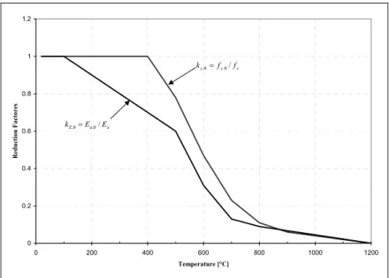
stress-strain relationship for steel at elevated temperatures, as follows:

- effective yield strength, relative to yield strength at 20ºC: k_y,θ = f_y,θ/ f_y - slope of linear elastic range, relative to slope at 20ºC: k_E,θ =E_a,θ/E_a

At 20 ºC the Eurocode 1 gives the following values: f_y =235×103kN/m2 and

2 6

/ 10

210 kN m

E_a = × .

0 0.2 0.4 0.6 0.8 1 1.2

0 200 400 600 800 1000 1200

Temperature [°C]

Reduction Factores

y y

y f f

k,θ= ,θ/

a a

E E E

k,θ= ,θ/

Fig. 1 – Dependency with temperature of the reduction factors k_y,θ,com and k_E,θ,com

3.1.2 Unit mass

The unit mass of steel ρ_a may be considered to be independent of the temperature. The following value has been taken

3

/ 7850kg m

a =

ρ (30)

3.2 Thermal properties 3.2.1 Thermal elongation

Assuming a simple calculation model the relationship between thermal elongation and steel temperature may be considered to be constant, being the elongation determined from:

) 20 (

10 14

/ = × 6 θ −

∆ −

a

l

3.2.2 Specific heat

The specific heat of steel c_a [JkgK], figure 2, may be determined from the following:

         ≤ θ ≤ < θ ≤ − θ + < θ ≤ θ − + < θ ≤ θ × + θ × − θ × + = − − − C C C C C C C C C a a a a a a a a a a º 1200 º 900 650 º 900 º 735 731 17820 545 º 7350 º 600 738 13002 666 º 600 º 20 10 22 . 2 10 69 . 1 10 73 . 7

425 1 3 2 6 3

(32)

0 5 0 0 1 0 0 0 1 5 0 0 2 0 0 0 2 5 0 0 3 0 0 0 3 5 0 0 4 0 0 0 4 5 0 0 5 0 0 0

0 2 0 0 4 0 0 6 0 0 8 0 0 1 0 0 0 1 2 0 0 (º C)

Fig. 2 – Dependency with temperature of the specific heat, [J/KgK]

3.2.3 Thermal conductivity

0 10 20 30 40 50 60

0 200 400 600 800 1000 1200

(ºC)

Fig. 3 – Dependency with temperature of the thermal conductivity, [W/mK]

4 STEEL TEMPERATURE DEVELOPMENT FOR UNPROTECTED INTERNAL STEELWORK

For an equivalent uniform temperature distribution in the cross-section, the increase of temperature ∆θ_a,t in an unprotected steel member during a time interval ∆t may be determined from 10:

t h c

V A

d net a a m t

a = _ρ ∆

θ

∆ _, / & _{, (34)}

where: V

A_m/ - is the section factor for unprotected steel members, [m-1]; m

A - is the exposed surface area of the member per unit length, [m2/m]; V – is the volume of the member per unit length, [m3/m];

a

c - is the specific heat of steel from (32) ,[J/kgK];

a

ρ - is the unit mass of steel, from (30), [kg/m ]; 3

d net

h& _, - is the design value of the net heat flux due to convection and radiation per unit area9:

r net r n c net c n d

net h h

h& _, =γ _, & _, +γ _, & _, [W/m2]; c

n,

γ - factor to account for different national types of test and equals [1.0]

r n,

γ - is equal to [1.0] as γ_n,c; ) (

,c c g m net

h& =α θ −θ [W/m2];

c

α - is the coefficient of heat transfer by convection, which must be taken9 as 25 W/m2K;

g

In this work it was adopted the standard temperature-time curve ISO 834, which is given by:

) 1 8 ( log 345

20+ ₁₀ +

=

θ_g t [ºC];

t – time in minutes [min];

m

θ - surface temperature of the member;

] ) 273 (

) 273 [(

10 67 ,

5 8 4 4

, =Φ⋅ε ⋅ × ⋅ θ + − θ +

−

m r

res r

net

h& [W/m2];

Φ - is the configuration factor, which should be taken9equals [1.0]; f

m res =ε ⋅ε

ε - is the resultant emissivity; 625

, 0

=

ε_m - is the emissivity related to the surface material10; 8

, 0

=

ε_f - is the emissivity related to the fire compartment 9,10; r

θ - is the radiation temperature of the environment of the member usually taken as θ_r =θ_g;

t

∆ - time interval, which should not be taken as more than 5 seconds10.

5 THERMOMECHANICAL BEHAVIOUR OF STEEL COLUMNS EXPOSED TO THE STANDARD FIRE CURVE ISO 834

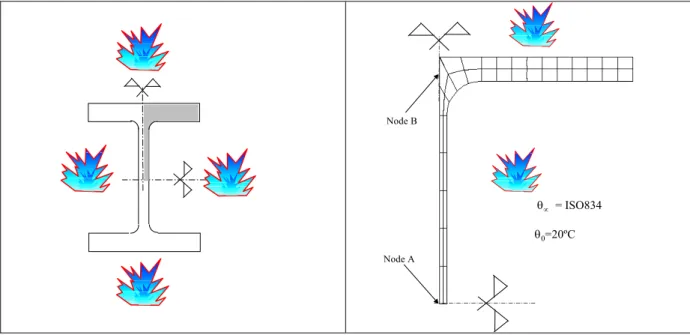
Results of the numerical modelling of the thermomechanical behaviour of hot-rolled profiles of the IPE, HEA, HEB and HEM series exposed to the standard fire curve ISO 834, acting on the four sides of the profile, as it can be seen in figure 4.a, are shown.

Due to the symmetry, only a quarter of the profile was analysed, being the finite element mesh used represented in figure 4.b.

Node A Node B

θ0=20ºC θ∝ = ISO834

In figure 5 we can see the variation of the section factor for all the profile series analysed in this paper.

Am / V = P / A

Node A Node B

0 50 100 150 200 250 300 350 400 450

S

e

ct

ion Fa

ct

o

res

IPE

HEA HEB HEM

80 / 100 Profiles Series 600 / 1000

Fig. 5 – Section factors.

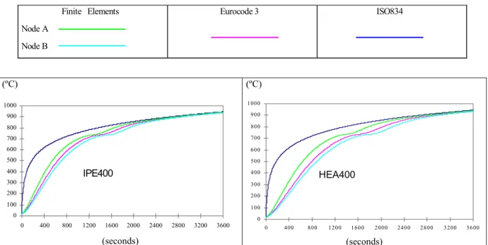
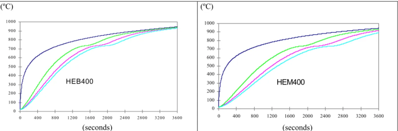
In figure 6 we can see the time history of temperature at node A and B for all profiles of the 400 series, using the simplified equation of the Eurocode 3 and the finite element results of FEMSEF98. It can be seen that the values of the temperature obtained from the Eurocode 3 equation are always between the values of the temperature of nodes A and B obtained using a finite element analysis. This shows that the values of the temperature of EC3 can be considered as an average value of the highest and lowest temperature in the profile.

Finite Elements

Node A

Node B

Eurocode 3 ISO834

(ºC)

0 100 200 300 400 500 600 700 800 900 1000

0 400 800 1200 1600 2000 2400 2800 3200 3600

( )

IPE400

(seconds)

(ºC)

0 10 0 20 0 30 0 40 0 50 0 60 0 70 0 80 0 90 0 1 00 0

0 40 0 80 0 1 2 00 16 0 0 2 0 00 24 0 0 2 80 0 3 20 0 3 6 00 HEA400

(seconds)

(ºC)

0 100 200 300 400 500 600 700 800 900 1 000

0 40 0 800 1 200 16 00 20 00 24 00 280 0 320 0 3600

HEB400

(seconds)

(ºC)

0 100 200 300 400 500 600 700 800 900 1000

0 400 800 1200 1600 2000 2400 2800 3200 3600

HEM400

(seconds)

Fig. 6 – Time history of temperature of nodes A and node B (fig. 4) for all profiles series 400, obtained using the FEMSEF98 and the simplified Eurocode 3 equation.

Figure 7 shows the temperature evolution of node A for all the profile series, obtained using the finite element solver FEMSEF98. As the section factor decreases the temperature field, decreases too, with an exception of the profile series HEM.

(ºC)

0 1 0 0 2 0 0 3 0 0 4 0 0 5 0 0 6 0 0 7 0 0 8 0 0 9 0 0 1 0 0 0

0 4 0 0 8 0 0 1 2 0 0 1 6 0 0 2 0 0 0 2 4 0 0 2 8 0 0 3 2 0 0 3 6 0 0 IPE80

IPE600

a) (seconds)

(ºC)

0 1 0 0 2 0 0 3 0 0 4 0 0 5 0 0 6 0 0 7 0 0 8 0 0 9 0 0 1 0 0 0

0 4 0 0 8 0 0 1 2 0 0 1 6 0 0 2 0 0 0 2 4 0 0 2 8 0 0 3 2 0 0 3 6 0 0 HEA100

HEA1000

b) (seconds) (ºC)

0 1 0 0 2 0 0 3 0 0 4 0 0 5 0 0 6 0 0 7 0 0 8 0 0 9 0 0 1 0 0 0

0 4 0 0 8 0 0 1 2 0 0 1 6 0 0 2 0 0 0 2 4 0 0 2 8 0 0 3 2 0 0 3 6 0 0 HEB100

HEB1000

c) (seconds)

(ºC)

0 1 0 0 2 0 0 3 0 0 4 0 0 5 0 0 6 0 0 7 0 0 8 0 0 9 0 0 1 0 0 0

0 4 0 0 8 0 0 1 2 0 0 1 6 0 0 2 0 0 0 2 4 0 0 2 8 0 0 3 2 0 0 3 6 0 0 HEM100

HEM300 HEM300 HEM1000

d) (seconds)

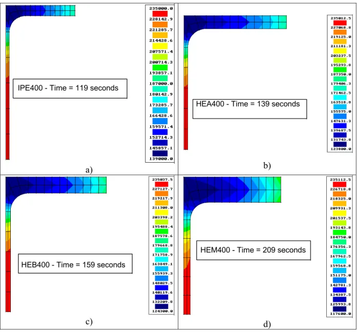
Figure 8 shows the stress field for the time instant correspondent to the onset of the plastic behaviour in the size 400 of all the profile series, obtained by FEMSEF98 considering plane strain conditions. The numerical values in the boxes represent the time correspondent to the beginning of plastic behaviour in each 400 profile series.

IPE400 - Time = 119 seconds

a)

HEA400 - Time = 139 seconds

b)

HEB400 - Time = 159 seconds

c)

HEM400 - Time = 209 seconds

d)

Fig. 8 – Equivalent stresses fields. a) IPE400; b) HEA400; c) HEB400; d) HEM400

Table 1

Profile Section Factor

[1/m]

Onset of plasticity

[s]

σeq min Time

[s]

σeq min Time

[s]

σeq min

IPE400 174 119 139 120 143.2 126 152.8

HEA400 120 139 123.8 140 127.1 148 137.3

HEB400 97 159 124.3 160 127.3 164 131.1

HEM400 62 209 117.6 210 119.9 214 122.5

The same results are shown in table 2 for other profile series.

Table 2

Profile Section Factor

[1/m]

Onset of plasticity

[s]

σeq min

IPE80 429 77 183.2 IPE400 174 119 139 IPE600 129 147 138.1

HEA100 264 97 152

HEA400 120 139 123.8

HEA600 89 178 115.4

HEB100 218 110 184.5

HEB400 97 159 124.3

HEB1000 78 195 115.4

HEM100 116 171 197

HEM400 62 209 117.6

HEM1000 70 208 115.1

6 CONCLUSIONS

A computational program based on the finite element method to model the thermo-elastoplastic behaviour of steel structural members exposed to the standard fire curve ISO 834 has been developed. This program has been used to study the thermo-mechanical behaviour of hot-rolled steel profile submitted to fire.

The results obtained with the developed program have been compared with the results obtained with the simplified heat conduction equation of the Eurocode 3. From this comparison we can conclude that the values of the temperature obtained from the Eurocode 3 equation are always between the values of the highest and lowest temperature obtained with the finite element analysis. The Eurocode results can be considered as an average of these two values.

ACKNOWLEDGEMENTS

This work was done within the framework of the project nº PBIC/C/CEG/2446/95 supported by FCT and entitled “Numerical Modelling of Steel Structures Behaviour Under High Temperatures”.

REFERENCES

[1] E. M. M. Fonseca, Numerical Modelling of Thermomechanical Behaviour of Hot-Rolled Steel Profiles Submitted to Fire, MSc. Thesis (in Portuguese), University of Porto, FEUP,(1998).

[2] O.C. Zienkiewicz and K. Morgan, Finite Elements and Approximation, John Wiley & Sons, Inc., U. S. A., (1983).

[3] F. B. Damjanic, Reinforced Concrete Failure Prediction Under Both Static and Transient Conditions, Ph. D. Thesis, University College, Swansea, (1983).

[4] P. M. M Vila Real, Finite Element Modelling of Thermo-Elastic Behaviour of Solids With High Thermal Gradients, MSc. Thesis (in Portuguese), University of Porto, FEUP,(1988).

[5] P. M. M Vila Real, Finite element modelling of the solidification and the thermomechanical behaviour of pieces poured on metallic moulds, Ph. D. Thesis (in Portuguese), University of Porto, FEUP,(1993).

[6] T.J.R., Hughes, Unconditionally Stable Algorithms for Nonlinear Heat Condution, Comp. Meth. Appl. Mech. Engng., 10, 135-139, (1977).

[7] O. C. Zienkiewicz and I. Cormeau, Viscoplasticity, Plasticity and Creep in Elastic Solids. A unified Numerical Solution Approach, Int. J. Num. Meth. Engng., 8, 821-845, (1974). [8] D. R. Owen, E. Hinton, Finite Elements in Plasticity: Theory and Practice, Pineridge

Press, U. K., (1980).

[9] EUROCODE 1, Basis of Design and Actions on Structures - Part 2-2: Actions on Structures Exposed to Fire, ENV 1991-2-2, (1995).

[10] EUROCODE 3, Design of Steel Structures - Part 1-2: General Rules - Structural Fire Designe, ENV 1993-1-2, (1995).