ROMAN GOOSSENS
DO CAPITAL CONTROLS BOOST THE RESILIENCE TO CRISES?
ROMAN GOOSSENS
DO CAPITAL CONTROLS BOOST THE RESILIENCE TO CRISES?
Dissertação apresentada à Escola de Economia de São Paulo da Fundação Getulio Vargas, como requisito para obtenção do título de Mestre em Economia e Finanças.
Campo de conhecimento: Finanças internacionais
Orientador: Prof. Rogério Mori
Goossens, Roman.
Do capital controls boost the resilience to crises? / Roman Goossens. - 2013. 34 f.
Orientador: Rogério Mori.
Dissertação (mestrado profissional) - Escola de Economia de São Paulo. 1. Crise financeira. 2. Mercados emergentes. 3. Fluxo de capitais. 4. Áreas subdesenvolvidas – Finanças. I. Mori, Rogério. II. Dissertação (mestrado profissional) - Escola de Economia de São Paulo. III. Título.
ROMAN GOOSSENS
DO CAPITAL CONTROLS BOOST THE RESILIENCE TO CRISES?
Dissertação apresentada à Escola de Economia de São Paulo da Fundação Getulio Vargas, como requisito para obtenção do título de Mestre em Economia e Finanças.
Campo de conhecimento: Finanças Internacionais
Data de aprovação: 27/08/2013
Banca examinadora:
______________________________
Prof. Dr. Rogério Mori (Orientador) FGV-EASP
______________________________
Prof. Dr. Emerson Marçal FGV-EESP
______________________________
Os controles de capitais estão novamente em voga em razão dos países emergentes reintroduzirem essas medidas nos últimos anos face a abundante entrada de capital internacional. As autoridades argumentam que tais medidas protegem as economias no caso de uma “parada abrupta” desses fluxos. Será demonstrado que os controles de capitais parecem fazer com que as economias emergentes (EMEs) fiquem mais resistentes diante de uma crise financeira (por exemplo, uma queda na atividade econômica seguida de uma crise é menor quando o controle é maior). No entanto, os controles de capitais parecem deixar as economias emergentes (EMEs) também mais propícias a uma crise. Deste modo, as autoridades devem ser cautelosas na avaliação quanto aos riscos e benefícios relativos a aplicação das medidas dos controles de capitais.
ABSTRACT
Capital controls are back in vogue and a number of emerging markets reintroduced these measures in recent years in the face of a “flood” of international
capital. Policymakers argue that these tools buttress their economies from the risk of a “sudden stop” in capital flows. We show that capital controls seem to make emerging market economies (EMEs) more resistant to financial crises (i.e. that output loss following a crisis is lower when controls are higher). However that they also seem to make EMEs more crisis-prone, increasing the probability of crises. Policymakers should hence carefully evaluate whether the benefits of capital controls outweigh the costs before implementing them.
À minha querida mulher, Maria Paula, e a nosso bebe, Raphaël, a alegria da minha vida.
SUMMARY
1 INTRODUCTION ... 1
2 LITERATURE REVIEW ... 3
3 METHODOLOGY ... 5
3.1 DATA AND CRISES DEFINITIONS ...5
3.2 DATA DESCRIPTION ...6
3.3 ECONOMETRIC METHOD ...9
4 RESULTS ... 9
4.1 EFFECT OF CRISES ON OUTPUT ... 10
4.2 EFFECT OF CAPITAL CONTROLS ... 11
4.3 FEEDBACK OF CAPITAL CONTROLS ON THE PROBABILITY OF A CRISIS ... 13
4.4 ENDOGENEITY ... 15
4.5 OMITTED VARIABLES ... 16
5 CONCLUSION AND DISCUSSION ... 17
BIBLIOGRAPHY ... 18
APPENDIX A – DATA SOURCES ... 20
APPENDIX B – PANEL ESTIMATION RESULTS FOR CRISES IMPACT ON OUTPUT (EXCLUDING CAPITAL CONTROLS EFFECTS) ... 21
APPENDIX C – PANEL ESTIMATION RESULTS FOR CRISES IMPACT ON OUTPUT (WITH CAPITAL CONTROLS EFFECTS) ... 22
APPENDIX D – PROBIT RESULTS FOR PROBABILITY OF CRISIS ESTIMATED FOR 1992-2012 PERIOD .... 23
APPENDIX E – PANEL ESTIMATION RESULTS FOR CRISES IMPACT ON OUTPUT WITH ADDITIONAL EXPLANATORY VARIABLES (TO CONTROL FOR OMMITTED VARIABLES). ... 24
APPENDIX F – PANEL ESTIMATION RESULTS FOR CRISES IMPACT ON OUTPUT WITH INSTRUMENTAL VARIABLES TO CONTROL FOR ENDOGENEITY OF CAPITAL CONTROLS AND CRISIS RESILIENCE ... 25
1 INTRODUCTION
Surges of capital flows have in the past made emerging market economies (EMEs) more vulnerable to the subsequent outflows. There is a risk that this pattern will repeat itself given that capital flowed en masse into EMEs in recent years, with
international interest rates at the lowest levels in living history. It is in this context that the use of capital controls in emerging markets resurfaced after the 2008 international financial crisis. Brazil, for example, was one of the countries which used capital controls more actively over the last few years to try to discourage these flows (Chart 1).
Chart 1 –Brazilian real and capital control measures.
Source: Bloomberg and author’s calculations.
Yet it is not clear whether capital controls are effective at dealing with this problem. Although a number of studies try to answer whether capital controls can reduce capital flows or affect the level of the exchange rate, few have explored whether these measures can affect the resilience of EMEs to financial crises. This paper attempts to fill this gap in the literature by estimating whether the decline in the level of output following a financial crisis depends on the level of capital controls. Four types of crises are reviewed in this paper: severe and moderate foreign exchange crises, banking crises and twin crises.
1.5 1.6 1.7 1.8 1.9 2.0 2.1 2.2
Jul-10 Jan-11 Jul-11 Jan-12 Jul-12 Jan-13
BRL
Tightening measure
2
Yearly data from 26 major emerging markets from 1970 to 2012 and an (unbalanced) fixed effects panel regression is used for the analysis. We find that all crises depress output permanently. However, this paper shows that in recent years
the output loss suffered following certain types of crises (“severe” exchange rate and
twin crises) was notably lower when capital controls were tighter. In some cases, the impact of a crisis was nearly inexistent when controls were present. Yet, evidence that capital controls are also linked to a higher likelihood of currency crises suggest that they could also make EMEs more crisis-prone.
Results are found to be robust to the inclusion of other explanatory variables of crises (like the level of debt, reserves, terms of trade, etc.). Endogeneity issues, such as whether capital controls or lower growth can in turn increase the likelihood of a crisis, are also examined.
This paper is structured as follows: the first part is a literature review, which examines how the issue of capital controls (“macroprudential measures”) has
2 LITERATURE REVIEW
The literature on capital controls has grown since the mid-nineties following the onset of a series of emerging market financial crises caused by capital flows bonanzas and sudden stops (REINHART AND REINHART (2008)). The literature questions whether the benefits of financial account liberalisation, such as international intertemporal risk sharing and consumption smoothing (e.g. OBSTFELD, ROGOFF (1996)), outweigh the costs (increased vulnerabilities to sudden stops in international capital flows). The debate has recently been reinvigorated by the IMF which argued that, in a context of loose international monetary conditions and strong foreign capital flows to EMEs, some capital flows management measures can be justified (IMF (2012)).
Most papers on this theme limit themselves to studying the effectiveness of these measures on diminishing the volume of short-term capital flows, changing the composition of flows or reducing the pressure on exchange rates. The majority show that the effects tended to be short-lived and conclude that controls are thus not very useful (see MAGUD, REINHART, ROGOFF (2011) and OSTRY et al. (2010) for a survey). Other papers look at the microeconomic effects of liberalisation on funding costs (BEKAERT AND HARVEY (2000)). However, few papers attempted to understand whether capital controls could have a macro-prudential role, whether they could strengthen the resilience of the financial system to a crisis1. This question becomes particularly relevant given the evidence that financial crises have a persistent impact on economic growth (e.g. FURCERI AND MOUROUGANE (2012)).
Although our paper is an empirical study, it is worth mentioning the new theoretical literature on capital controls. It has developed considerably since the 2008 crisis.
The new theory on capital controls shows that macroprudential measures can be welfare-enhancing within a DSGE framework (KORINECK, (2009),
1
4
LORENZONI, (2008), KORINEK AND JEANNE, (2009), BIANCHI (2011)). In these models, policy intervention can be justified because of a pecuniary externality. As this externality is not internalized by market participants, it can give rise to overborrowing. This can justify the use of a macroprudential measure to force agents to internalize the augmented risk of a crisis and to align the social cost with the benefit of leverage. However, other authors (BENIGNO et al. (2010)) argue that these ex-ante measures are sub-optimal and that other responses such as direct foreign exchange intervention during a crisis can be more welfare improving. Very few papers, however, can quantify the macroeconomic effects. Bianchi (2011) estimates that the use of capital controls can reduce the decline in consumption following a sudden stop from 17 to 10%. But none of these studies attempts to measure the benefits or losses to longer-term growth.
Our paper aims to empirically quantify the longer-term impact of capital controls on output. It brings together the questions posed in two papers: one which estimates the recent short-term effects of capital controls on recovery from the 2008 crises and the second which evaluates the long-term impact of financial crises on growth.
The first (OSTRY et al., 2012) is a paper which constructs a measure of capital inflows controls and uses it to estimate the resilience of emerging market
economies growth to the 2008 crisis. The difference with our paper is that it measures only the correlation between capital inflows controls on the recovery the
year after the crisis. In our case we attempt to determine what was the effect several years down the line and explore the overall impact of capital inflow and outflows controls.
Bussière, Saxena and Tovar (2012) use a similar model with a larger dataset which spans 20 years but does not include the 2008 crisis. They find that a currency crisis leads to a permanent 2% to 6% decline in output three years after the end of the crisis. However, yet again, they do not ask the question about whether capital controls could have some stabilising influence.
3 METHODOLOGY
This paper uses a panel fixed effects VAR (similar to Cerra and Saxena (2008)) to analyse the impulse response function of emerging market growth to crises. The main purpose is to estimate the impact of crises on the level of growth
with and without capital controls.
3.1 DATA AND CRISES DEFINITIONS
Yearly data from 1970 to 2012 for 32 major emerging markets economies are used (see Appendix G). GDP data come from the World Bank database (before 1980) and the IMF WEO database (1980 and later).
The estimates use four types of crises dummies: “severe” foreign exchange, moderate foreign exchange volatility, banking and twin (banking and foreign exchange) crises:
1. Severe foreign exchange crises, as defined by Laevan and Valencia
(2012), are used as they are more potent (they usually involve the end of an exchange rate peg regime) and so have a clearer impact on growth. 2. On the other hand, as the literature also defines currency crises as
episodes of heightened FX volatility, a second dummy for foreign exchange volatility episodes is used. This defines a crisis as any yearly depreciation
greater than 15% against the US dollar (Reinhart and Rogoff (2009)). 3. Bank crises are defined as the first year of a systemic bank crisis (LAEVAN
6
4. Twin crises are defined as the first year of a systemic bank crisis combined
with an episode of foreign exchange volatility.
The measure of capital control used comes from Chinn and Ito (2008) as it has the longest span, starting from the 1970s and updated to 2011, and is available for most countries, covering 182 developed and developing economies. The series measures the extent of capital account openess based on the IMF’s Annual Report on Exchange Arrangements and Exchange Restrictions (AREAER). The data are
renormalized so that they fall within the range 1 (maximum controls) to 0 (no controls).
The drawback of this series is that it does not differentiate between the different forms of inflow and outflow controls. However, this dataset is preferred as the other widely-used capital controls series (e.g., SCHINDLER (2009), QUINN AND TOYODA (2008)) only date back to the mid-1990s and thus do not allow to cover a large enough timespan.
Other data (like credit to GDP, foreign reserves, terms of trade) that is used in the latter part of the analysis come from a number of data sources, as detailed in Appendix A.
3.2 DATA DESCRIPTION
Chart 2 shows the trends in terms of growth, crises and capital controls in the selected EMEs since the 1970s.
stance and the rise of China. The proportion of emerging markets in crisis also dropped to nearly zero in this period. Over the last five years, following the 2008 financial crisis, this trend has again reversed and growth has returned to the 1990s level of about 3.5%. On the other hand, the proportion of emerging markets in crises has remained contained so far.
Chart 2 – Trends in terms of growth, crises and capital controls in the selected EMEs since the 1970s.
Five-year average EME GDP growtha) Average EME capital controls indexb)
FX volatility episodesc) Bank, Severe FX and Twin crisesc)
Source : Author’s calculations, Chinn and Ito (2008), World Bank (2013), IMF (2013), Laevan and Valencia (2012), Reinhart and Rogoff (2009).
a) Simple average of 5 year GDP growth in emerging markets in percent; b) Simple average Chinn and
Ito capital controls index (from 1, maximum controls, to 0 ,minimum controls). c) Proportion of countries
experiencing crises (5 year average).
The trend in capital controls is somewhat different: controls were reduced in the 1970s but this was reversed in the 1980s probably in response to the banking and FX crises of the period. However, since then, as financial liberalisation advanced internationally, capital controls have experienced a trend decline and are presently on average at around half the level of the 1980s.
0.0 1.0 2.0 3.0 4.0 5.0 6.0 7.0
1970 1980 1990 2000 2010
0.2 0.3 0.4 0.5 0.6 0.7 0.8
1970 1980 1990 2000 2010
0% 10% 20% 30% 40% 50% 60%
1970 1980 1990 2000 2010
0% 2% 4% 6% 8% 10% 12%
1970 1980 1990 2000 2010
8
The sample is separated into two periods to capture the financial liberalisation of the 1990s. Table 1 underlines the trends highlighted above: post-1990s EMEs had lower level of capital controls, experienced lower growth and somewhat fewer crises (although this is clearest in the case of FX volatility episodes).
Table 1 – Descriptive statistics.
Total Sample
(1970 2012) (1970 1991) Pre-1990s (1992 2012) Post-1990s
Number of countries 26 23 26
Average growth rate 4.3 4.6 4.0
Average level of controls 0.53 0.61 0.45
Total Number of Crises years 336 210 126
Severe FX Crises 48 28 20
FX volatilty episodes 317 199 118
Banking Crises 36 19 17
Twin Crises 23 11 12
Source : Author’s calculations, Chinn and Ito (2008), World Bank (2013), IMF (2013), Laevan and Valencia (2012), Reinhart and Rogoff (2009).
Finally, when focussing exclusively on the crises episodes, we note that the strongest effects on growth come from twin and banking crises, a result that is also found in the empirical analysis in the next section. It is interesting that banking crises tend to happen in environments with fewer capital controls, perhaps due to heightened exposure of the domestic financial system to foreign capital “surges” and reversals. This would be consistent with the observation that on average controls are raised in the year following a banking crisis, perhaps as authorities tighten controls to attempt to cushion the effects of banks to sudden stops in international capital flows.
Table 2 – Descriptive statistics in crises years. Severe FX
crisis FX volatility episode Banking crisis Twin crisis Crisis
year Year Next Crisis year Year Next Crisis year Next Year Crisis year Year Next Total sample
GDP Growth −1.3 1.9 2.0 2.0 0.4 −2.2 −0.4 −3.1 Capital Controls 0.70 0.71 0.64 0.64 0.59 0.66 0.65 0.71 Pre 1990s sample
GDP Growth 0.8 0.5 2.1 2.4 −0.3 0.2 −3.5 −1.8
Capital Controls 0.72 0.72 0.68 0.66 0.64 0.69 0.76 0.77 Post 1990s sample
GDP Growth −4.2 3.5 1.8 1.7 1.2 −4.1 2.4 −3.4
3.3 ECONOMETRIC METHOD
The following benchmark specification (based on Cerra and Saxena 2008) is estimated as a dynamic panel.
∑ ∑
∑
where is the rate of GDP growth, is a crisis dummy variable (equals 1 if there is a foreign exchange, banking or twin crisis) and is a measure of capital controls (equals 1 for maximum capital restriction). The interaction term
is the level of capital controls during a crisis. We test for significance to determine whether capital controls have a dampening impact on the output lost during a crisis.
Time and individual dummies are included to control for differentiated average growth rates among countries and through time.
4 RESULTS
Results show that tighter capital controls policies are associated with significantly lower cumulative output loss from severe currency and “twin” (currency
10
4.1 EFFECT OF CRISES ON OUTPUT
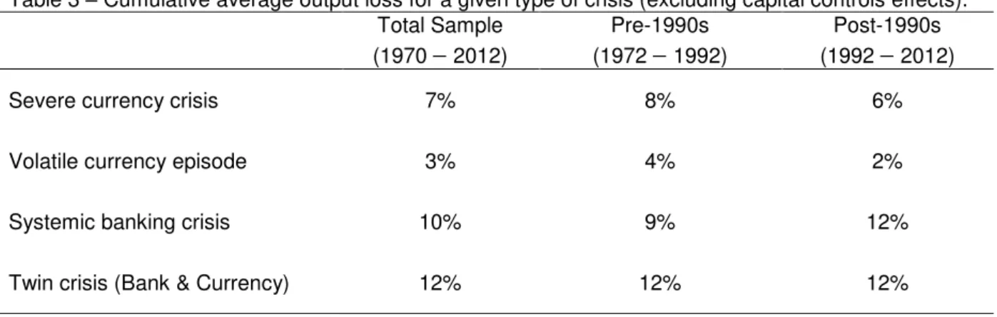
All four types of crises seem to depress output permanently irrespective of the presence of capital controls. Chart 3 and Table 3 show the impulse response of growth to crisis excluding the effect of capital controls ( =0).
Chart 3 – Impulse response of crisis on output
Severe currency crisis Volatile currency episode
Systemic banking crisis Twin crisis
Source : Author’s calculations
were more predominantly floating which allowed for smoother macroeconomic adjustments.
However, the impact of “severe” currency crises is more than double (7%) that of currency volatility. These rarer crises (only 48 occurrences in our 40 year database) are typically linked to the sudden end of a currency peg regime and/or a sudden unexpected adjustment of the exchange rate. The disruptive event is hence more powerful.
Table 3 – Cumulative average output loss for a given type of crisis (excluding capital controls effects). Total Sample
(1970 2012) (1972 1992) Pre-1990s (1992 2012) Post-1990s
Severe currency crisis 7% 8% 6%
Volatile currency episode 3% 4% 2%
Systemic banking crisis 10% 9% 12%
Twin crisis (Bank & Currency) 12% 12% 12%
Source: Author’s calculations.
Systemic banking crises have an even greater cumulative impact on output: of the order of 10%. This is also in line with the 420% estimated in the literature (SERWA 2010). Yet contrary to currency crises, it is found that the impact of banking crises has become more severe in recent years (a cumulative 12% decline in output since the 1990s). This could be explained by the greater importance of credit and the financial sector in EMEs in this period.
Finally, the largest impact comes from the twin (banking and currency) crisis which is estimated to reach 12% or double that of a severe currency crisis.
4.2 EFFECT OF CAPITAL CONTROLS
12
Chart 4 – Impulse response of a severe foreign exchange crisis (left hand chart) and of a twin crisis (right hand chart) on output with and without capital controls during the 19922012 period.
Source: Author’s calculations.
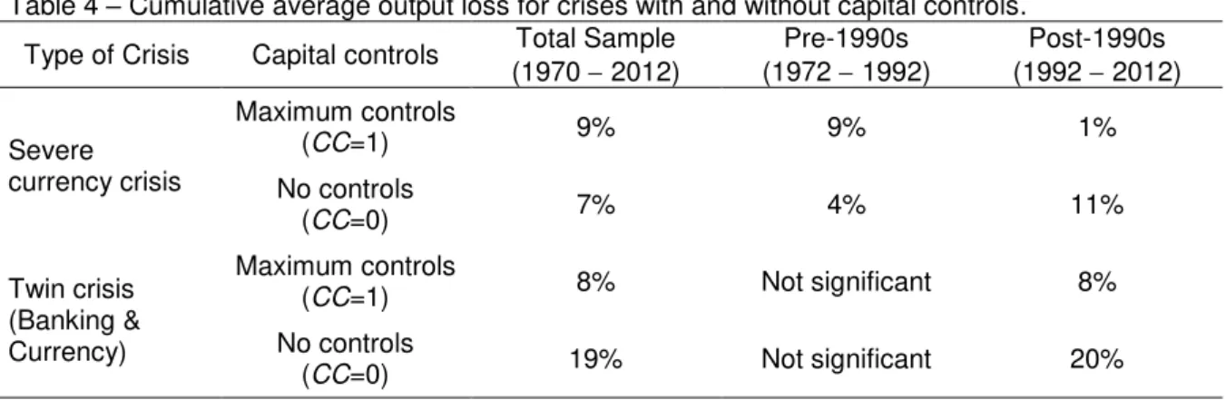
The effect of capital controls in severe currency crises is important in the post 1990s period. The existence of full controls (Ito Chinn index of 1) implied a almost insignificant decline in output, while a lack of capital controls resulted in a total cumulative GDP decline of 11%. This strong negative correlation between the existence of capital controls and the impact of currency crises observed in our results could be related to the Asian crisis where the more capital-open economies (e.g. Indonesia) suffered more than the more closed economies (e.g. Korea). However, this result is also linked to the breaking of pegs and sovereign crises in Latin America (Uruguay 1990, 2002, Argentina 2002, Brazil 1992, 1999, 2002, Venezuela 1994) where capital controls also seem to have played a dampening role.
controls (as in the case of Malaysia) made these economies and banking systems more resilient in the overall crisis.
Table 4 – Cumulative average output loss for crises with and without capital controls.
Type of Crisis Capital controls (1970 2012) Total Sample (1972 1992) Pre-1990s (1992 2012) Post-1990s
Severe
currency crisis
Maximum controls
(CC=1) 9% 9% 1%
No controls
(CC=0) 7% 4% 11%
Twin crisis (Banking & Currency)
Maximum controls
(CC=1) 8% Not significant 8%
No controls
(CC=0) 19% Not significant 20%
Source: Author’s calculations.
Note that the attenuating effect of controls does not seem to hold over the whole sample period. Table 4 and Annex C show for example that in the period 19701990, the impact of severe currency crises was twice as large when capital controls were present (9% versus 4% without controls). While for twin crisis they had an insignificant impact over this period.
4.3 FEEDBACK OF CAPITAL CONTROLS ON THE PROBABILITY OF A CRISIS
A relevant question is whether capital controls might increase the probability of a crisis even if they mitigate its impact. There is evidence that capital controls increase the chance of currency crises, particularly in the period before 1990, although the effect is insignificant for other types of crises.
To evaluate this we use a more generalised version of the probit framework proposed by Cerra and Saxena (2008). The model is augmented by including the level of capital controls ( and other variables which can also contribute to the likelihood of a crisis ( :
14
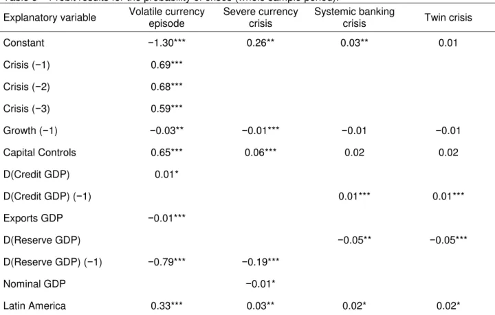
The presence of capital controls seems to be positively correlated with the probability of a crisis. Table 5 shows that coefficient for capital controls is positive and significant in both types of currency crises. This implies that it is possible that introducing capital controls can render a country more crisis-prone.
Table 5 – Probit results for the probability of crises (whole sample period).
Explanatory variable Volatile currency episode Severe currency crisis Systemic banking crisis Twin crisis
Constant −1.30*** 0.26** 0.03** 0.01
Crisis (−1) 0.69***
Crisis (−2) 0.68***
Crisis (−3) 0.59***
Growth (−1) −0.03** −0.01*** −0.01 −0.01
Capital Controls 0.65*** 0.06*** 0.02 0.02
D(Credit GDP) 0.01*
D(Credit GDP) (−1) 0.01*** 0.01***
Exports GDP −0.01***
D(Reserve GDP) −0.05** −0.05***
D(Reserve GDP) (−1) −0.79*** −0.19***
Nominal GDP −0.01*
Latin America 0.33*** 0.03** 0.02* 0.02*
***, **, * significant at the 1%, 5% and 10% level, respectively. Crisis (−1) is the crisis dummy lagged
one year, Growth is GDP growth in percent, Capital controls are controls as defined by Chinn and Ito
(2008) and rebased to range from 1 (maximum controls) to 0 (no controls), D(credit GDP) is the percentage point change of credit to private sector to GDP over the last five years, exports GDP are
the level of exports to GDP in percent, D(Reserve GDP) is the first difference of the log of reserves to
GDP, Nominal GDP is the log of nominal US$ GDP, Latin America is a dummy for a country in Latin
America.
Source: Author’s calculations.
A number of other factors, such as the level of reserves, credit growth, the geographical location (countries in Latin America, for example) and the openness of the economy are also correlated to the likelihood of a crisis (see Table 5).
4.4 ENDOGENEITY
Equation (2) also allows us to answer the question of whether crises are exogenous to growth. Table 5 shows that severe or moderate currency crises are negatively correlated to the growth rate of the previous year, so that lower growth could itself increase the probability of a crisis in the coming year. As Cerra and Saxena (2008) point out, with crises being endogenous to growth, this means that the crises coefficients in our benchmark models (Equation (1)) are probably underestimated. We find no signs of endogeneity for banking or twin crises.
Another reverse causality concern is whether capital controls are linked to growth or resilience to crises, i.e., if controls rise when growth is high or when the economy is more resilient to crises. We tackle this by including instrumental variables which are correlated to capital controls but not growth. As in Ostry et al. (2012), we use a dummy for membership of the Eurozone or the existence of a bilateral investment treaty (BIT) between each country and the US as instruments. Both agreements required the signatory countries to reduce capital controls but should not affect the resilience of growth to crises.
The results are inconclusive in the case of twin crises as there was only one occurrence of a country, member of the EU or with a BIT, suffering this type of crises. In the case of severe currency crises, Appendix F shows that the presence of capital controls increased the impact of a crisis giving us the opposite result to those
16
4.5 OMITTED VARIABLES
It is conceivable that other variables (such as credit growth, terms of trade, trade openness) could determine growth and the resilience to a crisis. If we do not test for their inclusion, the impact of the crisis on growth and capital controls could be overestimated. To do this, we include these new variables ( in Equation (1):
∑ ∑
∑
∑
5 CONCLUSION AND DISCUSSION
We find evidence that crises have significant and permanent impact on growth. Yet, higher capital controls seem to cushion some of this impact in the case of severe currency and twin crises.
Of the four types of crises reviewed in this paper (severe, and moderate foreign exchange crises, banking crises, and twin crises), the ones which include the financial sector (banking and twin crises) have the most persistent and negative impact on growth (in the order of 10 percentage points).
However, when capital controls are included as explanatory variables, results show that over the last two decades tighter capital controls policies are associated with significantly lower cumulative output loss from severe currency and
“twin” (currency and banking) crises. While the cumulative impact of each of these
crises is significant (in the order of 712%), this effect was sharply reduced in the presence of capital controls. However, I also find that this relationship was not present in the period 19701990. This might suggest that the period of higher capital inflows was also associated with a higher need for capital controls.
Yet the case for capital controls is not clear-cut. When we explore endogeneity issues, such as whether capital controls or lower growth can in turn increase the likelihood of a crisis, our probit model suggest that the presence of capital controls are positively correlated with currency crises. As this implies that more controls could make a country more crisis-prone, it suggests that cost and benefits must be carefully examined before putting these measures into place. Moreover, there is weak evidence that the results might be affected by endogeneity.
18
BIBLIOGRAPHY
BENIGNO, G., CHEN, H., OTROK, C., REBUCCI, A. AND E. YOUNG (2010),
“Revisiting Overborrowing and its Policy Implications”. CEPR Discussion Paper no.
7872. London, Centre for Economic Policy Research.
BIANCHI, J. (2011), "Overborrowing and Systemic Externalities in the Business Cycle.”, American Economic Review 101(7), pp. 3400-3426.
BUSSIERE, M.; SAXENA, S. C. AND C. E. TOVAR (2012); “Chronicle of currency collapses: Reexamining the effects on output.”Journal of International Money and Finance, v. 31, p. 680-708.
CERRA, V. AND S. C: SAXENA (2008), “The Myth of Economic Recovery.”The American Economic Review, v. 98, n. 1, p. 439-457, 2008.
CHINN, M. AND H. ITO (2008), “A new measure of financial openness.”Journal of Comparative Policy Analysis, 10 (3), 309–322.
EICHENGREEN, B. AND D. LEBLANG (2002), “Capital Account Liberalization: Was Mr. Mahathir Right?”, NBER Working Paper 9427.
FURCERI, D. AND A. MOUROUGANE (2012), “The effect of financial crises on potential output: New empirical evidence from OECD countries.” Journal of Macroeconomics, Volume 34, Issue 3, Pages 822–832.
GUPTA, P., MISHRA, D. AND R. SAHAY, (2007), “Behaviour of output during currency crises.”Journal of International Economics, 72 (2), 428–450.
INTERNATIONAL MONETARY FUND (2012), “The Liberalization and Management of Capital Flows: An Institutional View”,
http://www.imf.org/external/np/pp/eng/2012/111412.pdf.
INTERNATIONAL MONETARY FUND (2013), “World Economic Outlook Database
-April 2013”, http://www.imf.org/external/pubs/ft/weo/2013/01/weodata/index.aspx. JEANNE, O. AND A. KORINEK (2011), “Excessive Volatility in Capital Flows: A Pigouvian Taxation Approach”. American Economic Review Papers and Proceedings 100(2) pp. 403-407.
KORINEK, A. (2009), “Systemic Risk-Taking: Accelerator Effects, Externalities, and Regulatory.” Mimeo, University of Maryland.
LAEVEN, L. AND F. VALENCIA (2008), “Systemic Banking Crises: A New Database.” IMF Working Paper No. 08/224.
LORENZONI, G. (2008), “Inefficient Credit Booms.” Review of Economic Studies,
75, pp. 809-833.
MAGUD, N. E. REINHART, C. M. AND K. S. ROGOFF, K.S. (2006), “Capital controls: Myth and reality – A portfolio balance approach.”Mimeo, Harvard
University.
MISHKIN, F. (1999) “Lessons from the Asian Crisis.”Journal of International Money and Finance, 18 (4), 709-723.
OBSTFELD, M. AND K. ROGOFF, (1996) “Foundations of International Macroeconomics.” Cambridge, Massachusetts: MIT Press.
OSTRY, J. D., GHOSH, A. R., HABERMEIER, K.,CHAMON, M., QURESHI, M. S. AND D. B. S. REINHARDT, (2010), “Capital Inflows: The Role of Controls.” IMF Staff Position Note 10/04 (Washington, DC: International Monetary Fund).
OSTRY, J. D. GHOSH, A. R. CHAMON, M. AND M. S. QURESHI (2012),“Tools for
managing financial-stability risks from capital inflows.”Journal of International Economics, Doi: 10.1016/j.jinteco.2012.02.002.
QUINN, D.P., TOYODA, A.M., 2008. “Does capital account liberalization lead to economic growth?”Review of Financial Studies, 21 (3), 1403–1449.
REINHART, V. AND C. REINHART (2008), “Capital Flow Bonanzas: An
Encompassing View of the Past and Present.”CEPR Discussion Paper no. 6996.
London, Centre for Economic Policy Research.
REINHART, C. AND K. S. ROGOFF (2009), “This Time It’s Different: Eight Centuries
of Financial Folly.” Princeton, Princeton University Press.
ROMER, C. D.; AND ROMER, D. H. (1989), “Does Monetary Policy Matter? A New Test in the Spirit of Friedman and Schwartz”, NBER Macroeconomics Annual, v. 4,
p. 121-70.
SCHINDLER, M. (2009), “Measuring financial integration: a new data set.”IMF Staff Papers 56 (1), 222–238.
SERWA, D. (2010), “Larger crises cost more: Impact of banking sector instability on
output growth.”Journal of International Money and Finance, 29, 1463-1481. WORLD BANK (2013), “World Development Indicators 2013”,
20
APPENDIX A – DATA SOURCES
Data sources for variables used in the analysis.
Variable Description Source
Growth rate Annual GDP growth rate 1970-79 World Bank (2013) & 1980-2012 IMF (2013).
Volatile currency
episode Dummy for currency crisis as defined by Reinhart and Rogoff (2009)2
1970-2010 Reinhart and Rogoff (2009) & 2011-12 Laeven and Valencia (2012) Severe currency
crisis Dummy for currency crisis as defined by Laeven and Valencia (2012) Laeven and Valencia (2012) Systemic banking
crisis Dummy for first year of systemic banking crisis as defined by Laeven and Valencia (2012) Laeven and Valencia (2012)
Twin crisis
Dummy for first year of banking crisis (Laeven and Valencia (2012)) simultaneously with a volatile currency episode (Reinhart and Rogoff (2009)).
Reinhart and Rogoff (2009) & Laeven and Valencia (2012)
Capital Controls rebased to range from 1 (maximum controls) to 0 Controls as defined by Chinn and Ito (2008) and (no controls).
Chinn and Ito (2008)
GDP per capita Log of GDP per capita (not PPP adjusted) World Bank (2013)
Reserves GDP Log of total reserves (including gold) to nominal GDP World Bank (2013)
Credit GDP Domestic credit to private sector to GDP (percent) World Bank (2013)
Exports GDP Exports to GDP (percent) World Bank (2013)
Terms of Trade Net barter terms of trade year on year change (percent) World Bank (2013)
Debt GDP Total gross central government debt to GDP Reinhart and Rogoff (2009)
External Debt
GDP Total (private and public) external debt to GDP Reinhart and Rogoff (2009) Source: Author’s calculations.
2
APPENDIX B – PANEL ESTIMATION RESULTS FOR CRISES IMPACT ON OUTPUT (EXCLUDING CAPITAL CONTROLS EFFECTS)
Estimation results for crisis impact on output.
Explanatory variable
Volatile currency
episode
Severe
currency crisis banking crisis Systemic Twin crisis
Full sample period
Constant 3.74*** 2.48*** 2.52*** 2.42***
Growth (−1) 0.31*** 0.37*** 0.34*** 0.32***
Crisis −1.80*** −4.47*** −2.99*** −3.95***
Crisis (−1) −0.60* −4.31*** −4.92***
19721992 period
Constant 4.59*** 2.40*** 2.07*** 2.42***
Growth (−1) 0.23*** 0.27*** 0.27*** 0.27***
Crisis −2.04*** −3.21*** −3.45*** −5.55***
Crisis (−1) −1.12*** −2.58*** −3.25*** −3.75*** 19922012 period
Constant −3.07*** 2.36** 3.91*** 3.11***
Growth (−1) 0.38*** 0.44*** 0.35*** 0.32***
Crisis −1.59*** −6.29*** −2.92*** −2.74***
Crisis (−1) 2.92** −5.18*** −5.66***
Notes: ***, **, * significant at the 1%, 5% and 10% level respectively. Crisis (−1) is the crisis dummy
lagged one year, Growth is GDP growth in percent. To save space time and individual (fixed effects)
dummies not shown but were included and were significant in all versions of the model. Numbers rounded to 2 decimal places.
22
APPENDIX C – PANEL ESTIMATION RESULTS FOR CRISES IMPACT ON OUTPUT (WITH CAPITAL CONTROLS EFFECTS)
Estimation results for crisis impact on output.
Explanatory variable Severe currency crisis Twin crisis
Full sample period
Constant 3.15*** 2.81***
Growth (−1) 0.28*** 0.27***
Crisis −4.77*** −4.15***
Crisis (−1) −11.10***
Capital Controls
Capital Controls (−1) −1.75** 8.79***
19721992 period
Constant 2.59***
Growth (−1) 0.24***
Crisis −3.21***
Crisis (−1)
Capital Controls
Capital Controls (−1) −4.08*** 19922012 period
Constant 3.79*** 3.01***
Growth (−1) 0.31*** 0.25***
Crisis −11.51*** −3.10**
Crisis (−1) 2.28** −13.39***
Crisis (−2) 1.60**
Capital Controls 7.38***
Capital Controls (−1) −10.44***
Notes: ***, **, * significant at the 1%, 5% and 10% level respectively. Crisis (−1) is the crisis dummy
lagged one year, Growth is GDP growth in percent. Capital controls are controls as defined by Chinn
and Ito (2008) and rebased to range from 1 (maximum controls) to 0 (no controls). To save space time and individual (fixed effects) dummies not shown but were included and were significant in all versions of the model. Numbers rounded to 2 decimal places.
APPENDIX D – PROBIT RESULTS FOR PROBABILITY OF CRISIS ESTIMATED FOR 1992-2012 PERIOD
Probit results for the probability of crises (1992-2012 period).
Explanatory variable Volatile currency episode Severe currency crisis banking crisis Systemic Twin crisis
Constant −0.01 0.04*** 0.02 0.01
Crisis (−1) 0.21***
Crisis (−2) 0.16***
Crisis (−3) 0.08*
Growth (−1) 0.01 −0.01*** −0.01 −0.01
Capital Controls 0.13*** 0.07*** 0.03 0.03
D(Credit GDP) 0.01*
D(Credit GDP) (−1) 0.01*** 0.01***
Exports GDP −0.01***
D(Reserve GDP) −0.19** −0.10*** −0.08***
D(Reserve GDP) (−1) −0.18***
Terms of Trade (−1) −0.01** −0.01**
Latin America 0.08**
***, **, * significant at the 1%, 5% and 10% level respectively. Crisis (−1) is the crisis dummy lagged
one year, Growth is GDP growth in percent, Capital controls are controls as defined by Chinn and Ito
(2008) and rebased to range from 1 (maximum controls) to 0 (no controls), D(credit GDP) is the
percentage point change of credit to private sector to GDP over the last 5 years, exports GDP are the
level of exports to GDP in percent, D(Reserve GDP) is the first difference of the log of reserves to GDP, Nominal GDP is the log of nominal US$ GDP, Latin America is a dummy for a country in Latin
America, Terms of Trade is terms of trade year on year change in percent.
24
APPENDIX E – PANEL ESTIMATION RESULTS FOR CRISES IMPACT ON OUTPUT WITH ADDITIONAL EXPLANATORY VARIABLES (TO CONTROL FOR OMMITTED VARIABLES).
Estimation results for crisis impact on output.
Explanatory variable Volatile currency episode Severe currency crisis Systemic banking crisis Twin crisis
Full sample period
Constant 3.44*** 3.40*** 2.81*** 3.86***
Growth (−1) 0.27*** 0.25*** 0.32*** 0.20***
Crisis −1.77*** −4.92*** −2.82*** −3.97***
Crisis (−1) −0.83** −3.98*** −11.13***
Capital control
Capital control (−1) −2.04*** 9.49***
Exports GDP 0.07*** 0.01 0.02
Reserve GDP 0.76**
Credit GDP −0.02** −0.02*** −0.02** −0.02**
Debt GDP −0.03***
19721992 period
Constant 9.39 3.03*** 2.40*** 2.65***
Growth (−1) 0.14** 0.18*** 0.21*** 0.22***
Crisis −1.70*** −3.17*** −3.04*** −4.85***
Crisis (−1) −1.15*** −3.43*** −2.37***
Capital control
Capital control (−1) −4.53***
GDP per capita 1.78*
Exports GDP 0.07*** 0.05** 0.05** 0.04**
Reserve GDP (−1) 2.49***
Credit GDP −0.05***
D (Credit GDP) −0.03* −0.03* −0.03*
19922012 period
Constant 4.92*** 5.25*** 4.67*** 3.78***
Growth (−1) 0.22*** 0.16*** 0.17*** 0.14**
Crisis −1.27*** −10.13*** −3.10*** −1.62*
Crisis (−1) −4.63*** −9.42***
Capital control 5.15**
Capital control (−1) 7.24***
D (Reserve GDP) −2.10*** 3.30***
D (Reserve GDP) (−1) 4.09*** 3.03***
Credit GDP −0.04***
D (External Debt GDP) −0.03*** −0.04***
Terms of Trade 0.04* 0.03*
Terms of Trade (−1) 0.06*** 0.05*** 0.06***
Notes: ***, **, * significant at the 1%, 5% and 10% level respectively. Crisis is the crisis dummy, Growth is GDP growth in percent. GDP per capita is log of GDP per capita. Reserve GDP is log of
total foreign currency reserves to GDP. D(Reserves GDP) is the percentage point year on year
change of Reserves GDP. Credit GDP is domestic credit to private sector to GDP in percent. D(Credit GDP) is the 5 year percentage point change of Credit GDP over the previous 5 years. Debt GDP is
the total gross central government debt to GDP in percent. D(External Debt GDP) is the 3 year
percentage point change of total (public and private) external debt to GDP.Terms of trade is year on
year percent change in the net barter terms of trade. All variables with (−1) are lagged by one year.
To save space, time and individual dummies are not shown but were included and were significant in all versions of the model. Numbers rounded to 2 decimal places.
APPENDIX F – PANEL ESTIMATION RESULTS FOR CRISES IMPACT ON OUTPUT WITH INSTRUMENTAL VARIABLES TO CONTROL FOR ENDOGENEITY OF CAPITAL CONTROLS AND CRISIS RESILIENCE
Estimation results for crisis impact on outputa)
Explanatory variable Severe currency crisis Twin crisis
Full sample period
Constant 0.74* 0.59
Growth (−1) 0.33*** 0.44***
Crisis −1.70*** −0.05
Crisis (−1) −1.15
Capital Controls
Capital Controls (−1) −1.13** 0.70
19922012 period
Constant 2.65*** 2.36***
Growth (−1) 0.35*** 0.42***
Crisis −3.41*** 0.12
Crisis (−1) 0.31* −2.35***
Crisis (−2) 0.73**
Capital Controls −2.52***
Capital Controls (−1) −1.70**
Notes: ***, **, * significant at the 1%, 5% and 10% level respectively. Crisis (−1) is the crisis dummy
lagged one year, Growth is GDP growth in percent. Capital controls are controls as defined by Chinn
and Ito (2008) and rebased to range from 1 (maximum controls) to 0 (no controls). To save space time and individual (fixed effects) dummies not shown but were included and were significant in all versions of the model. Numbers rounded to 2 decimal places.
a)1970
−90 period not tested as none of the emerging markets in this sample were EU members or were signatories of a US Bilateral Investement Treaty in this period.
26
APPENDIX G – LIST OF ECONOMIES IN OUR ANALYSIS
Economies used in the analysis.
Latin America East Europe, Middle East and Africa Asia
Argentina Czech Republic China
Brazil Hungary Hong Kong
Chile Israel Indonesia
Colombia Poland India
Ecuador Romania South Korea
Mexico Russian Federation Malaysia
Peru Turkey Singapore
Uruguay South Africa Thailand
Venezuela Ukraine