Outubro de 2014
Working
Paper
370
Do capital controls boost EME´s
resilience to financial crises
?
TEXTO PARA DISCUSSÃO 370•OUTUBRO DE 2014• 1
Os artigos dos Textos para Discussão da Escola de Economia de São Paulo da Fundação Getulio Vargas são de inteira responsabilidade dos autores e não refletem necessariamente a opinião da
FGV-EESP. É permitida a reprodução total ou parcial dos artigos, desde que creditada a fonte.
Escola de Economia de São Paulo da Fundação Getulio Vargas FGV-EESP
Roman Goossens Graduate Institute, Geneva
Rogerio Mori
Sao Paulo School of Economics – FGV
Vladimir K. Teles1
Sao Paulo School of Economics – FGV
ABSTRACT
Capital controls are again in vogue as a number of emerging markets have reintroduced these measures in recent years in response to a “flood” of international capital. Policymakers use these tools to buttress their economies against the “sudden stop” risk that accompanies international capital flows. Using a panel VAR model, we show that capital controls appear to make emerging market economies (EMEs) more resistant to financial crises by showing that lower post-crisis output loss is correlated with stronger capital controls. However, EMEs that employ capital controls seem to be more crisis-prone. Thus, policymakers should carefully evaluate whether the benefits of capital controls outweigh their costs.
Keywords: Emerging Market Economies, Capital Controls, Crises.
1
1 INTRODUCTION
Do capital controls help or hurt emerging countries that are recovering from financial crises? Can such regulations help countries avoid financial crises in the first place? In this article, we attempt to answer these questions by examining data from an annual panel of 26 emerging countries for the 1970–2012 period.
Following the 2008 crisis, many emerging countries significantly increased their use of capital controls to prevent so-called "sudden-stop" episodes, but it is not clear whether capital controls are effective in addressing this problem. Although a number of studies have attempted to ascertain whether capital controls reduce capital flows or affect the exchange rate (see Magud, Reinhart and Rogoff (2011) and Ostry et al. (2010) for a survey), few studies have explored whether these measures affect the resilience of emerging market economies (EMEs) to financial crises. This question is particularly relevant given the evidence that financial crises have a persistent impact on economic growth (e.g., Furceri and Mourougane (2012)). This paper attempts to fill this gap in the literature by estimating whether the decline in the long-run level of output following a financial crisis depends on the level of capital controls. We examine four types of crises in this paper: severe foreign exchange (FX) crises, moderate FX crises, banking crises and twin (FX and banking) crises.
Our paper aims to empirically quantify the longer-term impact of capital controls on output and merges two separate questions posed in two different streams of the literature: the first seeks to estimate the recent short-term effects of capital controls on recovery from the 2008 crisis (Ostry et al., 2012) and the second attempts to evaluate the long-term impact of financial crises on growth (Cerra and Saxena, 2008).
Ostry et al. (2012) construct a measure of controls on capital inflows to estimate the resilience of EME growth to the 2008 crisis but only measure the correlation between capital inflow controls on economic recovery in the year following the crisis. In the current paper, we attempt to determine the effects of capital controls several years following crises and to explore the overall impact of controls on capital inflows and outflows.
dataset covering a longer period and ask whether capital controls affect the persistence of such crises.
Bussière, Saxena and Tovar (2012) use a similar model with a larger dataset that spans 20 years but does not include the 2008 crisis. These authors find that a currency crisis leads to a long-term 2% to 6% decline in output three years following the end of the crisis. However, these authors also fail to ask whether capital controls might have a stabilizing influence.
In our analysis, we employ data from 26 major emerging markets during the 1970–2012 period and an unbalanced fixed-effects panel regression; we find that all crises depress output permanently. However, we also show that output losses following certain types of crises in recent years (“severe” exchange-rate and twin crises) have been notably lower when capital controls were tighter. In some cases, the impact of a crisis was nearly non-existent when controls were in place. Nonetheless, evidence that capital controls are linked to a higher likelihood of currency crises suggests that they might make EMEs even more crisis-prone.
Our results are robust to the inclusion of other explanatory variables of crises (including the level of debt, reserves, terms of trade, etc.). We also examine endogeneity issues, such as whether capital controls or lower growth can in turn increase the likelihood of a crisis.
2 METHODOLOGY
This paper uses a panel fixed-effects VAR (similar to that found in Cerra and Saxena (2008)) to analyze the impulse response function of emerging market growth to crises. The main purpose of the analysis is to estimate the impact of crises on the level of growth with and without capital controls.
The following benchmark specification (based on Cerra and Saxena 2008) is estimated as a dynamic panel.
∑ ∑
where is the rate of GDP growth, is a crisis dummy variable (equal to 1 if there is a FX, banking or twin crisis) and is a measure of capital controls (1 equals maximum capital restriction). The interaction term represents the level of capital controls during a crisis. We test for significance to determine whether capital controls have a dampening impact on the output that is lost during a crisis. Time and individual dummies are included to control for differentiated average growth rates among countries and over time.
2.1 DATA AND CRISES DEFINITIONS
This study employs annual data from 1970 to 2012 for 26 major EMEs (see Appendix G). GDP data come from the World Bank database (before 1980) and the IMF WEO database (1980 and later).
The estimates use four types of crisis dummies: “severe” FX volatility, moderate FX volatility, banking crises and twin crises:
1. Severe FX crises, as defined by Laevan and Valencia (2012), are more
potent (typically involving the end of an exchange-rate peg regime) and have a clearer impact on growth.
2. FX volatility episodes are another set of less stringent dummy for FX
crises. As the literature also defines currency crises as episodes of heightened FX volatility, we also define a crisis as any yearly depreciation greater than 15% against the US dollar (Reinhart and Rogoff (2009)). 3. Bank crises are defined as the first year of a systemic bank crisis (LAEVAN
AND VALENCIA (2012)), given the difficulty of dating the exact ending of banking crises (as in Cerra and Saxena (2008)).
4. Twin crises are defined as a dummy which equals one if it is the first year
of a systemic bank crisis combined with an episode of FX volatility.
We measure the level of capital control following Chinn and Ito (2008) because this measure has the longest span (it begins in the 1970s and is updated to 2011) and is available for most countries (covering 182 developed and developing economies). The series measures the extent of capital account openness based on
(AREAER). The data are renormalized to fall within the range of 1 (maximum controls) to 0 (no controls).
The drawback of this series is that it does not differentiate among the different forms of inflow and outflow controls. However, this dataset is preferred to the other widely used capital controls series (e.g., SCHINDLER (2009), QUINN AND TOYODA (2008)) because these latter series do not cover a large enough timespan, they only date back to the mid-1990s.
Other data (like credit to GDP, foreign reserves, terms of trade) that are used in the latter part of the analysis are taken from a number of sources, as detailed in Appendix A.
2.2 DATA DESCRIPTION
Figure 1 shows the trends in terms of growth, crises and capital controls in selected EMEs since the 1970s.
The top-right figure shows that there was a monotonic declining trend in
EME growth from 1970 to 2000, a sharp pickuop until the 2008 crisis but then a
renewed decline in recent years. EME GDP growth rates fell by nearly half from the 1970s to the 1990s (from approximately 6% to 3%), which likely was a consequence of financial crises that characterize much of the 1980s and 1990s. After 2000, growth reaccelerated, but in the five years following the 2008 global financial crisis, this has again reversed and growth has returned to the 1990s level.
The bottom-right figure shows clearly how crisis have tended to
Figure 1 – Trends in terms of growth, crises and capital controls in selected EMEs since the 1970s.
Five-year average EME GDP growtha) Average EME capital controls indexb)
FX volatility episodesc) Bank, Severe FX and Twin crisesc)
Source: Author’s calculations, Chinn and Ito (2008), World Bank (2013), IMF (2013), Laevan and Valencia (2012), Reinhart and Rogoff (2009).
a) Simple average of five-year GDP growth in emerging markets in percent; b) Simple average Chinn
and Ito capital controls index (1=maximum controls, 0=minimum controls). c) Proportion of countries experiencing crises (five-year average).
The trend in capital controls is somewhat different; controls were broadly stable until the 1990’s. However, since that time, as financial liberalization advanced internationally, capital controls have experienced a trend decline and are presently on average at around half the level of the 1980s.
Throughout our study we separate our sample into two periods to capture the financial liberalization of the 1990s. Table 1 summarizes the trends highlighted above: post-1990s EMEs had lower capital controls, experienced lower growth and faced somewhat fewer crises (although this is clearest in the case of FX volatility episodes). 0.0 1.0 2.0 3.0 4.0 5.0 6.0 7.0
1970 1980 1990 2000 2010
0.2 0.3 0.4 0.5 0.6 0.7 0.8
1970 1980 1990 2000 2010
0% 10% 20% 30% 40% 50% 60%
1970 1980 1990 2000 2010
0% 2% 4% 6% 8% 10% 12%
1970 1980 1990 2000 2010
Table 1 – Descriptive statistics.
Total Sample (19702012)
Pre-1990s (19701991)
Post-1990s (19922012)
Number of countries 26 23 26
Average growth rate 4.3 4.6 4.0
Average level of controls 0.53 0.61 0.45
Total Number of Crises years 336 210 126
Severe FX Crises 48 28 20
FX volatility episodes 317 199 118
Banking Crises 36 19 17
Twin Crises 23 11 12
Source: Author’s calculations, Chinn and Ito (2008), World Bank (2013), IMF (2013), Laevan and Valencia (2012), Reinhart and Rogoff (2009).
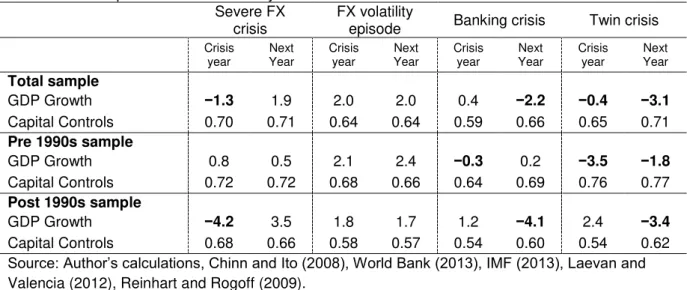
Finally, when focusing exclusively on crisis episodes (Table 2), we note that the strongest effects on growth come from twin and banking crises, which is supported in the empirical analysis in the next section.
Table 2 – Descriptive statistics in crisis years. Severe FX
crisis FX volatility episode Banking crisis Twin crisis
Crisis
year Year Next Crisis year Year Next Crisis year Next Year Crisis year Year Next
Total sample
GDP Growth −1.3 1.9 2.0 2.0 0.4 −2.2 −0.4 −3.1 Capital Controls 0.70 0.71 0.64 0.64 0.59 0.66 0.65 0.71 Pre 1990s sample
GDP Growth 0.8 0.5 2.1 2.4 −0.3 0.2 −3.5 −1.8
Capital Controls 0.72 0.72 0.68 0.66 0.64 0.69 0.76 0.77 Post 1990s sample
GDP Growth −4.2 3.5 1.8 1.7 1.2 −4.1 2.4 −3.4
Capital Controls 0.68 0.66 0.58 0.57 0.54 0.60 0.54 0.62 Source: Author’s calculations, Chinn and Ito (2008), World Bank (2013), IMF (2013), Laevan and Valencia (2012), Reinhart and Rogoff (2009).
3 RESULTS
the period of higher capital inflows was also associated with a higher need for capital controls.
3.1 EFFECT OF CRISES ON OUTPUT
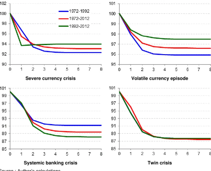
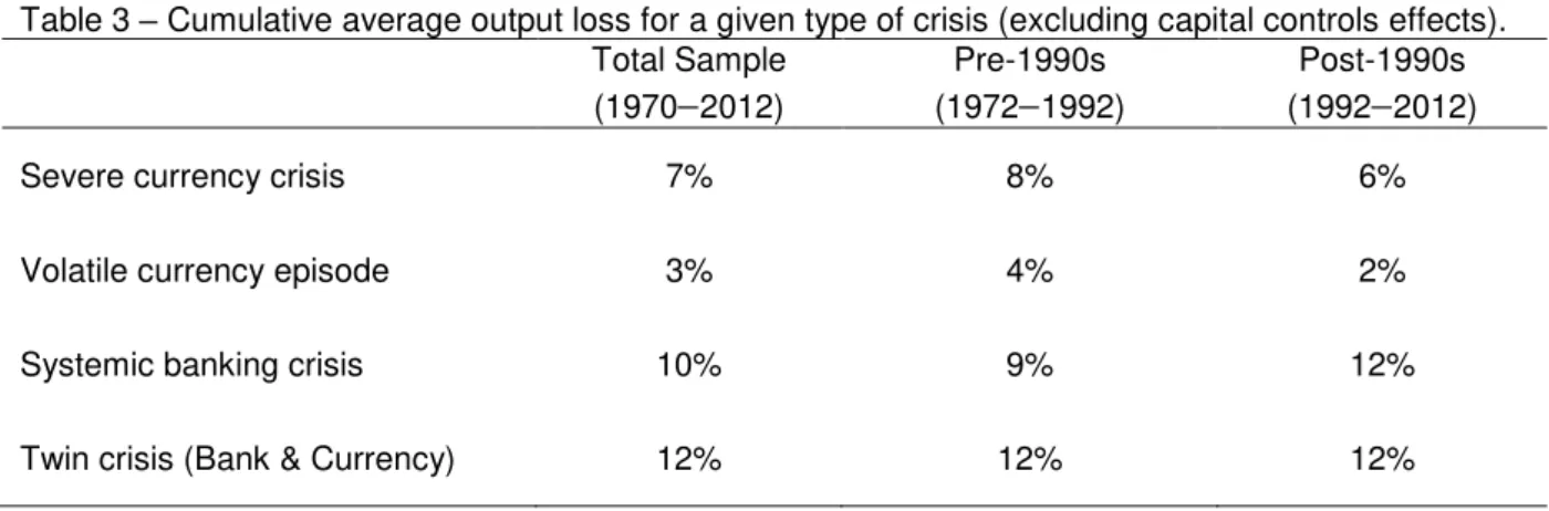
All four types of crisis seem to depress output permanently, without regard to the presence of capital controls. Figure 2 and Table 3 show the impulse response of growth to crisis excluding the effect of capital controls ( =0).
Figure 2 – Impulse response of crisis on output
Severe currency crisis Volatile currency episode
Systemic banking crisis Twin crisis Source : Author’s calculations
in recent years, with our estimate for output loss at 2% for the period after 1990. This decline is consistent with improved EME fundamentals and the fact that exchange rates were more likely to be floating during this period, which allows for smoother macroeconomic adjustments.
However, the impact of “severe” currency crises is more than double (7%) that of currency volatility. These rarer crises (only 48 occurrences in our 40-year database) are typically linked to the sudden end of a currency peg regime and/or a sudden and unexpected adjustment of the exchange rate, which makes the disruptive event more powerful.
Table 3 – Cumulative average output loss for a given type of crisis (excluding capital controls effects). Total Sample
(19702012)
Pre-1990s (19721992)
Post-1990s (19922012)
Severe currency crisis 7% 8% 6%
Volatile currency episode 3% 4% 2%
Systemic banking crisis 10% 9% 12%
Twin crisis (Bank & Currency) 12% 12% 12%
Source: Author’s calculations.
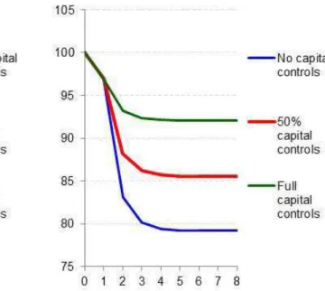
3.2 EFFECT OF CAPITAL CONTROLS
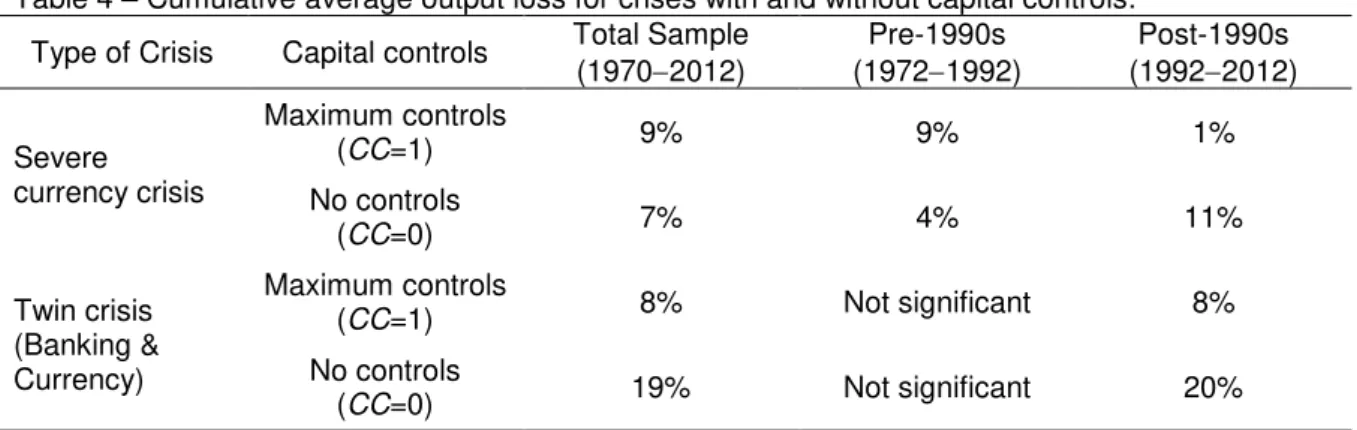
Over the last 20 years, capital controls have had a significant dampening influence on the cumulative impact of severe currency and twin crises and have reduced overall GDP loss by up to 10% (Figure 3). However, such controls did not affect the cumulative outcome of banking crises or volatile currency episodes.
It is possible that capital controls (or the absence of capital controls) affect the level of pre-crisis investment—including foreign investment—in a particular EME and, therefore, the level of pre-crisis economic growth in such EME.
This level of economic growth is important because there seems to be a natural relationship between the absence of capital controls and investment, i.e., those countries that are likely to suffer the greatest losses in an economic crisis are likely to have previously enjoyed the greatest pre-crisis gains. Because capital controls are aimed at insulating a country from negative spillover effects, they also impact the level of economic growth by restraining investment. Thus, we acknowledge that pre-crisis capital flows should be explained and analyzed before providing any policy prescription because such flows may have a direct influence on the impact of later crises.
Figure 3 – Impulse response of a severe FX crisis (left-hand figure) and of a twin crisis (right-hand figure) on output with and without capital controls during the 19922012 period.
The effect of capital controls in severe currency crises has been important since 1990. The existence of full controls (Ito Chinn renormalized index of 1) implied an almost insignificant decline in output, whereas a lack of capital controls resulted in a cumulative GDP decline of 11%. This strong negative correlation between the existence of capital controls and the impact of currency crises observed in our results might be related to the Asian crisis in which the more capital-open economies (e.g., Indonesia) suffered more than the more closed economies (e.g., Korea). However, this result may also be linked to the abandonment of currency peg regimes and various sovereign crises experienced in Latin America (Uruguay 1990, 2002, Argentina 2002, Brazil 1992, 1999, 2002, Venezuela 1994), where capital controls also seem to have played a dampening role.
The effect of capital controls on twin crises was equally substantial (over 10pp, see Table 4), although they do not manage to fully offset the crisis impact. This effect might also be linked to the Asian crisis, when sudden large depreciations sharply increased the foreign currency liabilities of some domestic banking systems and put their balance sheets under stress (Mishkin (1999)). Because the Ito Chinn capital controls indicator does not distinguish between inflow and outflow controls, it is possible that capital outflows controls (as in the case of Malaysia) made these economies and banking systems more resilient during the overall crisis.
Table 4 – Cumulative average output loss for crises with and without capital controls.
Type of Crisis Capital controls Total Sample (19702012) (1972Pre-1990s 1992) (1992Post-1990s 2012)
Severe
currency crisis
Maximum controls
(CC=1) 9% 9% 1%
No controls
(CC=0) 7% 4% 11%
Twin crisis (Banking & Currency)
Maximum controls
(CC=1) 8% Not significant 8%
No controls
(CC=0) 19% Not significant 20%
Source: Author’s calculations.
suggests that capital controls are less effective regarding such crises because the flows of international capital in these economies are not necessarily intense during such crises.
Note that the attenuating effect of controls does not seem to hold over the entire sample period. For example, Table 4 and Annex C show that the impact of severe currency crises during the 1970–1990 period was twice as large when capital controls were present (9%) than without such controls (4%), although they had an non-significant impact on twin crises during this same period.
3.3 FEEDBACK OF CAPITAL CONTROLS ON THE PROBABILITY OF A CRISIS A relevant question is whether capital controls might increase the probability of a crisis, despite mitigating the impact of a crisis. There is evidence that capital controls increase the likelihood of currency crises, particularly in the period before 1990, although the effect is non-significant for other types of crises.
To evaluate this possibility, we use a more generalized version of the probit framework proposed by Cerra and Saxena (2008). The model is augmented by including the level of capital controls ( and other variables that can contribute to the likelihood of a crisis ( :
( ) { ∑ ∑
∑ ∑
}
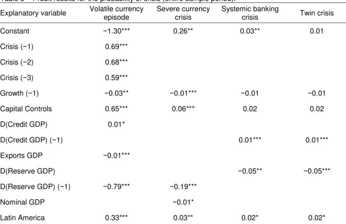
In fact, the presence of capital controls seems positively correlated with the likelihood of a crisis. Table 5 shows that the coefficient for capital controls is positive and significant in both types of currency crisis, which implies that introducing capital controls may render a country more crisis-prone. This results because governments that adopt such capital controls in these economies are attempting to control exchange rate movements. This type of control is perceived by international investors as a potential source of speculative gains as long as the exchange rate deviates from the equilibrium in some periods.
openness of the economy that are also correlated with the likelihood of a crisis (see Table 5). These relationships have remained broadly stable over the most recent 20 years, although there are signs that capital controls and growth have lost some of their significance in recent years (see Appendix D).
Table 5 – Probit results for the probability of crisis (entire sample period).
Explanatory variable Volatile currency episode Severe currency crisis Systemic banking crisis Twin crisis
Constant −1.30*** 0.26** 0.03** 0.01
Crisis (−1) 0.69***
Crisis (−2) 0.68***
Crisis (−3) 0.59***
Growth (−1) −0.03** −0.01*** −0.01 −0.01
Capital Controls 0.65*** 0.06*** 0.02 0.02
D(Credit GDP) 0.01*
D(Credit GDP) (−1) 0.01*** 0.01***
Exports GDP −0.01***
D(Reserve GDP) −0.05** −0.05***
D(Reserve GDP) (−1) −0.79*** −0.19***
Nominal GDP −0.01*
Latin America 0.33*** 0.03** 0.02* 0.02*
***, **, * denotes significance at the 1%, 5% and 10% levels, respectively. Crisis (−1) is the crisis dummy lagged one year, Growth is GDP growth expressed as a percentage, Capital controls are controls defined in Chinn and Ito (2008) and rebased to range from 1 (maximum controls) to 0 (no controls), D(credit GDP) represents the percentage point change of credit to private sector to GDP over the last five years, exports GDP represents the level of exports to GDP as a percentage, D(Reserve GDP) is the first difference of the log of reserves to GDP, Nominal GDP is the log of nominal US$ GDP, and Latin America is a dummy for a country in Latin America.
Source: Author’s calculations.
3.4 ENDOGENEITY
Another reverse causality concern is whether capital controls are linked to growth or resilience to crises, i.e., whether controls rise when growth is high or when the economy is more resilient to crisis. We address this matter by including instrumental variables that are correlated to capital controls but not growth. As in Ostry et al. (2012), we use a dummy for membership in the Eurozone or the existence of a bilateral investment treaty (BIT) between the country and the US as instruments. Both agreements require the signatory countries to reduce capital controls but should not affect the resilience of growth to crises. The results are inconclusive regarding twin crises, and there was only one country (i.e., a member of the EU or with a BIT) that suffered this type of crisis (one occurrence). In the case of severe currency crises, Appendix F shows that the presence of capital controls
increased the impact of a crisis, which is contrary to the results found in the previous
literature. Once again, given the small sample of countries that are members of the EU or that have a BIT and that suffered these crises—and given that half the episodes are concentrated in one country (Turkey), these results might be biased and should be checked against a larger dataset.
3.5 OMITTED VARIABLES
It is conceivable that other variables (such as credit growth, terms of trade, and trade openness) might determine growth and resilience to crisis. If we do not test for their inclusion, the impact of the crisis on growth and capital controls might be overestimated. To perform this test, we include these new variables in Equation (1) and we find that most of the estimations are robust to the inclusion of these additional variables (see Appendix E).
5 DISCUSSION AND CONCLUSION
We find evidence that crises have significant and permanent impacts on growth. Nonetheless, higher capital controls seem to cushion some of this impact in the case of severe currency and twin crises.
However, when capital controls are included as explanatory variables, the results from the most recent two decades indicate that tighter capital control policies are associated with significantly lower cumulative output loss from severe currency and twin crises. Although the cumulative impact of each of these types of crises is significant (on the order of 712%), this effect was sharply reduced in the presence of capital controls. However, we also find that this relationship was not present during the 19701990 period, which might suggest that the period of higher capital inflows was also associated with a higher need for capital controls.
BIBLIOGRAPHY
BENIGNO, G., CHEN, H., OTROK, C., REBUCCI, A. AND E. YOUNG (2010),
“Revisiting Overborrowing and its Policy Implications”. CEPR Discussion Paper no.
7872. London, Centre for Economic Policy Research.
BIANCHI, J. (2011), "Overborrowing and Systemic Externalities in the Business
Cycle.”, American Economic Review 101(7), pp. 3400-3426.
BUSSIERE, M.; SAXENA, S. C. AND C. E. TOVAR (2012); “Chronicle of currency collapses: Reexamining the effects on output.”Journal of International Money and Finance, v. 31, p. 680-708.
CERRA, V. AND S. C: SAXENA (2008), “The Myth of Economic Recovery.”The American Economic Review, v. 98, n. 1, p. 439-457, 2008.
CHINN, M. AND H. ITO (2008), “A new measure of financial openness.” Journal of Comparative Policy Analysis, 10 (3), 309–322.
EICHENGREEN, B. AND D. LEBLANG (2002), “Capital Account Liberalization: Was
Mr. Mahathir Right?”, NBER Working Paper 9427.
FURCERI, D. AND A. MOUROUGANE (2012), “The effect of financial crises on potential output: New empirical evidence from OECD countries.” Journal of Macroeconomics, Volume 34, Issue 3, Pages 822–832.
GUPTA, P., MISHRA, D. AND R. SAHAY, (2007), “Behaviour of output during
currency crises.” Journal of International Economics, 72 (2), 428–450.
INTERNATIONAL MONETARY FUND (2012), “The Liberalization and Management of Capital Flows: An Institutional View”,
http://www.imf.org/external/np/pp/eng/2012/111412.pdf.
INTERNATIONAL MONETARY FUND (2013), “World Economic Outlook Database
-April 2013”, http://www.imf.org/external/pubs/ft/weo/2013/01/weodata/index.aspx.
JEANNE, O. AND A. KORINEK (2011), “Excessive Volatility in Capital Flows: A
Pigouvian Taxation Approach”. American Economic Review Papers and
Proceedings 100(2) pp. 403-407.
KLEIN, Michael; OLIVEI, Giovanni (2008) Capital account liberalization, financial depth, and economic growth. Journal of International Money and Finance Volume 27, Issue 6, October 2008, Pages 861–875
KORINEK, A. (2009), “Systemic Risk-Taking: Accelerator Effects, Externalities, and Regulatory.” Mimeo, University of Maryland.
LAEVEN, L. AND F. VALENCIA (2008), “Systemic Banking Crises: A New
LAEVEN, L. AND F. VALENCIA (2012), “Systemic Banking Crises: An Update.” IMF Working Paper No. 12/163.
LORENZONI, G. (2008), “Inefficient Credit Booms.” Review of Economic Studies,
75, pp. 809-833.
MAGUD, N. E. REINHART, C. M. AND K. S. ROGOFF, K.S. (2006), “Capital controls: Myth and reality – A portfolio balance approach.”Mimeo, Harvard University.
MISHKIN, F. (1999) “Lessons from the Asian Crisis.” Journal of International
Money and Finance, 18 (4), 709-723.
OBSTFELD, M. AND K. ROGOFF, (1996) “Foundations of International
Macroeconomics.” Cambridge, Massachusetts: MIT Press.
OSTRY, J. D., GHOSH, A. R., HABERMEIER, K.,CHAMON, M., QURESHI, M. S. AND D. B. S. REINHARDT, (2010), “Capital Inflows: The Role of Controls.” IMF Staff Position Note 10/04 (Washington, DC: International Monetary Fund).
OSTRY, J. D. GHOSH, A. R. CHAMON, M. AND M. S. QURESHI (2012),“Tools for
managing financial-stability risks from capital inflows.”Journal of International
Economics, Doi: 10.1016/j.jinteco.2012.02.002.
QUINN, D.P., TOYODA, A.M., 2008. “Does capital account liberalization lead to
economic growth?” Review of Financial Studies, 21 (3), 1403–1449.
REINHART, V. AND C. REINHART (2008), “Capital Flow Bonanzas: An
Encompassing View of the Past and Present.”CEPR Discussion Paper no. 6996. London, Centre for Economic Policy Research.
REINHART, C. AND K. S. ROGOFF (2009), “This Time It’s Different: Eight Centuries of Financial Folly.” Princeton, Princeton University Press.
ROMER, C. D.; AND ROMER, D. H. (1989), “Does Monetary Policy Matter? A New Test in the Spirit of Friedman and Schwartz”, NBER Macroeconomics Annual, v. 4, p. 121-70.
SCHINDLER, M. (2009), “Measuring financial integration: a new data set.” IMF Staff Papers 56 (1), 222–238.
SERWA, D. (2010), “Larger crises cost more: Impact of banking sector instability on
output growth.” Journal of International Money and Finance, 29, 1463-1481.
WORLD BANK (2013), “World Development Indicators 2013”,
APPENDIX A – DATA SOURCES
Data sources for variables used in the analysis.
Variable Description Source
Growth rate Annual GDP growth rate 1970& 1980–79 World Bank (2013) –2012 IMF (2013).
Volatile currency
episode Dummy for currency crisis as defined by Reinhart and Rogoff (2009)2
1970–2010 Reinhart and Rogoff (2009) & 2011-12 Laeven and Valencia (2012) Severe currency
crisis Dummy for currency crisis as defined by Laeven and Valencia (2012) Laeven and Valencia (2012) Systemic banking
crisis
Dummy for the first year of a systemic banking
crisis as defined by Laeven and Valencia (2012) Laeven and Valencia (2012)
Twin crisis
Dummy for the first year of a systemic banking crisis (Laeven and Valencia (2012)) occurring simultaneously with a volatile currency episode
(Reinhart and Rogoff (2009))
Reinhart and Rogoff (2009) & Laeven and Valencia (2012)
Capital Controls Controls as defined following Chinn and Ito (2008) and rebased to range from 1 (maximum controls)
to 0 (no controls) Chinn and Ito (2008) GDP per capita Log of GDP per capita (not PPP adjusted) World Bank (2013)
Reserves GDP Log of total reserves (including gold) to nominal GDP World Bank (2013)
Credit GDP Domestic credit to private sector to GDP (percentage) World Bank (2013)
Exports GDP Exports to GDP (percentage) World Bank (2013)
Terms of Trade Net barter terms of trade year on year change (percentage) World Bank (2013)
Debt GDP Total gross central government debt to GDP Reinhart and Rogoff (2009)
External Debt
GDP Total (private and public) external debt to GDP Reinhart and Rogoff (2009) Source: Author’s calculations.
2
APPENDIX B – PANEL ESTIMATION RESULTS FOR THE IMPACT OF CRISES ON OUTPUT (EXCLUDING THE EFFECTS OF CAPITAL CONTROLS)
Estimation results for crisis impact on output.
Explanatory variable currency Volatile episode
Severe currency crisis
Systemic
banking crisis Twin crisis
Full sample period
Constant 3.74*** 2.48*** 2.52*** 2.42***
Growth (−1) 0.31*** 0.37*** 0.34*** 0.32***
Crisis −1.80*** −4.47*** −2.99*** −3.95***
Crisis (−1) −0.60* −4.31*** −4.92***
19721992 period
Constant 4.59*** 2.40*** 2.07*** 2.42***
Growth (−1) 0.23*** 0.27*** 0.27*** 0.27***
Crisis −2.04*** −3.21*** −3.45*** −5.55***
Crisis (−1) −1.12*** −2.58*** −3.25*** −3.75***
19922012 period
Constant −3.07*** 2.36** 3.91*** 3.11***
Growth (−1) 0.38*** 0.44*** 0.35*** 0.32***
Crisis −1.59*** −6.29*** −2.92*** −2.74***
Crisis (−1) 2.92** −5.18*** −5.66***
Notes: ***, **, and * indicate significance at the 1%, 5% and 10% levels, respectively. Crisis (−1) is the crisis dummy lagged one year, and Growth is GDP growth expressed as a percentage. To save space, time and individual (fixed effects) dummies are not shown but were included and were significant in all versions of the model. Numbers are rounded to two decimal places.
APPENDIX C – PANEL ESTIMATION RESULTS FOR THE IMPACT OF CRISES ON OUTPUT (WITH THE EFFECTS OF CAPITAL CONTROLS)
Estimation results for the impact of crises on output.
Explanatory variable Severe currency crisis Twin crisis
Full sample period
Constant 3.15*** 2.81***
Growth (−1) 0.28*** 0.27***
Crisis −4.77*** −4.15***
Crisis (−1) −11.10***
Capital Controls
Capital Controls (−1) −1.75** 8.79***
19721992 period
Constant 2.59***
Growth (−1) 0.24***
Crisis −3.21***
Crisis (−1)
Capital Controls
Capital Controls (−1) −4.08***
19922012 period
Constant 3.79*** 3.01***
Growth (−1) 0.31*** 0.25***
Crisis −11.51*** −3.10**
Crisis (−1) 2.28** −13.39***
Crisis (−2) 1.60**
Capital Controls 7.38***
Capital Controls (−1) −10.44***
APPENDIX D – PROBIT RESULTS FOR THE PROBABILITY OF CRISES ESTIMATED FOR THE 1992–2012 PERIOD
Probit results for the probability of crises (1992–2012 period).
Explanatory variable Volatile currency episode Severe currency crisis banking crisis Systemic Twin crisis
Constant −0.01 0.04*** 0.02 0.01
Crisis (−1) 0.21***
Crisis (−2) 0.16***
Crisis (−3) 0.08*
Growth (−1) 0.01 −0.01*** −0.01 −0.01
Capital Controls 0.13*** 0.07*** 0.03 0.03
D(Credit GDP) 0.01*
D(Credit GDP) (−1) 0.01*** 0.01***
Exports GDP −0.01***
D(Reserve GDP) −0.19** −0.10*** −0.08***
D(Reserve GDP) (−1) −0.18***
Terms of Trade (−1) −0.01** −0.01**
Latin America 0.08**
***, **, and * indicate significance at the 1%, 5% and 10% levels, respectively. Crisis (−1) is the crisis dummy lagged one year, Growth is GDP growth in percent, Capital controls are defined following Chinn and Ito (2008) and rebased to range from 1 (maximum controls) to 0 (no controls), D(credit GDP) is the percentage point change of credit to private sector to GDP over the last five years, exports GDP is the level of exports to GDP as a percentage, D(Reserve GDP) is the first difference of the log of reserves to GDP, Nominal GDP is the log of nominal US$ GDP, Latin America is a dummy for a country in Latin America and Terms of Trade represents the terms of trade year on the annual change in percentage.
APPENDIX E – PANEL ESTIMATION RESULTS FOR THE IMPACT OF CRISES ON OUTPUT WITH ADDITIONAL EXPLANATORY VARIABLES (TO CONTROL FOR OMITTED VARIABLES)
Estimation results for the impact of crises on output.
Explanatory variable Volatile currency episode Severe currency crisis Systemic banking crisis Twin crisis
Full sample period
Constant 3.44*** 3.40*** 2.81*** 3.86***
Growth (−1) 0.27*** 0.25*** 0.32*** 0.20***
Crisis −1.77*** −4.92*** −2.82*** −3.97***
Crisis (−1) −0.83** −3.98*** −11.13***
Capital control
Capital control (−1) −2.04*** 9.49***
Exports GDP 0.07*** 0.01 0.02
Reserve GDP 0.76**
Credit GDP −0.02** −0.02*** −0.02** −0.02**
Debt GDP −0.03***
19721992 period
Constant 9.39 3.03*** 2.40*** 2.65***
Growth (−1) 0.14** 0.18*** 0.21*** 0.22***
Crisis −1.70*** −3.17*** −3.04*** −4.85***
Crisis (−1) −1.15*** −3.43*** −2.37***
Capital control
Capital control (−1) −4.53***
GDP per capita 1.78*
Exports GDP 0.07*** 0.05** 0.05** 0.04**
Reserve GDP (−1) 2.49***
Credit GDP −0.05***
D (Credit GDP) −0.03* −0.03* −0.03*
19922012 period
Constant 4.92*** 5.25*** 4.67*** 3.78***
Growth (−1) 0.22*** 0.16*** 0.17*** 0.14**
Crisis −1.27*** −10.13*** −3.10*** −1.62*
Crisis (−1) −4.63*** −9.42***
Capital control 5.15**
Capital control (−1) 7.24***
D (Reserve GDP) −2.10*** 3.30***
D (Reserve GDP) (−1) 4.09*** 3.03***
Credit GDP −0.04***
D (External Debt GDP) −0.03*** −0.04***
Terms of Trade 0.04* 0.03*
Terms of Trade (−1) 0.06*** 0.05*** 0.06***
Notes: ***, **, and * indicate significance at the 1%, 5% and 10% levels, respectively. Crisis is the crisis dummy, and Growth is GDP growth expressed as a percentage. GDP per capita is the log of GDP per capita. Reserve GDP is the log of total foreign currency reserves to GDP. D(Reserves GDP) is the percentage year-by-year change of Reserves GDP. Credit GDP is domestic credit to private sector to GDP as a percentage. D(Credit GDP) is the five-year percentage point change of Credit GDP over the previous five years. Debt GDP is the total gross central government debt to GDP as a
percentage. D(External Debt GDP) is the three-year percentage point change of total (public and private) external debt to GDP. Terms of trade represents the year-by-year percent change in the net barter terms of trade. All variables with (−1) are lagged by one year. To save space, time and
individual dummies are not shown but were included and were significant in all versions of the model. Numbers are rounded to two decimal places.
APPENDIX F – PANEL ESTIMATION RESULTS FOR THE IMPACT OF CRISES ON OUTPUT WITH INSTRUMENTAL VARIABLES TO CONTROL FOR THE ENDOGENEITY OF CAPITAL CONTROLS AND CRISIS RESILIENCE
Estimation results for the impact of crises on output.a)
Explanatory variable Severe currency crisis Twin crisis
Full sample period
Constant 0.74* 0.59
Growth (−1) 0.33*** 0.44***
Crisis −1.70*** −0.05
Crisis (−1) −1.15
Capital Controls
Capital Controls (−1) −1.13** 0.70
19922012 period
Constant 2.65*** 2.36***
Growth (−1) 0.35*** 0.42***
Crisis −3.41*** 0.12
Crisis (−1) 0.31* −2.35***
Crisis (−2) 0.73**
Capital Controls −2.52***
Capital Controls (−1) −1.70**
Notes: ***, **, and * indicate significance at the 1%, 5% and 10% levels, respectively. Crisis (−1) is the crisis dummy lagged one year, and Growth is GDP growth in percent. Capital controls are defined following Chinn and Ito (2008) and rebased to range from 1 (maximum controls) to 0 (no controls). To save space, time and individual (fixed effects) dummies are not shown but were included and were significant in all versions of the model. Numbers are rounded to two decimal places.
a)The 1970
−1990 period is not tested because none of the emerging markets in this sample were EU members or were signatories of a BIT during this period.
APPENDIX G – LIST OF ECONOMIES IN OUR ANALYSIS
Economies used in the analysis.
Latin America East Europe, Middle East and Africa Asia
Argentina Czech Republic China
Brazil Hungary Hong Kong
Chile Israel Indonesia
Colombia Poland India
Ecuador Romania South Korea
Mexico Russian Federation Malaysia
Peru Turkey Singapore
Uruguay South Africa Thailand
Venezuela Ukraine