www.nonlin-processes-geophys.net/16/557/2009/ © Author(s) 2009. This work is distributed under the Creative Commons Attribution 3.0 License.
Nonlinear Processes
in Geophysics
Surface mixing and biological activity in the four Eastern Boundary
Upwelling Systems
V. Rossi1,2, C. L´opez2, E. Hern´andez-Garc´ıa2, J. Sudre1, V. Garc¸on1, and Y. Morel3
1Laboratoire d’ ´Etudes en G´eophysique et Oc´eanographie Spatiale, CNRS, Observatoire Midi-Pyr´en´ees, 14 avenue Edouard Belin, Toulouse, 31401 Cedex 9, France
2Instituto de F´ısica Interdisciplinar y Sistemas Complejos IFISC (CSIC-UIB), Campus Universitat de les Illes Balears, 07122 Palma de Mallorca, Spain
3Service Hydrographique et Oc´eanographique de la Marine, (SHOM), 42 avenue Gaspard Coriolis, 31057 Toulouse, France Received: 3 June 2009 – Revised: 11 August 2009 – Accepted: 14 August 2009 – Published: 27 August 2009
Abstract. Eastern Boundary Upwelling Systems (EBUS) are characterized by a high productivity of plankton asso-ciated with large commercial fisheries, thus playing key bi-ological and socio-economical roles. Since they are popu-lated by several physical oceanic structures such as filaments and eddies, which interact with the biological processes, it is a major challenge to study this sub- and mesoscale activ-ity in connection with the chlorophyll distribution. The aim of this work is to make a comparative study of these four upwelling systems focussing on their surface stirring, using the Finite Size Lyapunov Exponents (FSLEs), and their bi-ological activity, based on satellite data. First, the spatial distribution of horizontal mixing is analysed from time aver-ages and from probability density functions of FSLEs, which allow us to divide each areas in two different subsystems. Then we studied the temporal variability of surface stirring focussing on the annual and seasonal cycle. We also pro-posed a ranking of the four EBUS based on the averaged mixing intensity. When investigating the links with chloro-phyll concentration, the previous subsystems reveal distinct biological signatures. There is a global negative correlation between surface horizontal mixing and chlorophyll standing stocks over the four areas. To try to better understand this inverse relationship, we consider the vertical dimension by looking at the Ekman-transport and vertical velocities. We suggest the possibility of a changing response of the phyto-plankton to sub/mesoscale turbulence, from a negative effect in the very productive coastal areas to a positive one in the open ocean. This study provides new insights for the under-standing of the variable biological productivity in the ocean, which results from both dynamics of the marine ecosystem and of the 3-D turbulent medium.
Correspondence to: V. Rossi
1 Introduction
productivity and its export to the inner ocean via filament formation, identifies them as key regions in the global ma-rine element cycles, such as carbon and nitrogen (Mackas et al., 2006).
While sharing common bio-physical characteristics, their biological productivity is highly variable and governed by di-verse factors and their interaction, which are still poorly un-derstood. Several previous comparative studies investigated these major environmental factors and leading physical pro-cesses that may control it. When considering all EBUS to-gether, Carr and Kearns (2003) showed that phytoplankton productivity results from a combined effect of large-scale circulation and local factors. Patti et al. (2008) suggested that several driving factors, as nutrients concentration, light availability, shelf extension and among others a surface tur-bulence proxy from a wind-mixing index, must be taken into account when investigating the phytoplankton biomass dis-tribution. Globally, their statistical study pointed out that all these factors are playing a role whereas they are acting at dif-ferent levels on the productivity. It is then highly relevant to consider an original Lagrangian measure of mixing for com-parative approach among EBUS.
The aim of this study is first to quantify and compare the mixing activity in the EBUS using the technique of the Finite-Size Lyapunov Exponents. The spatial distribution and the temporal evolution of the mixing and stirring activ-ity is analysed. The link between turbulence and chlorophyll concentration (as a proxy for biological activity) is then in-vestigated, leading to propose some underlying mechanisms behind the relationship revealed. Finally, we discuss previ-ous comparative approaches performed among these EBUS with new insights from the present mixing analysis.
2 Methods
The basic ingredients of our comparative analysis are satel-lite data of the marine surface including a two dimensional velocity field and chlorophyll concentration data as a proxy for biological activity and a specific numerical tool employed to analyze these data. We quantify horizontal transport pro-cesses by the Lagrangian technique of the Finite Size Lya-punov Exponents (FSLEs) (Aurell et al., 1997), which is spe-cially suited to study the stretching and contraction proper-ties of transport in geophysical data (d’Ovidio et al., 2004). The calculation of the FSLE goes through computing the time, τ, at which two fluid particles initially separated by a distanceδ0 reach a final separation distance δf,
follow-ing their trajectories in a 2 D velocity field. At positionx
and timet the FSLE is given by: λ (x, t, δ0, δf)=1τlog δf δ0.
We are in fact considering the four neighbors of each grid-point and we selected the orientation of maximum separa-tion rate (fastest neighbor to reach the final separasepara-tion dis-tance). The equations of motion that describe the horizontal evolution of particle trajectories are computed in longitudinal
and latitudinal spherical coordinates (φ, θ, measured in de-grees;δ0andδf are also measured in degrees): dφdt=u(φ,θ,t )Rcosθ ,
dθ dt=
v(φ,θ,t )
R . uandv represent the eastward and northward
components of the surface velocity field, andRis the radius of the Earth. Numerical integration is performed by using a standard fourth-order Runge-Kutta scheme with an integra-tion time step ofdt=1 day. Spatiotemporal interpolation of the velocity data is achieved by bilinear interpolation. We follow the trajectories for 300 days, so that ifτ gets larger than 300 days, we defineλ=0. FSLEs depend critically on the choice of two length scales: the initial separationδ0and the final oneδf. d’Ovidio et al. (2004) argued thatδ0has to be close to the intergrid spacing among the points x on which FSLEs will be computed, which isδ0=0.025◦. On the other hand, since we are interested in mesoscale structures,
δf is chosen equal to 1◦, implying a separation distance of
about 110 km close to the equator. In this respect, the FSLEs represent the inverse time scale for mixing up fluid parcels between the small-scale grid and the characteristic scales of eddies in these upwelling areas. Choosing slightly different values forδf does not alter qualitatively our results, the main
clear interpretation as fronts of passive scalars driven by the flow (d’Ovidio et al., 2009). These lines strongly modulate the fluid motion since when reaching maximum values, they act as transport barriers for particle trajectories thus consti-tuting a powerful tool for predicting fronts generated by pas-sive advection, eddy boundaries, material filaments, etc. In a different set of papers (d’Ovidio et al., 2004, 2009; Lehahn et al., 2007; Rossi et al., 2008), the adequacy of FSLE to characterize horizontal mixing and transport structures in the marine surface has been demonstrated as well as its useful-ness when correlating with tracer fields like temperature or chlorophyll. Related Lagrangian diagnostics (FTLEs) have even been used to understand harmful algae development (Olascoaga et al., 2008). In addition, spatial averages of FSLEs can define a measure of horizontal mixing in a given spatial area, the larger this spatial average the larger the mix-ing activity. Followmix-ing these studies, we will use in this work the FSLE as an analysis tool of the horizontal mixing activ-ity of the surface ocean and will highlight similarities and differences both at a hydrodynamic and biological level.
We study the transitional area of exchange processes be-tween the shelf and offshore in the open ocean. The fila-ments in the fluctuating boundary between the upwelling and the edge of the oligotrophic subtropical gyres play a key role in the modulation of the carbon balance by seeding the in-ner ocean. To consider the role of this moving transitional area, we chose as analysis areas coastal strips of 8 degrees (in the meridional direction) in each system. However we used the full geographical areas to make our numerical com-putations. Note that the computation areas are larger than the analysis ones, considering the fact that particles may leave the area before reaching the fixed final distanceδf. In
ad-dition, several tests with different shapes and area selections (not shown) exhibit similar results.
3 Satellite data
A five year long time series from June 2000 to June 2005 of ocean colour data is used. Phytoplankton pigment concen-trations (chlorophyll-a) are obtained from monthly SeaWiFS (Sea viewing Wide Field-of-view Sensor) products1, gener-ated by the NASA Goddard Earth Science (GES)/Distributed Active Archive Center (DAAC). The bins correspond to grid cells on a global grid, with approximately 9 by 9 km.
The weekly global1/4◦resolution product of surface
cur-rents developed by Sudre and Morrow (2008) has been used. The surface currents are calculated from a combination of wind-driven Ekman currents, at 15 m depth, derived from Quikscat wind estimates, and geostrophic currents computed from time variable Sea Surface Heights. These SSH were calculated from mapped altimetric sea level anomalies com-bined with a mean dynamic topography from Rio et al. 1We used the level 3 binned data with reprocessing 5.1. See
http://oceancolor.gsfc.nasa.gov for further details.
(2004). These weekly velocity data, which are then inter-polated linearly to obtain a daily resolution with a 0.025◦
in-tergrid spacing, depend on the quality of their sources as the SSH fields and the scatterometer precision. However, they were validated with different types of insit udata such as Lagrangian buoys, ADCP and current meter float data. In our four areas, zonal and meridional components show re-spectively an average correlation coefficient (R2) with for e.g. Lagrangian buoy data of 0.64 and 0.57.
We analyse satellite data which are two-dimensional fields. We are also interested in the third dimension and the influence of vertical movements in upwelling, which are known to be relatively intense. To perform this, we propose to compute the Ekman transport and the divergence of the velocity field from the available data. The Ekman trans-port was calculated using UE=
Ty
fρ, where Ty is the
merid-ional wind stress (obtained from the Quikscat scatterometer weekly wind estimates), ρ is the density of seawater and
f is the Coriolis parameter. We also look at the vertical dimension by quantifying the horizontal divergence of the surface velocity field, using the incompressibility assump-tion: 1(x, y, t )≡∂zVz=−(∂xVx+∂yVy). This calculation
gives an estimate of the mean vertical velocities over the whole period. Negative (positive) values of1indicate up-welling (downup-welling) areas because they signal surface spa-tial points where fluid parcels diverge (converge).
4 Results
4.1 Comparative study of the mixing activity
4.1.1 Spatial distribution of the mixing properties from FSLEs
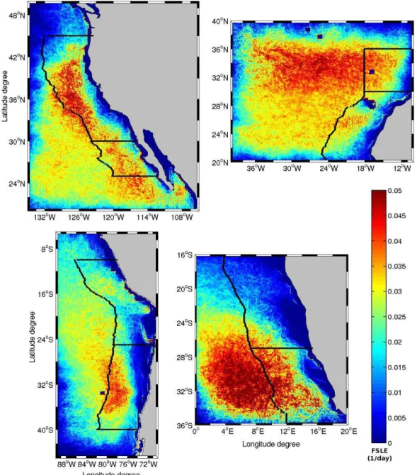
In Fig. 1 we draw the time average (covering the period June 2000–June 2005) of the FSLEs computed for the four EBUS. For all areas, two different subsystems, according to their mean mixing activity, can be defined. The zonal limits are as follows: 30◦N for the Canary (CUS) and the
Califor-nia upwelling system (CalUS), 27◦S for the Benguela (BUS)
and 25◦S for the Humboldt (HUS). Comparing these four
Fig. 1. Time average over the period June 2000–June 2005 of the FSLEs for the CalUS (upper left), the CUS (upper right), the HUS (lower left), and the BUS (lower right). Black lines indicate the analysis area as 8 degrees coastally oriented strips and the corresponding subdivisions.
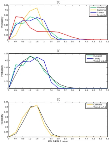
To further quantify the variations in the stirring we exam-ine the probability density functions (PDF) of FSLEs. These distributions are calculated for the FSLEs’ time average nor-malized by the mean values from all grid points within each area (Fig. 2a). For all regions except the BUS (red line), the PDFs have a similar shape: their distributions are broad and slightly asymmetric, with a peak at low mixing activity and a quite long tail of high mixing. However the width and peak values vary depending on the considered system. The PDF of the BUS exhibits a particular asymmetric shape: we can
the CalUS exhibits a thinner and higher peak as compared to the others, indicating that the mean mixing is moderate and quite homogeneous over the entire analysis area (high occurrence of values close to 1, meaning many values are found around the spatial mean). Waugh and Abraham (2008) showed that the PDFs of FTLEs (for Finite-Time Lyapunov Exponents) have a near-universal distribution in the global open surface ocean since they are reasonably well fit by Weibull distributions following: P (λ)=b
a λ a
b−1
exp(−λb
ab ),
witha=λ/0.9 and b=1.6−2.0. We expected a similar be-havior for FSLEs because of the close relation among these quantities. We confirmed that normalized PDFs computed over the upwelling areas are quite well fitted by a Weibull distribution with parameters close to those proposed by these authors, except for the BUS. In Fig. 2b, the normalized PDFs of FSLEs from the CUS and HUS are quite well modeled by a Weibull distribution with parameterb=2.2 whereas the PDFs’ from CalUS (Fig. 2c) fits better a Weibull distribu-tion with parameterb=3.4 related with the higher and thinner peak around the average. The particular shape of the PDF of normalized FSLEs over the BUS indicates again that mixing in this upwelling system is much more heterogeneous. 4.1.2 Temporal evolution of the mixing intensity along
the period 2000–2005
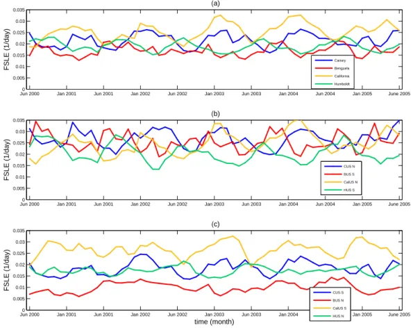
A more detailed comparison between the different subsys-tems can be performed by calculating the time evolution of the spatial averages over the analysis area of each of the four upwellings (Fig. 3a) and each subsystem (Fig. 3b and c). First of all we can sort each area according to their global averaged mixing activity. The mixing in the CalUS appears to be the most vigorous one (spatial average over the whole period: 0.025 day−1), followed by the CUS (0.021 day−1), and finally the HUS (0.019 day−1) and BUS (0.017 day−1) which presents the lowest mixing activity. A strong annual signal is observed in the time evolution of the mixing in the Humboldt, Canary and California upwelling systems. The five peaks of high mixing, corresponding to the five years of data, reflect the seasonal variability of the surface wind. In each hemispheric winter, the sea surface exhibits a more turbulent behaviour due to stronger winds. The last year of these time series reveals a somewhat different pattern of mix-ing, with a double peak for both upwellings of the North-ern Hemisphere, suggesting that 2005 might be a particu-lar year. In fact, this event has been already documented by Schwing et al. (2006) who studied the large-scale atmo-spheric forcing that contributed to these unusual physical oceanic conditions and the associated ecosystems responses. Note that both systems of the Northern Hemisphere oscil-late in phase and are out of phase with the Southern Hemi-sphere systems. Periods of minimum turbulence values, for instance in the HUS, occur from March through May and co-incide with the upwelling relaxation period, linked with the coastal wind regimes. A similar observation may be done for
0 0.4 0.8 1.2 1.6 2 2.4 2.8 3.2 3.6 4 4.4 4.8 5.2 5.6 0
0.05 0.1 0.15 0.2 0.25 0.3 0.35
Probability
(a)
Humboldt California Canary Benguela
0 0.4 0.8 1.2 1.6 2 2.4 2.8 3.2 3.6 4 4.4 4.8 5.2 5.6 0
0.05 0.1 0.15 0.2 0.25
Probability
(b)
Humboldt Canary Weibull b=2.2
0 0.4 0.8 1.2 1.6 2 2.4 2.8 3.2 3.6 4 4.4 4.8 5.2 5.6 0
0.05 0.1 0.15 0.2 0.25 0.3 0.35
Probability
FSLE/FSLE mean
(c)
California Weibull b=3.4
Fig. 2. (a) Normalized Probability Density Function calculated over the FLSEs time average of Fig. 1 for each EBUS (whole analysis area, i.e. 8 degrees coastal strip). Panels (b) and (c) same as in (a) for three of the PDFs fitting a Weibull distribution.
Jun 20000 Jan 2001 Jun 2001 Jan 2002 Jun 2002 Jan 2003 Jun 2003 Jan 2004 Jun 2004 Jan 2005 June 2005 0.005
0.01 0.015 0.02 0.025 0.03 0.035
FSLE (1/day)
(a)
Canary Benguela
California Humboldt
Jun 2000 Jan 2001 Jun 2001 Jan 2002 Jun 2002 Jan 2003 Jun 2003 Jan 2004 Jun 2004 Jan 2005 June 2005 0
0.005 0.01 0.015 0.02 0.025 0.03 0.035
FSLE (1/day)
(b)
CUS N BUS S
CalUS N HUS S
Jun 2000 Jan 2001 Jun 2001 Jan 2002 Jun 2002 Jan 2003 Jun 2003 Jan 2004 Jun 2004 Jan 2005 June 2005 0
0.005 0.01 0.015 0.02 0.025 0.03 0.035
time (month)
FSLE (1/day)
(c)
CUS S BUS N CalUS S
HUS N
Fig. 3. (a) Spatial average versus time of the backward FSLEs. Spatial averages are computed over the analysis areas (8 degrees coastal strip): Canary (blue), Benguela (red), California (yellow) and Humboldt (green); (b) Same as in (a) but for the most temperate subsystems; (c) Same as in (a) but for the tropical subsystems.
it might be the most turbulent one. However the picture is more complex due to the particular temporal evolution of their mixing activity. Initially slightly less active than the southern one, the northern subsystem exhibits a positive ten-dency of increase, whereas the former is characterized by a flat long term pattern. As a consequence, the temperate subsystem becomes more turbulent than the tropical one at around year 2003. These different behaviors of the north-ern and southnorth-ern CalUS subsystems were recently studied by Bograd et al. (2009) using newly developed upwelling in-dex. Finally, the CalUS is quite particular as compared to the others since its horizontal mixing activity is more homoge-neous: when averaging it over space and time in each sub-system, the FSLE means are very comparable, the southern one being slightly higher. Comparing these four upwelling zones, one can note that in the most turbulent temperate sub-systems the values of the FSLEs are quite similar: within the range 0.018–0.04 day−1, i.e., horizontal mixing times be-tween 40 and 90 days. On the contrary, the least active trop-ical subsystems (excluding Southern California) are charac-terized by FSLE ranges from 0.003–0.025 day−1equivalent
to horizontal mixing times from 65 to 530 days. Again on Fig. 3b and c, the mixing activity of the four subsystems from the Northern Hemisphere seems to vary in phase and shows a minimum during the boreal summer/autumn. On the other hand, in the BUS and HUS, the most turbulent tem-perate systems exhibit a visible annual cycle, with a mini-mum occurring during the austral summer/autumn, whereas the least active tropical ones show a high non linear variabil-ity and no obvious trend. Note that the northern BUS shows the smallest mixing activity of all areas.
The high spatio-temporal variability of the surface mix-ing revealed from FSLEs may strongly modulate the biolog-ical components of these complex and dynamic ecosystems. Next we proceed to investigate the correlation between hor-izontal mixing with the biological activity in our regions of interest.
4.2 Relationship with the biological activity
0 0.01 0.02 0.03 0.04 0
0.2 0.4 0.6 0.8 1 1.2
FSLE (1/day)
Mean Chloro (mg/m3)
(a)
Canary Benguela
California Humboldt
0 0.01 0.02 0.03 0.04 0
0.2 0.4 0.6 0.8 1 1.2
FSLE (1/day)
(b)
Canary S Canary N
Benguela S Benguela N
California S California N
Humboldt S Humboldt N
−1 0 1 2 3
0 0.2 0.4 0.6 0.8 1 1.2
(c)
Westward Ekman Transport (m2/s)
0 0.01 0.02 0.03 0.04
0 0.5 1 1.5 2 2.5
FSLE (1/day)
Mean Chloro (mg/m3)
(d)
Canary Benguela
California Humboldt
0 0.01 0.02 0.03 0.04
0 0.5 1 1.5 2 2.5
FSLE (1/day)
(e)
Canary Benguela
California Humboldt
0 0.01 0.02 0.03 0.04
0 0.5 1 1.5 2 2.5
FSLE (1/day)
(f)
Canary Benguela
California Humboldt
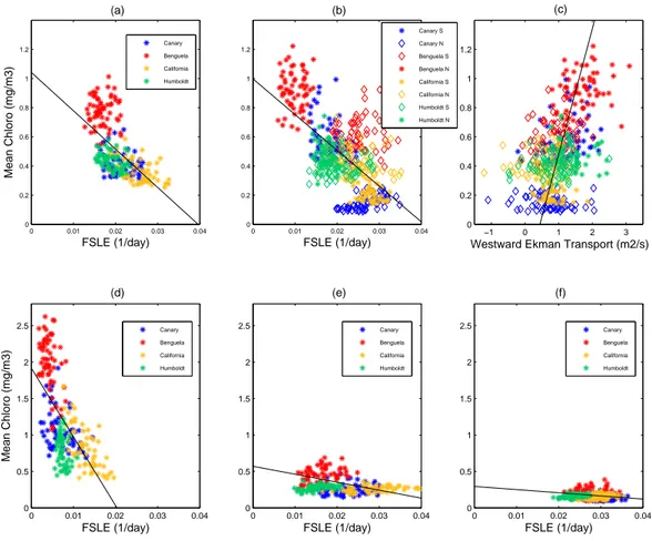
Fig. 4. Chlorophyll-aversus backward FSLEs, both averaged over the analysis areas (8 degrees coastal strips) for: (a) Whole analysis areas (R2=0.38); (b) Same as in (a) but per subsystem (R2=0.43); (c) Same as in (b) but for chlorophyll-aversus westward Ekman transport per subsystem (R2=0.21; for visual improvement, the regression line has been obtained with the opposite order, x-axis versus y-axis); (d, e, f) Same as in (a) but for three successive strips oriented along the coast, (d) 2◦from the coast, (e) within the 2◦to 5◦coastally oriented strip and (f) within the 5◦to 9◦coastally oriented strip.
distribution in the four upwellings by averaging the chloro-phyll concentration along lines of constant latitude within the analysis areas for our five years of study (not shown). In each upwelling system, a clear distinction appears between two different zones, a southern one and a northern one, char-acterized by a very distinct degree of chlorophyll richness. In fact, the limits of the subsystems observed in the chloro-phyll concentration Hovm¨oller plots coincide with the previ-ous latitutinal limits deduced from FSLEs (around 30◦N for
CUS and CalUS, 27◦S for BUS and 25◦S for HUS). We also
noticed that the poorest subsystem in chlorophyll matches the most turbulent one and vice-versa; this remark stands for the four EBUS. The spatial averaged chlorophyll over each analysis area (8◦degrees coastal strips) reveals that the
BUS admits the highest chlorophyll-acontent (0.78 mg/m3), followed by the HUS (0.43 mg/m3), CUS (0.42 mg/m3) and CalUS (0.36 mg/m3). This ranking is just the opposite as the one based on the mixing activity of the surface ocean.
calculations of spatial means over strips oriented along the coast (see Fig. 4, three lower panels d, e, and f), we observe a high negative correlation at the coast, decreasing when shift-ing to offshore strips, and even becomshift-ing flat when approach-ing the oligotrophic gyre further offshore. This findapproach-ing ob-tained from an analysis over the four EBUS seems to indicate a variable response of the biology to physical stirring, valid in such diverse areas widespread over the world ocean.
Upwelling areas are definitely affected by water vertical movements and velocities, through uplift of rich nutrients water and 3-D turbulence, which are not captured by our previous analysis. We will also examine the influence of Ek-man transport which creates pumping of nutrients and carries them from the deep layer to the coastal surface waters where light is not limiting. Vertical velocities and Ekman transport, which can both play a very relevant role in the chlorophyll signature detected from space, will be considered in the fol-lowing.
We evaluated the horizontal divergence,1, of the surface velocity field and averaged it over the period June 2000– June 2005 at each point of the CUS, BUS, CalUS and HUS (not shown). The negative values of the 1 field in the coastal areas indicates the presence of upwelling events. We noticed that in the coastal zones of the BUS, the well known upwelling cells Cape Frio, Walvis Bay and L¨uderitz in the northern subsystem appear clearly, being more intense than the southern cells, in agreement with Monteiro (2009) estimates of the northern subsystem ac-counting for 80%, on average, of the total upwelled flux over the whole BUS. The intense upwelling cells spread along the Peru/Chile coast are also visible, whereas the area above 15◦S is mainly characterized by negative velocities
which represent the equatorial upwelling. When averaging the temporal mean of the1field over the analysis area of each subsystem, representing a measure of the mean ver-tical velocities averaged over space and time, we confirm that the less (most) horizontally stirred system is associ-ated with negative (positive) mean vertical velocities indicat-ing predominance of upwellindicat-ing phenomena (downwellindicat-ing, respectively). This stands for the BUS, HUS and CUS since their less turbulent systems are respectively character-ized by1nBUS=−0.0036 day−1,1nHUS=−0.002 day−1and
1sCUS=−0.0016 day−1whereas their most turbulent exhibit positive means (1sBUS=0.0012, 1sHUS=2.2×10⁻⁴day−1 and1nCUS=8.7×10⁻⁴day−1). For the CalUS, the distinc-tion of two different subregions is not so clear, as compared to the others, confirmed by the very close negative average
1nCalUS=−8×10⁻⁴day−1 and 1sCalUS=−1×10⁻³day−1. It seems that areas dominated with upward processes are re-stricted to the very coastal areas whereas the offshore waters are dominated by downward ones. The global averages of
1over the whole domain reveal negative values (upwelling) and give the following ranking: the most intense upward ve-locities are found in the BUS, followed by the CalUS, then comes the HUS and finally the CUS.
To complete the analysis, we have calculated the Ekman transportUE along the E-W direction. Not surprisingly, its
spatial distribution (not shown) is particularly linked to the spatial distribution of chlorophyll: high chlorophyll contents are often associated with intense Ekman transport, indicat-ing high upwellindicat-ing intensity. Indeed the northern regions of the BUS and HUS, the richest in chlorophyll and present-ing the minimum mixpresent-ing activity, are characterized by the highest offshore transport. In the CUS, both sub-areas have high values for the offshore transport very close to the coast, with similar values in the southern and northern subregions. Further from the coast, the highest westward transport in the southern CUS area coincides again with the highest chloro-phyll content. The same analysis may be done for the CalUS with a less marked difference in the offshore southern sub-system. Figure 4c represents the spatially averaged west-ward Ekman transportUEversus spatial averages of
chloro-phyll concentration, over each subsystem from June 2000 to June 2005 (one point per month). Negative values indicate an Ekman transport to the east, whereas positive ones in-dicate an offshore Ekman transport to the west. A positive correlation appears confirming the effect of Ekman-transport induced upwelling on biological productivity. This finding is not surprising and compatible with previous results (Thomas et al., 2004) since horizontal currents are strongly related to the vertical circulation. A global average of Ekman transport over space (analysis areas) and time reveals similar ranking deduced from the chlorophyll content, except a shift between CUS and HUS. The BUS has the highest (−1.33 m2/s), then come the CUS (−1.07 m2/s) and HUS (−1.01 m2/s) and fi-nally the CalUS (−0.7 m2/s).
5 General discussion
Weibull distribution, with slightly different parameters val-ues as indicated in Waugh and Abraham (2008), they can be considered as large-strain regions. The PDF of normalized FSLEs over the BUS shows a particular distribution, indicat-ing that the mixindicat-ing activity over this system is quite unique. The ranking in terms of chlorophyll content is the same than the one proposed by Cushing (1969), linking chlorophyll content and higher trophic level production. Carr (2001) and Carr and Kearns (2003) compared the EBUS depending on their primary productivity estimated from remote sensing and found also the same ranking, except for a switch between the HUS and CUS. The temporal variations of the chloro-phyll stocks and their coupling with Ekman transport was studied in details by Thomas et al. (2004) over the four EBUS and more precisely over the CUS by Lathuili`ere et al. (2008). We globally confirmed that chlorophyll stocks are positively correlated with westward Ekman transport intensity.
When investigating the link of FLSEs with biological data, the scatterplots reveal a negative correlation between hori-zontal mixing activity and chlorophyll concentration in up-welling areas. This negative effect is in line with Lachkar et al. (2009) who showed that strong eddy activity acts as an inhibiting factor for the biological productivity in coastal up-welling systems. They confirmed that the CUS and CalUS appear to be the most contrasting systems of the 4 EBUS, in terms of biological productivity and mixing activity as well. Patti et al. (2008) also mentioned a negative correlation be-tween turbulence, calculated as the cube of wind speed, and logarithm of the chlorophyll-a concentration for the BUS; however this finding did not hold for the other areas show-ing a positive relationship. We note that theoretical stud-ies in idealized settings, in which nutrients reach plankton only by lateral stirring, display also negative correlation be-tween mixing and biomass (although mixing and productiv-ity may be positively correlated) (T´el et al., 2005; Birch et al., 2007; McKiver and Neufeld, 2009). In the following we propose some mechanisms to explain this inverse relation-ship, as compared to the open ocean and other low nutrient environments, where several studies showed that eddies and turbulent mesoscale features tend to rather enhance biolog-ical productivity (McGillicuddy et al., 1998; Oschlies and Garc¸on, 1998).
In our case, we focussed on very productive areas where the high biological productivity is maintained by a large nu-trient supply from deep waters driven by Ekman pumping. Horizontal turbulent mixing of nutrients in surface waters, which was significant in the oligotrophic areas, is now a sec-ond order effect as compared to the vertical mechanisms (nu-trient Ekman pumping) in the most productive subsystems. McKiver and Neufeld (2009), lay the emphasis on a ratio between the biological ecosystem timescale (inverse of the growth rate) and the flow timescales. When increasing the ratio, corresponding to an increase of turbulence, they indi-cate a negative effect on the phytoplankton mean concentra-tion as it is the case in our study. The localized pulses of
nu-trients are rapidly being dispersed by intense mixing before being used efficiently by the phytoplankton to grow. Similar processes were documented in a theoretical modeling study from Pasquero et al. (2005). When associating an upwelling of nutrient with coherent vortices, they find a lower primary productivity than without vortices. They explained this ob-servation by the trapping properties of eddies and the lim-ited water exchange between the vortex cores and the sur-rounding waters. Eddies are able to trap and export offshore rich coastal waters which are not being used efficiently by the phytoplankton, resulting in a lateral loss of nutrients of the coastal upwelling. We also observed that areas charac-terized by high FSLEs are correlated with intense vertical movements (downwellings as well as upwellings), whereas the areas with low FSLEs are mainly dominated by upward vertical velocities (upwellings). Lehahn et al. (2007) recently showed that vertical motions associated with eddy are more precisely located close to the lines of high FSLEs. Regions of high FSLE averages indicate a high occurrence of intense eddies which modify the three dimensional mean flow. The nutrient Ekman pumping, dominant process in upwelling ar-eas, is weakened and the fuelling of nutrients toward the sur-face decreased. A significant stirring revealed by high FSLEs may decrease the Ekman transport induced upwelling lead-ing to weaker surface chlorophyll stocks.
In the scope of previous works concentrating in the open ocean, and considering Fig. 4 (3 lower panels), we suggest the possibility of a variable response of the phytoplankton to the mesoscale oceanic turbulence. This changing behav-ior, represented by the high negative correlation at the coast decreasing when moving offshore, may be explained when considering the different dominant processes in the areas of interest. In very coastal areas, intense biological productiv-ity is supported by the intensproductiv-ity of Ekman induced upwelling of nutrients. However, a high turbulence caused by eddies may induce an offshore lateral loss of nutrients and may de-crease the vertical fuelling of surface waters from nutrients Ekman pumping, thus leading to a negative effect on biolog-ical production. Then, when moving offshore in the transi-tional area between the very coastal upwelling and the olig-otrophic gyre, the moderate production regime relies on the offshore export of coastal rich waters. In this case, the tur-bulent mixing of nutrients may have a minor influence on moderate productivity, from the compensation of weak posi-tive and negaposi-tive effects. Then, in the open ocean where the biological productivity is weak and limited by very low nutri-ent concnutri-entrations, the resultant effect of horizontal mixing on phytoplankton growth becomes positive. The phytoplank-ton development is being promoted by eddies which induce vertical velocities and an upward flux of nutrients toward the very depleted surface waters (McGillicuddy et al., 1998; Os-chlies and Garc¸on, 1998).
iden-tify the main factors among the four EBUS. Carr and Kearns (2003) distinguished different types of factors and discussed which ones control primary productivity. Oxygen concen-trations and displacement of the thermocline symbolized the large-scale upwelling intensity; the local forcings were rep-resented by quantities such as Photosynthetically Available Radiation, offshore transport and SST gradient, but the au-thors omitted the turbulence. They showed that large-scale circulation patterns are responsible for the main differences between EBUS. Then, the local forcings, and their combina-tion with large-scale factors, explain the weaker variacombina-tions. If we would consider only the nutrient concentration and Ek-man pumping intensity (from their study) on one hand, and the turbulence from FSLEs (from our study) on the other hand, we can easily explain differences among EBUS with-out taking into account all other factors. Here we argue that adding our turbulence data from FSLEs to nutrients concen-tration and Ekman transport intensity allow us to simply ob-tain similar results, suggesting the fact that the turbulence effect is important to be considered. Patti et al. (2008) stud-ied the factors driving the chlorophyll content and they found that nutrient local concentrations, mainly governed by local upwelling intensity (Ekman pumping), explain the main dif-ferences between very productive areas (HUS and BUS) as compared to the other two (CalUS and CUS). These pro-cesses act as first order factors whereas the continental shelf width appears to be the key secondary order factor explain-ing the difference between HUS and BUS, also mentioned by Carr and Kearns (2003). The mixing from FSLEs can also explain the main differences observed since the CalUS and CUS admit the highest surface mixing activity. More-over, the highest chlorophyll content observed in the northern Benguela coincides again with the minimum of mixing mea-sured by FSLEs. The BUS appears to be the most productive system since the Ekman pumping over a large width shelf is maximum and associated with the lowest mixing. Patti et al. (2008) also discussed other factors such as light limitation, solar cycle, presence of retention areas, etc., concluding that they should act at different levels, in different areas. It is also well known that micronutrient availability and alterna-tive biogeochemical processes such as N2fixation or denitri-fication may also play a role in nature. However, the vari-ability among all these factors over all areas is too large to identify trivial patterns. Consequently we did not consider these controls as primary factors in our analysis.
6 Conclusions
The distribution of FLSEs computed from multi-sensor ve-locity fields over a 5 year period allowed us to make a comparative study of the mixing activity in the four east-ern boundary upwelling systems. Each area was divided into two subsystems showing different levels of temporal aver-aged horizontal stirring rates. When studying the temporal
evolution of their spatially averaged mixing, we proposed a ranking in terms of horizontal mixing intensity for all four EBUS. We also found that the more vigorous mixing oc-curs in subsystems further away the equator explained by the intensification of large scale atmospheric forcing at higher latitudes. Systems from the same hemisphere seem to ex-hibit a similar behavior with a dominant annual cycle. The PDF computations of FSLEs reveal the statistical structure of these Lagrangian diagnostics. When investigating the link of FSLEs with biological data, the subdivisions detected from FSLEs’ maps appeared to be also visible on chlorophyll con-centration Hovm¨ollers suggesting that these two quantities are linked. The scatterplots revealed a negative correlation between horizontal mixing activity and chlorophyll concen-tration in upwelling areas. We then confirmed that chloro-phyll stocks are positively correlated with westward Ekman transport intensity over the four EBUS. It thus seemed that the horizontal turbulent mixing of nutrient is a second order effect as compared to the vertical mechanisms. After esti-mating the mean vertical velocities from incompressibility assumption, we proposed another explanation: the regions of high FSLEs are characterized by occurence of intense eddies and their verticals velocities associated. This will modify the whole 3-D flow and lead to a global decrease of the nutrient Ekman pumping (supported by low Ekman transport). We finally suggest the possibility of a variable response of the phytoplankton to the sub/mesoscale oceanic turbulence de-pending on the distance to the coast. This changing behavior is represented by the high negative correlation at the coast de-creasing when moving offshore. It may be explained when considering the different areas and their associated dominant bio-physical processes. We then discuss the effect of others factors not considered here, and compare our approach to all previous comparative works.
Further work should investigate the robustness of the rela-tionship found in our four systems when examining FSLEs versus biological stocks. Still much needs to be done to fully understand how plankton distributions are controlled by the interplay between their turbulent medium and the non-linear processes of their ecology. Coupled modelling approaches appear to be the only way to consider all these factors si-multaneously. Besides a better understanding of the interac-tions between biological and physical processes, these cou-pled modelling studies will allow us to investigate and deter-mine the respective effect of abiotic and biotic factors.
interface will gain in accuracy when considering this effect through, for instance, a spatial parameterization of turbu-lence.
Acknowledgements. V. R. and C. L. were awarded a
EUR-OCEANS network of Excellence short visit grants. V. R. is supported by a PhD grant from Direction G´en´erale de l’Armement. V. G. and J. S. acknowledge funding support from CNES and C. L. and E. H.-G. from PIF project OCEANTECH of the Spanish CSIC and FISICOS (FIS2007-60327) of MEC and FEDER. We also thank A.M. Tarquis and the two anonymous referees for their constructive comments.
Edited by: A. Turiel
Reviewed by: A. M. Tarquis and two other anonymous referees
The publication of this article is financed by CNRS-INSU.
References
Artale, V., Boffetta, G., Celani, A., Cencini, M., and Vulpiani, A.: Dispersion of passive tracers in closed basins: Beyond the diffu-sion coefficient, Phys. Fluids, 9, 3162–3171, 1997.
Aurell, E., Boffetta, G., Crisanti, A., Paladin, G., and Vulpiani, A.: Predictability in the large: an extension of the concept of Lya-punov exponent, J. Phys. A, 30, 1–26, 1997.
Beron-Vera, F. J., Olascoaga, M. J., and Goni, G. J.: Oceanic mesoscale eddies as revealed by Lagrangian coherent structures. Geophys. Res. Lett., 35, L12603, doi:10.1029/2008GL033957, 2008.
Birch, D. A., Tsand, Y. K., and Young, W. R.: Bounding biomass in the Fisher equation, Phys. Rev. E, 75, 066304, 2007.
Boffetta, G., Lacorata, G., Redaelli, G., and Vulpiani, A.: Detecting barriers to transport: A review of different techniques, Phys. D, 159, 58–70, 2001.
Bograd, S. J., Schroeder, I., Sarkar, N., Qiu, X., Sydeman, W. J., and Schwing, F. B.: Phenology of coastal upwelling in the California Current, Geophys. Res. Lett., 36, L01602, doi:10.1029/2008GL035933, 2009.
Carr, M. E.: Estimation of potential productivity in Eastern Bound-ary Currents using remote sensing, Deep-Sea Res. II, 49, 59–80, 2001.
Carr, M. E. and Kearns, E. J.: Production regimes in four Eastern Boundary Current Systems, Deep-Sea Res. II, 50, 3199–3221, 2003.
Chavez, F. P. and Toggweiler, J. R.: Physical estimates of global new production: The upwelling contribution, in: Upwelling in the Ocean: Modern Processes and Ancient Records, John Wiley and Sons Ltd., 313–320, 1995.
Cushing, D. H.: Upwelling and fish production, in FAO Fisheries Technical Papers, 84, 1–40, 1969.
d’Ovidio, F., Fern´andez, V., Hern´andez-Garc´ıa, E., and L´opez, C.: Mixing structures in the Mediterranean Sea from finite-size Lyapunov exponents, Geophys. Res. Lett., 31, L17203, doi:10.1029/2004GL020328, 2004.
d’Ovidio, F., Isern-Fontanet, J., L´opez, C., Hern´andez-Garc´ıa, E. and Garc´ıa-Ladona, E.: Comparison between Eulerian diagnos-tics and Finite-Size Lyapunov Exponents computed from Altime-try in the Algerian basin, Deep-Sea Res. I, 56, 15–31, 2009. Haller, G.: Lagrangian structures and the rate of strain in a
parti-tion of two dimensional turbulence, Phys. Fluids, 13, 3365–3385, 2001.
Kang, J., Kim, W., Chang, K., and Noh, J.: Distribution of plank-ton related to the mesoscale physical structure within the sur-face mixed layer in the southwestern East Sea, Korea, J. Plankton Res., 26(12), 1515–1528, 2004.
Koh, T. and Legras, B.: Hyperbolic lines and the stratospheric polar vortex, Chaos, 12, 382–394, 2002.
Lachkar, Z., Gruber, N., and Plattner, G. K.: A comparative study of biological productivity in Eastern Boundary Upwelling Systems using an Artificial Neural Network, Biogeosciences Discus., sub-mitted, 2009.
Lathuili`ere, C., Echevin, V., and L´evy, M.: Seasonal and intraseasonal surface chlorophyll-a variability along the northwest African coast, J. Geophys. Res., 113, C05007, doi:10.1029/2007JC004433, 2008.
Lehahn, Y., d’Ovidio, F., L´evy, M., and Heyfetz, E.: Stirring of the Northeast Atlantic spring bloom: a Lagrangian analy-sis based on multisatellite data, J. Geophys. Res., 112, C08005, doi:10.1029/2006JC003927, 2007.
Mackas, D., Tsurumi, M., Galbraith, M., and Yelland, D.: Zoo-plankton distribution and dynamics in a North Pacific Eddy of coastal origin: II. Mechanisms of eddy colonization by and re-tention of offshore species, Deep-Sea Res. II, 52, 1011–1035, 2005.
Mackas, D., Strub, P. T., Thomas, A. C., and Montecino, V.: Eastern Ocean Boundaries Pan-Regional View, in: The Sea, Chapter 2, p 21–60, edited by: Robinson, A. R. and Brink, K. H., Harvard Press Ltd., 2006.
McGillicuddy J., Robinson A., Siegel D., Jannasch H., Johnson R., Dickey T., McNeil, J., Michaels, A., and Knap, A.: Influence of mesoscale eddies on new production in the Sargasso Sea, Nature, 394, 263–266, 1998.
McKiver, W. J. and Neufeld, Z.: The influence of turbulent advec-tion on a phytoplankton ecosystem with non-uniform carrying capacity, Phys. Rev. E., 79, 061902, 2009.
Monteiro, P. M. S.: Carbon fluxes in the Benguela Upwelling sys-tem, in: Carbon and Nutrient Fluxes in Continental Margins: a Global Synthesis, chapter 2.4, edited by: Liu, K. K., Atkinson, L., Qui˜nones, R. and Talaue-McManus, L., to appear (October), 2009.
Moore, T., Matear, R., Marra, J., and Clementson, L.: Phytoplank-ton variability off the Western Australian Coast: Mesoscale ed-dies and their role in cross-shelf exchange, Deep-Sea Res. II, 54, 943–960, 2007.
Olascoaga, M. J., Beron-Vera, F. J., Brand, L. E., and Kocak, H.: Tracing the early development of harmful algal blooms with the aid of Lagrangian coherent structure, J. Geophys. Res., 113, C12014, doi:10.1029/2007JC004533, 2008.
pri-mary production in a model of the North Atlantic Ocean, Nature, 394, 266–268, 1998.
Owen, R. W.: Fronts and Eddies in the sea: mechanisms, interac-tions and biological Effects, in: Fronts and Eddies in the Sea, p 197–233, edited by: Owen, R.W., Academic Press, London, 1981.
Patti, B., Guisande, C., Vergara, A.R., Riveiro, I., Barreiro, A., Bo-nanno, A., Buscaino, A., Basilone, G., and Mazzola, S.: Fac-tors responsible for the differences in satellite-based chlorophyll
aconcentration between the major upwelling areas, Est. Coast. Shelf Sc., 76, 775–786, 2008.
Pasquero, C., Bracco, A., and Provenzale, A.: Impact of the spatiotemporal variability of the nutrient flux on primary productivity in the ocean, J. Geophys. Res., 110, C07005, doi:10.1029/2004JC002738, 2005.
Pauly, D. and Christensen, V.: Primary production required to sus-tain global fisheries, Nature, 374, 255–257, 1995.
Rio, M.-H. and Hern´andez F.: A mean dynamic topography com-puted over the world ocean from altimetry, in-situ measure-ments, and a geoid model, J. Geophys. Res., 109, C12032, doi:10.1029/2003JC002226, 2004.
Rossi, V., L´opez, C., Sudre, J., Hern´andez-Garc´ıa, E., and Garc¸on, V.: Comparative study of mixing and biological activity of the Benguela and Canary upwelling systems, Geophys. Res. Lett., 35, L11602, doi:10.1029/2008GL033610, 2008.
Ryther, J. H.: Photosynthesis and fish production in the sea, Sci-ence, 166, 72–76, 1969.
Schwing, F. B., Bond, N. A., Bograd, S. J., Mitchell, T., Alexander, M. A., and Mantua, N.: Delayed coastal upwelling along the U.S. West Coast in 2005: A historical perspective, Geophys. Res. Lett., 33, L22S01, doi:10.1029/2006GL026911, 2006.
Shadden, S. C., Lekien, F., and Marsden, J. E.: Definition and prop-erties of Lagrangian coherent structures from finite-time Lya-punov exponents in two-dimensional aperiodic flows, Phys. D, 212, 3–4, 271–304, 2005.
Sudre, J. and Morrow, R.: Global surface currents: a high resolution product for investigating ocean dynamics, Ocean Dyn., 58(2), 101–118, 2008.
T´el, T., de Moura, A., Grebogi, C., and Karolyi, G.: Chemical and biological activity in open flows: A dynamical system approach, Phys. Rep., 413, 91–196, 2005.
Thomas, C. A., Strub, T. P., Carr, M. E., and Weatherbee, R.: Com-parisons of chlorophyll variability between the four major global eastern boundary currents, Int. J. Rem. Sens., 25, 7, 1443–1447, 2004.