Abstract
Niobium metallurgical recovery measures how much of the metal content in the ore is separated in the concentrate after the mineral processing stages. This information can be obtained through laboratory tests with ore samples obtained during drilling. Thereunto, representative ore samples are subjected to tests mimicking the ore concen-tration processing low, but these experiments are time consuming and costly.
The main objective of this study was to develop a more eficient way to obtain the metallurgical recovery information from ore samples. Based on the development of chemometrical studies, the chemical components currently analyzed in the ore with correlation to the metallurgical recovery were identiied. These correlated variables were used to build a nonlinear multivariate regression model to explain the response variable, i.e. metallurgical recovery.
The Principal Component Analysis was used in this work to deine which chemical variables contribute most to explain the metallurgical recovery phenomenon. The Sec-ond order regression equation (Response Surface) was the most suitable methodology to explain the metallurgical niobium recovery and was created by the interaction of the ive most important chemical variables.
After the exclusion of outliers, the linear regression coeficient between the metal-lurgical recovery calculated and the metalmetal-lurgical recovery analyzed was 82.59%.
The use of the second order regression equation contributes to reduce the amount of experimental analysis to assess the geometallurgical niobium ore response, promot-ing the reduction of costs for metallurgical characterization of the ore samples. The methodology proposed proved to be eficient, maintaining an adequate precision in the forecasted response.
Keywords: chemometrics, mining industry; Response Surface; geometallurgy; multi-variate statistics.
Jose Marques Braga Junior
Mestrando
Universidade Federal do Rio Grande do Sul – UFRS Departamento de Engenharia de Minas Porto Alegre - Rio Grande do Sul – Brasil [email protected]
Engenheiro-Geólogo da Companhia Brasileira de Metalurgia e Mineração - CBMM - Homogeneização Araxá - Minas Gerais – Brasil
João Felipe Coimbra Leite Costa
Professor Titular
Universidade Federal do Rio Grande do Sul – UFRS Departamento de Engenharia de Minas - PPGEM-DEMIN Porto Alegre - Rio Grande do Sul – Brasil
Applying chemometrics to
predict metallurgical niobium
recovery in weathered ore
Mining
Mineração
http://dx.doi.org/10.1590/0370-44672016710097
1. Introduction
During the development of a min-ing project, in which there is mineral or metal processing to concentrate the metal of interest, it is important to know the geometallurgical response from the ore at the plant, as this is the main fac-tor affecting mineral chain proitability. This information helps to maximize the economic beneit of the project through the integration of geological knowledge, mining, mineral processing, environmen-tal controls and the market.
The metallurgical recovery informa-tion can be obtained experimentally at a pilot plant or by lab tests. Thus, represen-tative ore samples are subjected to tests mimicking the ore concentration process-ing low. These experiments demand time
and are costly. One way to reduce the cost of these experiments is to identify chemical components currently analyzed in the ore with possible correlation with the metal-lurgical recovery. These correlated vari-ables can be used to build a multivariate regression model (linear or nonlinear) to explain the response variable, i.e. metal-lurgical recovery.
To build and use models to predict and explain a phenomenon accurately, a careful selection is initially necessary to deine the most signiicant variables that will explain in part, or in whole, the sys-tem’s behavior. Although many variables and parameters is necessary to predict a response variable, a small number of variables, in general, explains much of it.
Thus, the irst stage of a modeling process is to identify the right variables and the relationships among them.
Once the importance of modeling the geometallurgical variable is contex-tualized, it is proposed to investigate the relationships among the variables to explain the ore response at the plant given statistics and additive variables (grades for instance). Therefore, it is necessary to measure the variables that are con-sidered relevant to the understanding of the analyzed phenomenon. Many are the dificulties in converting the information obtained into knowledge, especially when it comes to the statistical evaluation of such information.
106 REM, Int. Eng. J., Ouro Preto, 71(1), 105-110, jan. mar. | 2018
the metallurgical recovery can contrib-ute to reduce the quantity of experimen-tal analyses of this variable, which will directly inluence to reduce costs with the metallurgical characterization of the
ore samples.
In this article, the development of a regression model for calculating the metal-lurgical niobium recovery at various stages of the production process is proposed. The
results of the application are validated against the laboratory test data.
The chemical variables used in the response model are herein referred to as X1, X2, X3, …, X9 for the sake of conidentiality.
2. Material and methods
The data set considered in this study came from a drill hole campaign known as FSA. The samples obtained in this cam-paign were tested in the lab mimicking the processing lowchart and these samples were also chemically analyzed.
Cores from the drill holes were logged and the important geological do-mains were separated into: Soil; Orange weathered ore; Brown weathered ore; Saphrolite and fresh Rock (carbonatite).
Among the ive geological domains mentioned, only one has enough data to be subjected to a multivariate analysis and to provide a meaningful response. This domain is the Orange weathered ore, which is the ore mined at the site.
Principal Component Analysis (PCA) helped in deining which chemi-cal components should be considered in the multivariate regression. This
math-ematical procedure uses an orthogonal transformation to convert a set of ob-servations possibly correlated to a set of linear uncorrelated variables known as principal components. This transforma-tion is deined so that the irst principal component has the greatest variance, and each subsequent component has the maximum variance under the constraint of being orthogonal to the previous components (Pearson, 1901).
The irst stage was the selection of which variables better explain the variance of the response (met recovery). Although many variables and parameters are neces-sary to predict the niobium metallurgical recovery, PCA analysis showed that ive chemical variables (X1, X2, X3, X4 and X5) can explain much of it. So, the other four vari-ables (X6, X7, X8, and X9) were disregarded, as they did not have much to contribute to
explain the plant metallurgical recovery. The second order multivariate regression methodology (Response Surface) was used to calculate the metallurgical recovery based on ive chemical variables. This statistical methodology is commonly used for modeling and analyzing problems in which the dependent variable is inluenced by several factors, and the goal is to opti-mize this response (George, 2007).
The Response Surface may be de-ined as the geometric representation ob-tained when a response variable is plotted as a function of two or more quantitative factors. This function can be deined as:
Y=f ( x1, x2, …, xk)+ε, where Y is the response (dependent variable); and x1, x2, ..., xk are the factors (independent variables); andε is the random error (George, 2007).
In its polynomial equation form, the Response Surface is deined as:
where x1, x2, ..., xk are the independent variables which inluence the response
Y;β0, βi (i = 1, 2, ...,k),βij (j = 1, 2, ...,k) are the unknown parameters; and ε is the random error. (Box and Draper, 1987).
Among the advantages of Response Surface methodology, the main one is that their results are very consistent with
the effects of non-ideal conditions, such as random errors and inluential points, since this methodology is robust. Another advantage is the simplicity of obtaining the polynomials from the analytical Re-sponse Surface methodology. In general, polynomials of two or more variables are continuous functions.
For multivariate regressions and the principal component analysis MINITAB® software was used, which
has a number of statistical tools for both univariate analysis and for multivariate analysis. The software SGeMS was also used to build the maps and the scatter plots (Remy et al., 2009).
3. Results
Among the nine variables consid-ered for the principal component analysis
(X1; X2; X3; X4; X5; X6; X7; X8 and X9), the ones that contributed most to explain the met-allurgical recovery were X1; X2; X3; X4 and
X5, which basically reduced four out of the nine initial number of independent vari-ables. In addition to being able to identify which variables contribute most to explain a given phenomenon using PCA, it is also possible to identify which variables are redundant, which means a very high linear correlation from one variable to another.
The criterion used to make the statement that variables: X1, X2, X3, X4 and
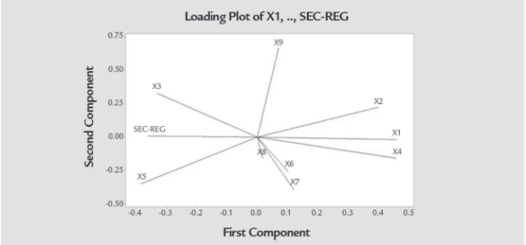
X5 were the most contributed in this study were based on the Loading Plot analyses, which revealed the relationships among
the variables considered in the space of the irst two components. Figure 1 shows the plot of the loadings of the variables on the components. Each variable is a point, whose coordinates are given by the load-ings on the two principal components. In this case the X6, X7 and X8 variables have similar low loadings for the irst component, which is different from the
X9 high loading.
The correlation between a compo-nent and a variable in PCA framework is called loading and it measures the in-formation they share, so factor loadings represent how much a factor explains a variable in factor analysis. It is possible to examine the loading pattern in the Minitab software (Minitab, 2014) factor
loading analysis output to determine the factor that has the largest effect on each variable. Some variables might have high loadings on multiple factors. Factor load-ings can range from -1 to 1. Loadload-ings close to -1 or 1 indicate that the factor strongly affects the variable. Loadings close to zero indicate that the factor has a weak effect on a speciic variable.
The irst component is the most important one. The variables (X1 and
X4) provide more information, and these two variables are also strongly cor-related. The variables X6, X7, and X8 are closely associated and they only provide a small amount of information, as they are close to zero in the irst component. Variable X9 also has a low score in the
Y=
β
0+
∑
kβ
i
x
i+
∑
kβ
ii
x
i2
+
∑
∑
j=2
β
ijx
ix
j+
ε
i=1 i=1k -1 1=1
irst component, and differently from the variables X6, X7, and X8, it has high score in the second component.
According to Abdi and Williams (2010), in general, different meanings of ‘loadings’ lead to equivalent
interpreta-tions of the components. This happens because the different types of loadings dif-fer mostly by their type of normalization.
Figure 1 Factorial load chart considering nine che-mical variables and the metallurgical reco-very analyzed in the laboratory. The first load components are on the x-axis and the second load components on the y-axis.
The squared loadings could be also used to interpret the relationship between the variables. The sum of the squared coeficients of correlation be-tween a variable and all the components is equal to 1. This is due to the fact that the squared loadings give the
propor-tion of the variance of the variables explained by the components.
The irst multiple regression was performed without excluding outlier values. This regression was made in the MINITAB® software, and it was
neces-sary to deine the dependent variable
(DCCG) and the independent variables (X1; X2; X3; X4 and X5) to be used.
Figure 2 shows the result of the irst regression performed without the outlier analysis. Note the scatter plots between the dependent variable and independent ones.
Figure 2 Scatter plots of the first attempt for multi-variable regression. These charts were built considering the independent variables (X1; X2; X3; X4 and X5) and the result of the regression (SEC-REG). The Y-axis represents the values of the calcula-ted metallurgical recovery (SEC-REG) and the X-axis represents the value of the
inde-pendent variables used in the regression
The result of the first regression without residual treatment presented a 65.04% coeficient of determination (R2).
Treating the residual appropriately can lead to a better result, optimizing the dependent variable response without in-luencing the equation representativeness in the geological domain considered.
The residue analysis was irst per-formed excluding the samples that did not contain chemical analysis for any independent variable used for regression (X1; X2; X3; X4 and X5), i.e. keeping only an isotopic subset from the data. Missing data in the chemical analysis of all the variables needed leads to an incorrect
re-sponse model. Then some speciic values that were anomalous to the geological domain considered (Orange weathered ore) were excluded. Some cores were veriied to understand the reasons of the geological anomaly, in most cases, the anomalies are related to veins composed of different minerals cutting the orange weathered ore. In a last stage, a residual analysis was carried out to improve the it (R2) of the proposed data model. No test
was performed to characterize de outliers. During the residual analysis, 202 samples were excluded, corresponding to 13% of the whole data set, where 1406 samples remained in the data set, which
was used to build the regression equation. Using the graph technique (residuals versus itted values), the residuals that had standard deviation exceeding 35% were excluded. After the previous procedure, the linear regression coeficient between the calculated metallurgical recovery and metallurgical recovery analyzed was 82.59%. This correlation between these variables is very high, allowing the use of the regression equation to calculate the metallurgical recovery using the regression with an acceptable error.
The regression equation used to cal-culate the metallurgical recovery, after the residual treatment was deined as:
SEC-REG
= -33,1 - 15,1X
1- 0,09X
2+ 39,08X
3+ 41,91X
4+ 13,53X
5- 2,51X
32- 5,66X
42
-0,62X
52
+2,57X
1X
3108 REM, Int. Eng. J., Ouro Preto, 71(1), 105-110, jan. mar. | 2018
Figure 3
Scatter plot between the analyzed variable (DCCG) and the result of the calculation of the metallurgical recovery using the multi-variate regression equation (SEC-REG).
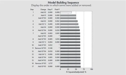
Figure 4 presents the results of the multiple regression obtained with MINITAB® software. It is possible to
see the sequential regression model con-struction with the contribution of each variable, as well as their paired variable
contribution. The variable that contrib-utes most to the model's explanation is
X3, followed by the variable X1, and so on.
Figure 4
Summary of the model building sequence. The sequence is displayed per the contribution level of each
variable or interaction of the variable pairs.
4. Discussion
The application of Response Sur-face methodology has been used in the chemical industry, having its foundations formalized by Box and Draper (1987). In the agronomic ield, it has been used to study the yield, the effect of nutrient levels applied to the soil, including other factors such as planting density and irrigation. Although this method has been very rarely applied in mining, its use has a potential beneit. This methodology is very power-ful and has many applications that can help to easily explain many phenomena involved in the mining industry.
Montgomery (2001) wrote that the Response Surface equations can be
graphi-cally represented and used in three ways as follows:
i. Describing how the test variables affect the answers;
ii. Determining the interrelation-ships between the variables under test; and to
iii. Describe the combined effect of all test variables on the response.
For this speciic work, the target was the use of the combined effects of ive variables (X1, X2, X3, X4 and X5) to explain the metallurgical recovery of niobium.
For the effective use of Response Surface, ive assumptions should be con-sidered (Montgomery, 2001):
i. The factors that are critical to the process must be known;
ii. The region where the factors inlu-ence the process must be known;
iii. The factors must vary continuous-ly along the chosen experimental group;
iv. There is a mathematical function that relates to the factors measured response;
v. The answer that is set by this func-tion is a smooth surface.
Before building the regression model by the Response Surface methodology, it was necessary to perform a careful multivariate statistical data exploratory analysis. The results demonstrate it was possible to apply this methodology to ind Figure 3 shows the scatter plot
between the analyzed variable (DCCG),
obtained from lab tests, and the re-sultant metallurgical recovery using
out the effects of combining the chemical variables in the mineral recovery response during the concentration process.
Per Montgomery (2001), in the ab-sence of suficient knowledge about the true Response Surface, the user usually tries the irst order model. However, when the irst order model is not enough to it the surface, it is necessary to incorporate higher order terms to improve the model itted.
The use of first order regression models, with the same data set used in
this study, showed that the obtained model was insuficient to explain the behavior of metallurgical recovery from the same ive chemical variables. Using this irst order regression model, the best correlation ob-tained was 52% (R2), which has already
been improved after outlier exclusion us-ing residual analysis.
Among all the interactions between the pairs of variables, the interaction be-tween X4 and X3 stands out for the phenom-enon explanation, in addition to the
interac-tion between X3 and X1, and X5and X4 that also exhibit high covariance coeficients.
The quadratic contribution of each variable also helps to deine the regres-sion model. The quadratic contribution of the X4 is more signiicant in this case than the quadratic contribution of X3. The quadratic contribution of other variables are very low.
Figure 5 shows the effect of each independent variable to the response (SEC-REG).
Figure 5 Correlation between the independent va-riables (X1; X2; X3; X4 and X5) and the result
of the regression (SEC-REG). Where the Y-axis represents the values of the calcula-ted metallurgical recovery (SEC-REG) and the X-axis represents the value of the
inde-pendent variables used in the regression
Without the residual analysis, the regression coeficient between the analyzed and calculated metallurgical recovery was 65.04%, which means that the variables con-sidered would explain only 65.04% of the
metallurgical recovery. Even after excluding some outliers that were affecting the regres-sion, there were still 61 high value residues; however, they were kept to avoid creation a false impression of high correlation
exclud-ing data without well-founded criteria. Figure 6 shows the data points with large residual (red dots in the plot) and atypi-cal values of the response variable SEC-REG (blue dots).
Figure 6 Scatter plot between the residuals against the adjusted values.
Figure 7 shows two maps with the drill hole distribution: in the irst map, the colored dots represent the drill holes
with geometallurgical data from labora-tory tests, and the second one, with the calculated geometallurgical data. These
two data can be used together to a build simulation model in order to improve the metallurgical recovery prediction.
Figure 7 Maps showing the drill hole distribution according to the two different
methodolo-gies to obtain the processing results.
110 REM, Int. Eng. J., Ouro Preto, 71(1), 105-110, jan. mar. | 2018
References
Received: 9 September 2016 - Accepted: 25 September 2017.
5. Conclusion
In order to create a model that ex-plains the behavior of the metallurgical recovery, different mathematical regres-sions were tested. Second order multivari-ate regression (Response Surface) proved to be suitable for use in modeling and performance analysis of geometallurgical niobium ore, since the last is inluenced by several factors.
The application of the obtained regression equation was restricted to samples associated with the geological domain “Orange weathered ore”.
Before using the Response Surface methodology, it is important to deine which independent variables contrib-ute to explaining the phenomenon of interest, in this case, the metallurgical recovery of niobium.
The chemical interaction between the independent variables considered, as well as their quadratic interactions, contributed greatly to explain the phenom-enon of niobium metallurgical recovery. Using the multivariate regression equation obtained, it was possible to calculate the
metallurgical recovery for all samples or locations where the chemical variables are known.
The Response Surface method-ology to predict the metallurgical niobium recovery provided processing information, having high correlation with the metallurgical recovery depen-dent data. Using this newly calculated data correctly, it is possible to increase the geometallurgical knowledge and incorporate this information into mine planning.
Acknowledgment
We acknowledge CBMM for allowing using the data and publish these results.
ABDI, H., WILLIAMS, L. J. Principal component analysis. WIREs Computational statistics, New Jersey, v.2, p. 433-459, jun. 2010.
BOX, G. E. P., DRAPER, N. R. Empirical model building and response surface.
New York: John Wiley & Sons, 1987. 688p.
GEORGE, A. L. BOX. Response surface, mixtures, and ridge analyses. (2. Ed.). New Jersey: John Wiley and Sons, 2007. 1-3p.
MINITAB 17. Getting started with Minitab: 17. Minitab, Inc. United States, 2014. 83 p.
MONTGOMERY, D.C. Introduction to statistical quality control. (4. Ed.). New York: John Wiley and Sons, 2001. 816p.
PEARSON, K. On lines and planes of closest it to systems of points in space.
Philosophical Magazine, v. 2, n. 6, p. 559–572, 1901.