www.earth-surf-dynam.net/2/47/2014/ doi:10.5194/esurf-2-47-2014
©Author(s) 2014. CC Attribution 3.0 License.
Earth
Surface
Dynamics
A linear inversion method to infer exhumation rates in
space and time from thermochronometric data
M. Fox1, F. Herman1,*, S. D. Willett1, and D. A. May1
1Institute of Geology, Swiss Federal Institute of Technology, ETH Zürich, Switzerland *now at: Institute of Earth Science, University of Lausanne, Switzerland
Correspondence to: M. Fox ([email protected])
Received: 1 June 2013 – Published in Earth Surf. Dynam. Discuss.: 19 July 2013 Revised: 19 December 2013 – Accepted: 8 January 2014 – Published: 28 January 2014
Abstract. We present a formal inverse procedure to extract exhumation rates from spatially distributed low temperature thermochronometric data. Our method is based on a Gaussian linear inversion approach in which we define a linear problem relating exhumation rate to thermochronometric age with rates being parameterized as variable in both space and time. The basis of our linear forward model is the fact that the depth to the “closure isotherm” can be described as the integral of exhumation rate, ˙e, from the cooling age to the present day. For each age, a one-dimensional thermal model is used to calculate a characteristic closure temperature, and is combined with a spectral method to estimate the conductive effects of topography on the underlying isotherms. This approximation to the four-dimensional thermal problem allows us to calculate closure depths for data sets that span large spatial regions. By discretizing the integral expressions into time intervals we express the problem as a single linear system of equations. In addition, we assume that exhumation rates vary smoothly in space, and so can be described through a spatial correlation function. Therefore, exhumation rate history is discretized over a set of time intervals, but is spatially correlated over each time interval. We use an a priori estimate of the model parameters in order to invert this linear system and obtain the maximum likelihood solution for the exhumation rate history. An estimate of the resolving power of the data is also obtained by computing the a posteriori variance of the parameters and by analyzing the resolution matrix. The method is applicable when data from multiple thermochronometers and elevations/depths are available. However, it is not applicable when there has been burial and reheating. We illustrate our inversion procedure using examples from the literature.
1 Introduction
Since the initial work of Clark and Jäger (1969) and Wagner and Reimer (1972), the potential for in situ thermochronom-etry to quantify exhumation rates through time has been widely recognized. According to the definition of closure temperature (Dodson, 1973), a thermochronometric age rep-resents the time elapsed since a rock cooled through a spe-cific temperature (Tc). Provided with an estimate of the ther-mal structure of the crust, a closure temperature can be re-lated to a depth in Earth and a thermochronometric age used to calculate time-averaged exhumation rate (e.g., Clark and Jäger, 1969; England and Richardson, 1977). Therefore, a variety of thermochronometers and modeling techniques
have gained a role in a range of geological research: from tectonic processes that build topography (Harrison et al., 1992; Batt and Braun, 1999; House et al., 1998; McQuar-rie et al., 2005; Sutherland et al., 2009) to the erosional pro-cesses that destroys it (Schildgen et al., 2010; Shuster et al., 2011; Glotzbach et al., 2011). Furthermore, measurements of exhumation rate have fueled debate regarding how tecton-ics, climate and erosional processes interact to shape Earth’s surface (Molnar and England, 1990; Willett and Brandon, 2002; Dadson et al., 2003; Valla et al., 2012; Glotzbach et al., 2011).
common approach is to collect and date a suite of samples distributed in elevation. If the samples exhumed together at a constant rate through a steady temperature field, the ages will show a linear relationship with elevation. The slope of this age–elevation relationship (AER) is equal to the exhumation rate and changes in slope can be interpreted as changes in ex-humation rate through time (e.g., Wagner and Reimer, 1972; Wagner et al., 1979; Fitzgerald and Gleadow, 1988; Fitzger-ald et al., 1995).
Thermal models have also been used to investigate ex-humation rates. In this case, ages are calculated by track-ing material paths through space and time and ustrack-ing the re-sulting temperature–time (T−t) paths. Various analytical
so-lutions have been presented to account for heat advection in response to erosion (e.g., Zeitler, 1985; Mancktelow and Grasemann, 1997; Brandon et al., 1998; Moore and England, 2001; Willett and Brandon, 2013) as well as the perturbation of the thermal field by topography (e.g., Lees, 1910; Birch, 1950; Stüwe et al., 1994; Mancktelow and Grasemann, 1997; Braun, 2002). Otherwise, numerical thermo-kinematic mod-els have been used, in which spatial variations in rock uplift due to differential tectonic movements may be specified by structural or tectonic models combined with a surface ero-sion model (e.g., Grasemann and Mancktelow, 1993; Batt and Braun, 1997; Harrison et al., 1997; Batt and Braun, 1999; Stüwe and Hintermuller, 2000; Ehlers et al., 2003).
Measured and predicted ages can be compared through formal inverse methods. For example, two- and three-dimensional thermal models have been combined with non-linear inversion schemes, which minimize the difference be-tween model predicted and measured ages. Using such an ap-proach, the optimum exhumation rates may be inferred when exhumation rates, tectonics or topography vary as a function of time (e.g., Glotzbach et al., 2011; Campani et al., 2010; Herman et al., 2010; Braun et al., 2012). With these methods it is often necessary to solve the two- or three-dimensional thermo-kinematic model several thousand times, which can become computationally expensive.
An alternative to these computationally expensive three-dimensional thermo-kinematic inverse models is to simply map spatial patterns in exhumation by converting isolated ages into time-averaged exhumation rates (e.g., Van den Haute, 1984; Omar et al., 1989; Brandon et al., 1998; Berger et al., 2008; Thomson et al., 2010). Vernon et al. (2008) com-puted the difference in elevation of isoage surfaces, which are interpolated from the data distributed in three dimensions, to estimate variations in exhumation rate. Alternatively, in a more sophisticated analysis Sutherland et al. (2009) imple-mented a nonlinear weighted least squares regression scheme for closure depth as a function of sample age. This approach enabled the authors to obtain a regional exhumation history, variable in space and time, for an application to ages from Fiordland, New Zealand.
In addition to inferring exhumation rates, complex cooling histories can be inferred from thermochronometric data. For
example, the thermally controlled annealing of fission tracks provides constraints on T−t paths between∼110◦
C to∼60◦
C for apatite (e.g., Green et al., 1985; Gleadow and Duddy, 1981; Green et al., 1989), and nonlinear inverse methods have been used to infer complex cooling and reheating his-tories (Gallagher, 1995, 2012; Willett, 1997; Ketcham et al., 2007). Gallagher et al. (2005) simultaneously exploited the variable T−t information preserved in track length
distribu-tions from samples composing an AER. Due to the inclusion of the additional data from different elevations with different T−t sensitivity, the resolution of the inferred T−t history is
greatly improved (Gallagher et al., 2005). Stephenson et al. (2006) investigated spatial and temporal variations in cooling rate using partition modeling to determine discrete spatial units with different thermal histories. However, the conver-sion of cooling rate to exhumation rate is not straightforward and requires a thermal model.
In this paper, we present a new method for estimating exhumation rates that are variable in both space and time. The key to our approach is to combine a general space– time function for exhumation rate with a four-dimensional model of the temperature field. We simplify the kinematic problem by assuming that rock material follows a vertical path. The four-dimensional thermal field is approximated by a transient, one-dimensional thermal model, calculated inde-pendently at each data location. A temperature perturbation due to the conductive effects of the local surface topogra-phy is calculated. Although, with this formulation, each da-tum is treated independently, we link solutions by requir-ing that the exhumation rate function, and thus the tempera-ture field, be spatially correlated and vary smoothly in space. This formulation permits even large data sets, consisting of ages from multiple thermochronometric systems distributed in both space and elevation, to be treated simultaneously and efficiently.
2 Exhumation rates derived from
thermochronometric ages co-located in space
In this section, we derive the relationship between ther-mochronometric ages and exhumation rates for the case where multiple ages have been obtained from samples dis-tributed in elevation but effectively co-located in the hori-zontal plane. This is the situation in which an AER is typ-ically constructed. Note that due to the multiple variables mentioned in this section and the next, see Table 1 for a list of variables and where they are defined in the text.
2.1 Forward and inverse formulations
the thermochronometric age,
τ Z
0
˙e dt=zc, (1)
whereτis the thermochronometric age. To obtain a numer-ical solution to this problem, we discretize the integral in Eq. (1),
M−1 X
j=1
˙ej∆t+˙eMR=zc, (2)
where ˙ej corresponds to the exhumation rate within a time
interval of length∆t. M is the number of time intervals and R is the remainder of the division ofτby M−1, so that
R=τ−(M−1)∆t. (3)
In the case where two ages, τ1 and τ2 (τ1< τ2), are ob-tained from samples that are effectively co-located in space, but from different elevations, they will integrate over differ-ent time intervals of the same exhumation history. Therefore, Eq. (2) applies to each age, yielding two independent equa-tions expressed in matrix form as
"
∆t · · · ∆t R1 0 0
∆t · · · ∆t R2
# ˙e1 .. . .. .
˙eM1 .. .
˙eMmax = "
zc1
zc2 #
, (4)
where Mmaxis the number of time intervals sampled by the oldest age,τ2, and ˙eMmax is the exhumation rate during this
time interval.
For the general case of N samples, we express Eq. (4) as
A˙e=zc, (5)
where A is the forward model matrix1 and has dimensions N×Mmax, ˙e is a vector containing the exhumation rates over
each time interval and has length Mmax, and zcis a vector of length N containing the set of differences between sample elevation and elevation of the closure isotherm. Recognizing that zcis an observation with some uncertainty,ǫ, Eqn. 5 is only an exact equation by including this uncertainty explic-itly:
A˙e+ǫ=zc. (6)
The unknown quantity in this matrix equation is ˙e and its estimation requires solving the linear inverse problem. In
1Henceforth, bold lower case variables will denote vectors and
bold upper case variables will denote matrices.
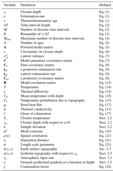
Table 1.Variables and location of definition in the text.
Variable Definition Defined
zc Closure depth Eq. (1)
˙e Exhumation rate Eq. (1)
τ Thermochronometric age Eq. (1)
∆T Time interval length Eq. (2)
M Number of discrete time intervals Eq. (2)
R Remainder ofτ/∆T Eq. (3)
Mmax Maximum number of discrete time intervals Eq. (4) N Number of ages Eq. (5)
A Forward model matrix Eq. (5)
ǫ Uncertainty on closure depth Eq. (6)
σ2
pr a priori variance Eq. (7) C Model parameter covariance matrix Eq. (7)
Cǫ Data covariance matrix Eq. (8) ˙epo a posteriori exhumation rate Eq. (9) ˙epr a priori exhumation rate Eq. (9) Cpo a posteriori covariance matrix Eq. (8) R Model resolution matrix Eq. (12)
T Temperature Eq. (14)
κ Thermal diffusivity Eq. (14)
Tm Mean temperature with depth Eq. (15) Td Temperature perturbation due to topography Eq. (15) ql Basal heat flux Eq. (17)
kl Thermal conductivity Eq. (17)
t∗
Onset of exhumation Eq. (17)
Tc Closure temperature Sect. 2.2 zm Closure depth with respect to z=0 Sect. 2.2 h Sample elevation Sect. 2.2
ψ2 Misfit criterion Eq. (19) ρ(u) Spatial correlation Eq. (21)
u Separation distance Eq. (21)
φ Length scale parameter Eq. (21)
h(x,y) Earth surface topography Sec. 3.3
p(x,y) Isotherm topography with respect to zm Sect. 3.3 γa Atmospheric lapse rate Sect. 3.3
γ General geothermal gradient as a function of depth Sect. 3.3
ζ Continuation factor Eq. (24)
the case where Mmaxis greater than N, the problem is non-unique. Even if N is greater than Mmax, the calculations of Eq. (6) will rarely be independent, so we must use formal inverse methods for underdetermined or mixed-determined problems. We use a method of linear Gaussian inversion in which both the unknowns (i.e., model parameters) and data are described as stochastic, or random, variables that have a Gaussian probability density characterized by a mean and a variance. Using this approach requires some a priori knowl-edge of the model parameters in order to construct a covari-ance matrix for the model parameters (Backus and Gilbert, 1968, 1970; Jackson, 1972; Tarantola and Valette, 1982).
In our case, the stochastic variables are the exhumation rate and the errors on the closure depth. Therefore, we define an a priori exhumation rate model that is independent of the data and consists of an estimate of the mean exhumation rate, ˙epr, and an estimate of the variance about this mean,σ2
elements equal to the a priori varianceσ2 pr:
Ci j=σ2prδi j, i,j∈[1,Mmax], (7)
whereδi j is the Kronecker delta. Off-diagonal elements of C are equal to zero as we assume exhumation rates are not
correlated in time. We then use the estimate of data errors,ǫ,
to describe the data covariance matrix, Cǫ, with dimensions N×N. In our problem, the errors in the system come from
analytical errors in the ages,εi, and from uncertainty in how
this relates to a closure depth. If the errors are uncorrelated, the data covariance matrix is diagonal, with components
(Cǫ)i j=
˙eprεi if i=j
0 if i,j (8)
Given this formulation of the model parameter and data co-variance matrices and the a priori estimate of the model pa-rameters, the underdetermined problem has a maximum like-lihood estimate of the model parameters (Franklin, 1970; Tarantola, 2005):
˙epo=˙epr+CAT
ACAT+Cǫ −1
(ˆzc−A˙epr), (9)
where ˙epr is a vector of length N containing the ˙epr. The model parameter estimate, ˙epo, is the maximum likelihood
estimate or the a posteriori exhumation rate. It is also treated as a Gaussian variable with a covariance matrix, Cpo, which
provides a measure of the uncertainty on the parameter esti-mate with respect to the a priori variance and is calculated as
Cpo=C−HAC, (10)
where the diagonal elements of Cpo show the a posteriori variance,σ2po, and H is the inverse operator from Eq. 9:
H=CATACAT+Cǫ −1
. (11)
One advantage of linear inverse methods is that one can es-timate the resolution of the inferred model parameters. The model resolution matrix, R
R=HA, (12)
provides a measure of this resolution. This resolution ma-trix gives information on how well the estimate of the model parameters correspond to the true parameters, and is a func-tion of the age distribufunc-tion and age uncertainty. R relates the difference between the a priori and a posteriori exhumation rates to the difference between the a priori and the actual, or true model parameters, ˙etrue, through
˙epo−˙epr=R(˙etrue−˙epr). (13)
If the resolution is perfect, ˙epo−˙epris equal to ˙etrue−˙epr. Per-fect resolution is obtained when the resolution matrix is equal to the identity matrix. In this instance, the exhumation rates inferred for a specified time interval are resolved indepen-dently of exhumation rates in other time intervals. The fur-ther R is from the identity matrix, the less resolved the model parameters are.
2.2 Computation of closure depth
Deriving an exhumation rate from thermochronological data requires information on the depth to the closure temperature. This can be achieved by solving the heat transfer equation:
∂T
∂t −˙e
∂T
∂z =κ∇
2T, (14)
where T (x,y,z,t) is the temperature, t is time, ˙e is the ex-humation, andκis the thermal diffusivity. Heat production is not explicitly included. However, as we calibrate model heat flow to measured surface heat flow, the contribution of heat production to near-surface geothermal gradients is accounted for. The surface boundary condition is the fixed temperature of the Earth’s surface and there is a basal condition reflecting the deep Earth heat flux.
For the thermochronometry problem the two effects we need to consider are perturbation of the isotherms by surface topography and vertical advection of heat by surface erosion and the upward motion of rock. We deal with each of these separately by decomposing the thermal field into two com-ponents (Turcotte and Schubert, 1982): an average temper-ature, Tm, which varies with depth and time, and a pertur-bation away from this mean induced by the topography, Td,
T (x,y,z,t)=Tm(z,t)+Td(x,y,z,t). (15)
The one-dimensional problem to solve for the mean temper-ature with depth is described by the simpler form of the heat equation:
∂Tm
∂t −˙e
∂Tm
∂z =κ
∂2Tm
∂z2 , (16)
which we solve using a finite difference method in space. The solution in time is obtained using a Crank–Nicolson time integration. We use an integration time step that provides a Courant–Friedrichs–Lewy number of∼1 to ensure accuracy.
The upper surface for the thermal model, z=0, is chosen as the average elevation, with respect to sea level, of the area covered by the data and the temperature at this elevation is T0. The boundary conditions are thus,
∂Tm) ∂z z=l
=ql kl Tm z=0
=T0,
(17)
where l is the depth to the base of the model, ql is the heat
flow into the base of the model, and kl is the thermal
con-ductivity. The initial condition for the problem (i.e., at time t∗
The next step consists of deriving the closure temperature and its corresponding closure depth from the thermal model. The closure temperature depends on the cooling rate at the time of closure (Dodson, 1973). We use kinetic parameters for the Dodson equation from the literature: helium diffusion in apatite (Farley, 2000), fission track annealing in apatite (Ketcham et al., 1999) and helium diffusion in zircon (Rein-ers et al., 2004). For an exhuming rock, the appropriate cool-ing rate is obtained from a transient geotherm through the material derivative:
DTm Dt =
∂Tm
∂t +˙e
∂Tm
∂z . (18)
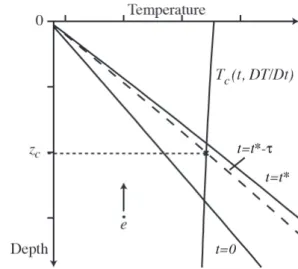
This cooling rate is then used to predict the closure temper-ature. With a transient geotherm Tm(t,z), cooling rate is a function of depth and time, but for any given time, there is a single depth where the temperature and the closure tempera-ture are equal (Fig. 1). The distance traveled by a rock from this depth to the surface is the closure depth and is equal to zm+h, where h is the elevation of the sample with respect to the mean elevation.
In order to calculate Tm(t,z), and thus cooling rate and clo-sure temperature, we require the exhumation rate. This is un-known and is the quantity that we are trying to obtain. This defines a nonlinear problem in ˙e, which we solve by direct iteration of Eq. (6). Fortunately, for most exhumation rates, this nonlinearity is weak and necessitates only a few itera-tions. We initialize the problem by using the a priori value for the exhumation rate, ˙epr.
2.3 Age elevation profile
The inversion scheme outlined above is now illustrated with a vertical age profile, where the AER can be easily interpreted. We use published apatite fission track (AFT) data from sam-ples collected within the footwall of the Denali Fault, taken from Fitzgerald et al. (1995) (Fig. 2). These data show a break in slope of the AER, which can be interpreted as a change in exhumation rate. Our aims are to assess how well we can resolve this apparent change in exhumation rate and to determine the dependencies of our inferred exhumation rates on (1) the time interval length,∆t; (2) the thermal pa-rameters; and (3) the a priori model for the exhumation rate. To assess the quality of fit of the predicted to the observed ages for the different models, we report a misfit criterion,ψ2, defined as
ψ2(˙e)= v u t 1 N
N
X
i=1
τpred,i−τi ǫi
!2
, (19)
where predicted ages,τpred, are calculated from the T−t paths
using Dodson’s expression, as described above. In the exam-ples below we present the misfit values for the ages using both the a priori and a posteriori model parameters. These
Figure 1.The evolution of crustal temperature through time in the presence of erosion rate at a rate of ˙e. Closure temperature, Tc, is shown at time t∗−
τ(Dodson, 1973). The initial geotherm (t=0) has a constant gradient. A cooling age ofτrecords closure at a time of, t=t∗−
τ, and a depth of, zc.
are designatedψ2
prandψ2po, respectively. The difference be-tween these numbers provides a quantitative measure of the model fit relative to the fit provided by a model with a con-stant exhumation rate.
We first describe results of a reference inverse model and then develop subsequent models by systematically varying parameterizations and a priori assumptions.
2.3.1 Reference inverse model
We start this reference model at a time equal to 25 Ma and discretize the exhumation history into time intervals,∆t, of 2.5 Myr. All elevations and depths are calculated with re-spect to a mean elevation of 4020 m. The thermal bound-ary condition is also fixed at this elevation, which is held at a temperature of−12◦
C. We assume an a priori exhuma-tion rate of 0.5±0.15 km Myr−1. The initial geothermal gra-dient is 24◦
C km−1. With a constant exhumation rate of 0.5 km Myr−1, the present day surface geothermal gradient would be 38.9◦C km−1. Values for other parameters used in the reference model are shown in Table 2.
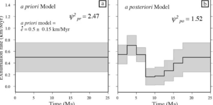
Solving Eq. (9) for the age data shown in Fig. 2 gives the exhumation estimate shown in Fig. 3. The solid line gives the inferred exhumation rate and the grey shaded region gives this rate plus or minus one standard deviation, which we ob-tain as the square root of the diagonal terms of the a posteriori covariance matrix, Eq. (10). The a posteriori data misfit,ψ2
po, is smaller than the a priori misfit,ψ2
pr, reflecting the improved data fit.
Table 2.Parameters used to determine reference inverse model for the Denali Fault in Sect. 2.3.1.
Parameter Value Units
hm 4020 m.a.s.l
T0 −12
◦ C
ql 76 mW m
−2
κ 30 km2Myr−1
kl 2.6 Wm
−1K−1
l 80 km
t∗
25 Ma
∆t 2.5 Myr
¯˙epr 0.5 km Myr −1
σpr 0.15 km Myr
−1
Figure 2.Apatite fission track ages from Mount Denali (Fitzgerald et al., 1995) plotted as a function of elevation. There is a break in slope at 6 Ma, interpreted as a response to an increase in exhuma-tion rate. The lower curve shows the evoluexhuma-tion of the closure depth through time in response to changes in the geotherm, as discussed in the text. Also plotted are the predicted ages (crosses) using the exhumation rate history shown in Fig. 3b.
rate. For these time intervals, the a posteriori variance is equal to the a priori variance, indicating that the data have no influence on the a posteriori rate. Subsequently, the cooling ages resolve a slow exhumation rate (with reduced variance) of about∼0.2 km Myr−1from 15–7.5 Ma and a high rate of 0.6 km Myr−1from 7 Ma to the present day.
During the iterative process the computed closure temper-atures and closure depths evolve subject to the exhumation rate. As shown in Fig. 4, the computed closure temperatures and closure depths with respect to the mean elevation remain constant after three iterations.
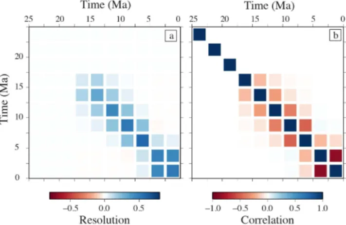
It is also important to establish the resolution of the in-ferred exhumation rate history. To this end, we calculate and show the resolution matrix R, Eq. (12), in Fig. 5a. It shows
Figure 3.(a) The a priori exhumation rate and (b) the a posteriori exhumation rate, which is variable in time. Grey envelopes indicate one standard deviation in the a priori or a posteriori exhumation rate. Also given are a norm of the misfit values to the ages using the a priori model and the a posteriori model,ψ2
prandψ2po, respectively.
that parameters relating to the early stages of the model (25–22.5 to 20–17.5 Ma) are unresolved, indicated by val-ues of zero in the upper left-hand block of the matrix. This is expected as there are no age data within these time intervals. The exhumation rate from 17.5 Ma to the present is partially-to-fully resolved by the data, reflected by the range of the measured ages. The highest value of resolution is the diago-nal element of the matrix corresponding to the time interval of 7.5–5 Ma. This corresponds to the high gradient segment of the AER, so that there are several ages within this interval constraining its exhumation rate. This is also reflected in the near zero values of the off-diagonal components of this row of the matrix. The most recent phase of exhumation, from 5 to 0 Ma, includes two time intervals (last two rows of the res-olution matrix). No ages fall into this time interval, and the exhumation rate for these two intervals is not well-resolved, as indicated by the near equal values of the four lower-right components of the resolution matrix. This shows that the ex-humation rate between 5 Ma and the present cannot be re-solved into two independent time intervals.
A further measure of parameter resolution is provided by assessing the covariance between model parameters. The full posterior covariance matrix provides that information. We scale covariance by the diagonal entries of the posterior co-variance matrix to assess the correlation, thereby providing a correlation parameter that varies from−1 to 1. We convert
covariance between two parameters,ξandβ, denoted Cξβ, to correlation between these parameters ˆCξβ(Tarantola, 2005):
ˆ
Cξβ= p Cξβ Cξξ
p Cββ
. (20)
Figure 4.Evolution of closure temperature and closure depth dur-ing the iterative process. The black circles show a sample collected from high in the vertical profile with an age of 9.2 Ma. The grey circles show a sample from lower elevations with an age of 5.2 Ma. Both ages show that after three iterations closure temperature and closure depths remain constant during the iteration process.
Anti-correlation is also expected: if two time intervals are available to exhume a rock from a given depth, by increas-ing the exhumation rate durincreas-ing one interval, the rate durincreas-ing the other interval is required to decrease. In the early stages of the model (25–22.5 to 20–17.5 Ma), the correlation matrix suggests that the model parameters are perfectly resolved. However, this is because the a posteriori covariance matrix is equal to the a priori covariance matrix, which is diagonal. In the time intervals younger than 17.5 Ma, the relative im-portance of negative off-diagonal elements is lowest during the 7.5–5 Ma time interval as this parameter has the high-est resolution. Conversely, the off-diagonal elements during more recent exhumation, from 5 to 0 Ma, have values close to minus one. These large negative values demonstrate that the most recent phase of exhumation is unresolved.
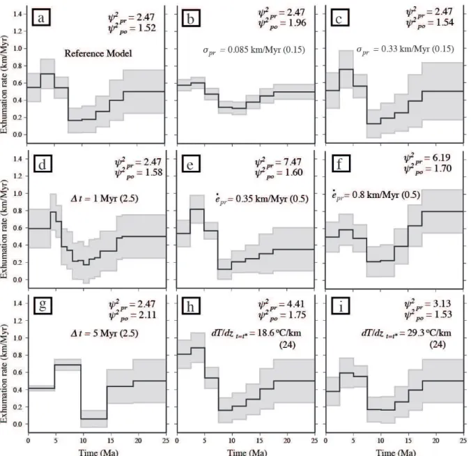
2.3.2 Effect of the time interval length
The inferred exhumation rates vary with the selection of the time interval length,∆t. Figures 6d and 6g show inversion re-sults where the time interval length has been changed relative to the reference model. In the case of shorter time intervals (Fig. 6d), the a posteriori standard deviation of the exhuma-tion rate is generally larger than that of the reference model in Figure 6a. The exhumation history is also more poorly re-solved. In spite of the fact that there is more generality to the exhumation rate history, the data misfit is increased andψ2
po is slightly higher compared to Fig. 6d. This is because, by having shorter, less well resolved time intervals, deviations from the a priori value are reduced and changes in exhuma-tion rate are smoothed. Finally, the timing of the change from slow exhumation to fast exhumation is approximately 7 Ma. This age of increased exhumation rate is very similar to age of the break in slope of the AER (see Fig. 2).
With longer time interval length the a posteriori standard deviation of the exhumation rate is reduced. This is because there are fewer model parameters and, therefore, fewer possi-ble exhumation rate histories that could fit the data. However,
Figure 5.The model resolution matrix (a) and the correlation ma-trix (b) for the inversion shown in Fig. 3. Each element in these matrices relates exhumation rate during one time interval to ex-humation rate during a different time interval. Large positive val-ues of the diagonals of the resolution matrix indicate well-resolved parameters.
ψ2
po is larger than for the reference model. This is due to the fact that the long time intervals changes in exhumation rate may not be possible at the appropriate time. For example, the time interval 10–5 Ma spans the break on slope (∼7 Ma) and
therefore the data fit is reduced.
The diagonal elements of the resolution matrices provide information about how well resolved exhumation rates are through time. For the reference model, a maximum resolu-tion value is found for the time interval of 7.5–5 Ma (and is∼0.6). With shorter time intervals, exhumation rates are
not resolved independently of one another and the maximum value is only 0.3. Conversely, with long time intervals the maximum resolution value is 0.97 for the time interval 5– 0 Ma, indicating that this parameter is almost perfectly re-solved.
This example highlights the trade-offbetween model com-plexity and variance reduction or parameter resolution. A greater number of time intervals permits greater variability and thus the precise timing of changes in exhumation rate to be identified. However, variance reduction and parameter resolution are decreased, indicating that model parameters are not resolved independently.
2.3.3 Effect of the thermal model
in-version results shown in Fig. 6h and 6i. In these models, the thermal parameters were selected such that the initial geothermal gradients are 18.6◦
C km−1and 29.3◦
C km−1, re-spectively, compared to the reference model, which has a gradient of 24◦
C km−1. In each case, we observe that when the exhumation rate is constrained by the vertical separation between two ages, the a posteriori exhumation rate estimate changes little. However, exhumation rates during the most re-cent stages vary widely, depending on the thermal model. For example, the inferred exhumation rate during the final time interval is 0.4 km Myr−1 for the case in which the surface geothermal gradient is relatively high (Fig. 6i), compared to 0.8 km Myr−1for the case with a low gradient (Fig. 6h).
2.3.4 Effect of changes in the a priori exhumation rate The a priori exhumation rate includes the expected value (mean) of exhumation rate and its variance. First, we inves-tigate the effect of changing the a priori variance, which acts as a penalty parameter. A lower variance forces the inverse solution to attain a value close to the a priori value of ex-humation rate. Conversely, a higher a priori variance permits more variation in the inverse solution, resulting in a better fit to the data. This is shown in Fig. 6b and c where the a priori variance is decreased and increased compared to the reference inverse model (Fig. 6a), respectively. With a lower a priori variance, a smoother solution is obtained as model parameters are penalized more strongly for deviations away from the a priori value. On the other hand, a large a priori variance (Fig. 6c) produces larger variations in the a poste-riori model parameters. In addition, the a pposte-riori variance has an important effect on the a posteriori variance. Therefore, in order to interpret the a posteriori variance as parameter un-certainty it is important to compare it to the a priori variance. Second, we explore the effect of the a priori mean exhuma-tion rate on the parameter estimaexhuma-tion. The cases in which the a priori exhumation rate is lower and higher are shown in Fig. 6e and f, respectively. In these models, the time intervals with no age constraints (17–25 Ma) simply have the a priori value of exhumation rate. However, once the ages constrain the exhumation rate, the a priori value has little influence on the a posteriori exhumation rate. It is also worth noting that we use the a priori exhumation rate to calculate the evolu-tion of the thermal model, which explains the observed dif-ferences in exhumation rates in Fig. 6a, e and f.
3 Inversion of spatially distributed data
Here we extend the previous analysis to account for ther-mochronometric data that are spatially distributed and there-fore have the potential to resolve spatial variability in ex-humation rate. We illustrate the methodology with a case study using topography and published data from the Dabie Shan, China.
3.1 Correlation in Space
We include spatial variability in exhumation rate by describ-ing exhumation rate as a spatial stochastic process. As a spa-tial stochastic process, a variable is described by not only a mean value and a variance but also by a spatial covariance. We thus define the covariance of exhumation rate, C, as a spatial process with a spatial correlation function. The corre-lation function describes how exhumation rates vary in space. We define this as a function of the separation distance, u:
ρ(u)=exp(−(u/φ)k), (21)
whereφ is a length scale parameter, and the function is a Gaussian function when k=2 and an exponential function when k=1.
3.2 Inverse Problem
The inversion process is constructed in the same manner as outlined for the co-located samples. However, we now define an independent exhumation history for each sample but re-quire that exhumation rate varies smoothly in space through the spatial correlation function. Hence, exhumation rate, ˙e, has length MmaxN and the forward model operator, A, has size N×MmaxN. The covariance matrix now contains the
spa-tial correlation structure between the exhumation rates de-fined in Eq. (21) (Tarantola and Nercessian, 1984; Willett, 1990). For a single time interval, a block of the covariance matrix is constructed using the separation distance between the ith and jth data (u) and the correlation function,ρ(u):
Ci j=σ2prδi jρ(u). (22)
It is assumed that exhumation rate is not correlated in time, so there is an independent matrix of form Eq. (22) for each time interval. These can be combined into a global matrix, setting cross time interval terms to zero.
Aside from this change in definition of the covariance ma-trix, the inversion process and the definition of the inverse op-erator, Eq. 9, remain unchanged. The a posteriori covariance matrix contains information about how inferred rates covary in time and space. The resolution matrix contains informa-tion about which parameters are determined independently of one another in time and space.
We have introduced a new model parameter, the charac-teristic length scale,φ. Its value can either be prescribed in a way to give a desired spatial smoothing, or it can be estimated through geostatistical methods (e.g., Matheron, 1963). The value ofφprovides a means to trade-offmodel smoothness against variance reduction. A smallerφreduces the number and weight of age data used to infer exhumation rates at any given location. A largerφprovides more spatial smoothing.
Figure 6.Exhumation rates inferred from age data from Fitzgerald et al. (1995) for different a priori model parameters. (a) Reference model; (b–i) independent analyses with one parameter changed with respect to the reference model, as indicated. The corresponding parameter value in the reference model is shown in brackets.
weighted average of the exhumation rates evaluated at the data locations. Here the relative weights are defined by the separation distances between the data locations and the point of interest and the correlation function imposed in the inver-sion.
The resolution matrix still relates the estimated and true values of exhumation rate but now includes temporal and spatial relationships. As a consequence, R is difficult to visu-alize. To simplify, we integrate the resolution values across the spatial dimension for each time interval. An integrated value of one corresponds to an exhumation rate that is re-solved independently of other time intervals.
3.3 The effects of topography on a closure isotherm In Sec. 2.2 we calculated the depth to a closure isotherm from a one-dimensional model that assumed an isothermal bound-ary condition at the mean topographic elevation. However, if we are to extend the analysis to investigate exhumation rates across a larger region, the topography of Earth’s sur-face needs to be included (Lees, 1910; Bullard, 1938; Jef-freys, 1938; Birch, 1950; Werner, 1985).
topography and surface temperature to perturbations of tem-perature on a horizontal plane located near the Earth’s sur-face. This temperature perturbation at the surface can then be propagated downwards to a specific depth, zm. In turn the per-turbation in temperature at a specific depth can be converted to a perturbation in depth of an isotherm (Turcotte and Schu-bert, 1982; Stüwe et al., 1994; Mancktelow and Grasemann, 1997).
In Eq. (15) we decomposed the temperature field into two components, a mean temperature that varies with depth, Tm, and a perturbation from this mean, Td. Mancktelow and Grasemann (1997) derive an expression to calculate temature perturbations at depth due to a cosine tempertemature per-turbation at the surface in the presence of heat advection. In our notation this expression is
Td(λ,z) z=z
m=exp(ζzm)Td(λ,z)
z=0, (23)
where Td(λ,z)
z=0, is a cosine function with known wave-length,λ, andζis defined as
ζ=−
˙e 2κ+
s ˙e
2κ
2
+(2πk)2
, (24)
where k is the wave number (1/λ).
However, the depth perturbation of a closure isotherm is required and not simply the temperature perturbation at a specific depth calculated from the thermal model, Tm, as in Sect. 2.2. As closure depth evolves through time due to the advection of heat, the mean closure depth for each ther-mochronometric system is used to calculate a perturbation for each system.
The elevation of the surface of the model is chosen as the mean elevation of the area covered by the analysis. A temper-ature perturbation at this elevation is a function of the pro-jection of the surface temperature (surface topography and atmospheric lapse rate) and the local geothermal gradient (Bullard, 1938; Jeffreys, 1938),
Td(λ,z)
z=0=−h(λ)(γ0−γa), (25)
where h(λ) is cosine function representing Earth’s topogra-phy andγa is the atmospheric lapse rate.γ0 is the geother-mal gradient at z=0 taken from the transient mean thermal model, Tm, and the specific time in the past.
Similarly, the temperature perturbation at a mean closure depth, zm, can be written in terms of the isotherm topography and the geothermal gradient at that depth,γzm:
Td(λ,z)
z=zm=−p(λ)γzm, (26)
where p(λ) is the perturbation of the closure isotherm about zm. At this point we have expressions for Tdat z=0 as a func-tion of the topography that can be easily calculated, and Tdat z=zmas a function of the topography of a closure isotherm. These expressions, Eq. (26) and Eq. (25), can be combined in
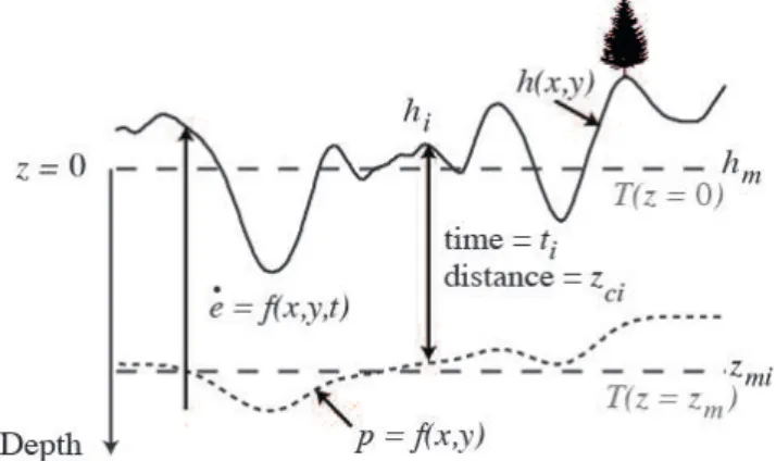
Figure 7.Surface topography, h, and a closure isotherm, p. The mean elevation, hm, is defined relative to sea level, but subsequent depths and elevations are taken from this datum, thus defined to be
z=0. The mean closure depth zmi, calculated for a specific age i, is shown as long dashed line, and p is the closure isotherm. An age,
τ, from elevation, hi, records the time taken to exhume from the closure depth, zci.
Eq. (23) to give the perturbation of closure depth. The result-ing expression for a specific wavelength of the topography, h(λ), is
p(λ)=A0exp(ζzm)h(λ), (27)
where A0contains the atmospheric lapse rate and geothermal gradients evaluated from Tm,
A0= γ0−γa
γzm !
. (28)
Finally, as any complex topography in one or two dimensions can be described as a infinite sum of periodic functions, and the principle of superposition applies, this analysis can be extended to account for any topography. We calculate p(x,y) in the frequency domain (e.g Ducruix et al., 1974; Black-well et al., 1980; Blakely, 1996). The distance to a closure isotherm for a single age is given by
(zc)i=(zm)i−pi+hi (29)
where piis the value of p(x,y) at the spatial location of the
age, as illustrated in Fig. 7.
4 Case study from the Dabie Shan, SE China
Figure 8.(a) Topographic map of the Dabie Shan, SE China, showing zircon (U-Th)/He, apatite fission track and apatite (U-Th)/He ages in blue triangles, orange circles and yellow diamonds, respectively, from Reiners et al. (2003). (b) The ages plotted as a function of elevation.
zircon (ZHe) and from apatite (AHe), and AFT dating (Rein-ers et al., 2003). The ages across the region show a posi-tive AER in the core of the range and older ages around the flanks (Reiners et al., 2003). They concluded that exhuma-tion rate has been slow, 0.06±0.01 km Myr−1, since the
Cre-taceous, with a possible increase in exhumation rate (up to 0.2 km Myr−1) between 80–40 Ma. There appear to be few tectonic structures responsible for this observed pattern of cooling ages, suggesting decay of old topography. Braun and Robert (2005) attributed the exhumation pattern to an iso-static response of relief reduction in the core of the range.
We use the Dabie Shan topography and data distribution to demonstrate and validate two key components of our inver-sion methodology: first, the approximation for the influence of topography on a closure isotherm; and second, the impor-tance of the correlation structure of the parameter covariance matrix. As a test of the inversion scheme, before applying the algorithm to the measured ages, we apply the analysis to a suite of known synthetic ages produced with a thermo-kinematic model.
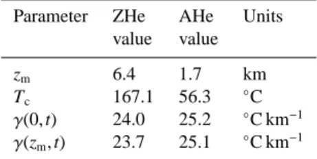
4.1 Example of the closure isotherm approximation We use the topography of the Dabie Shan to demonstrate how the perturbation of a closure isotherm is calculated. The mean closure depths for AHe and ZHe are estimated from a one-dimensional thermal model representative of the Dabie Shan, Tm. The upper boundary of the thermal model is set at the av-erage elevation, inferred from SRTM data (Farr et al., 2007), over the region shown in Fig. 9, 149.1 m.a.s.l.; the tempera-ture at this elevation is set and held at 14.1◦
C. Other param-eters used in the thermal model are defined in Table 3. This
initial model results in geothermal gradient of 22.7◦
C km−1, which increases to 25.3◦
C km−1after 120 Myr of erosion at 0.06 km Myr−1.
From Tm we obtain the average values for the parameters required to calculate the closure isotherms, Table 4.
The topography with respect to the mean elevation of the area is shown in Fig. 9a. The two-dimensional discrete Fourier transform of the topography is computed using stan-dard methods (e.g., Press et al., 1992) and we compute p(x,y) in the frequency domain. The perturbation of the closure isotherms of AHe and ZHe about the mean closure depths are shown in Fig. 9b and 9c, respectively.
4.2 Testing the closure isotherm approximation
The analytical method for calculating the topographic ef-fects on isotherm depth involve a number of approximations, foremost of which is the conversion of the Earth’s surface into a temperature perturbation on a flat plane. To compare the perturbation of an isotherm about a mean depth, we ini-tially calculate a value for the mean depth and temperature, as in Sect. 2.2. We also calculate Tm by applying a con-stant temperature at depth 900◦
C at z=31.5 km so that the models are compatible. We evaluate a mean closure depth using Tm for AHe closure at the mean age of AHe ages,
τAHe=40.9 Ma, at a temperature of 57.44◦
C. To test our ap-proximation for the thermal structure of the crust we generate a three-dimensional thermal field, using a finite-element so-lution to the advection–conduction equation, Pecube (Braun, 2003). Using identical thermal parameters and the topo-graphic surface, the depth of the 57.44◦
Table 3.Parameters used to calculate the temperature field for the Dabie Shan, as described in Sect. 4.1.
Parameter Value Units
hm 149.1 m.a.s.l
T0 14.1
◦ C
κ 35 km2Myr−1
kl 2.6 Wm
−1K−1
l 51.5 km
t∗
120 Ma
¯˙epr 0.08 km Myr −1
method presented in Sect. 3.3. The misfit in depth between the isotherms calculated with the two different approaches is small,−1.68 m.
4.3 Testing resolution of the data
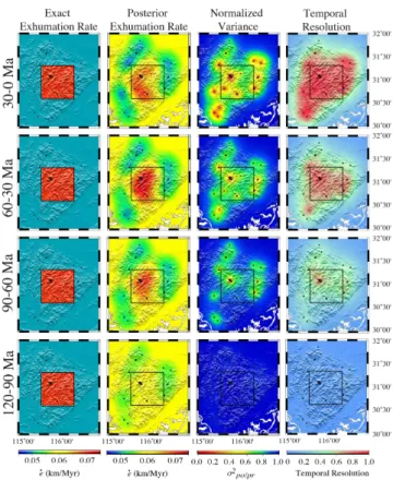
In this section, we conduct a resolution test to see how well the data from the Dabie Shan could be expected to resolve a spatially variable exhumation pattern. This test is made by generating synthetic age data from a known exhuma-tion funcexhuma-tion, then analyzing these data with our inversion scheme in order to see how well the known exhumation rates are recovered. The procedure provides a confirmation of our inversion algorithm, but is primarily a test of the resolving capability of the Dabie Shan data number and location.
Synthetic ages are produced by integrating the temperature along material paths in the 3-D finite-element code Pecube (Braun, 2003). We specify a vertical velocity with an ex-humation rate of 0.07 km Myr−1 within a rectangular region in the center of the model domain and 0.05 km Myr−1 out-side of this rectangle. We predict AHe, AFT and ZHe ages with the Dodson approximation, at the same spatial locations as in Reiners et al. (2003). We assign the same measurement errors as in the reported data.
For the inversion analysis, we used an a priori exhumation rate of 0.06 km Myr−1with an a priori standard deviation of 0.02 km Myr−1. We used an exponential spatial correlation function with a length scale parameter of 28 km, although we investigate the effects of this parameter later. The time interval length for the model is 30 Myr. We use the same thermal parameters and boundary conditions as were used to generate the synthetic ages.
Figure 10 shows the resulting inferred exhumation rates. Results are shown for each of the four time intervals of the in-verse model. During the time interval from 120 Ma to 90 Ma, only the oldest ages influence the estimate of the exhuma-tion rate and these are all found in the peripheral, slow-exhumation rate region. We normalize the a posteriori vari-ance by the a priori varivari-ance as this provides a measure of the information content of the data. A normalized variance value of one and a temporal resolution value of zero high-lights where the model is not resolved. The normalized a
Table 4. Parameters used to calculate closure isotherms for the Dabie Shan, as described in Sect. 2.3.1.
Parameter ZHe AHe Units value value
zm 6.4 1.7 km
Tc 167.1 56.3
◦ C
γ(0,t) 24.0 25.2 ◦
C km−1
γ(zm,t) 23.7 25.1
◦ C km−1
posteriori variance and the temporal resolution show that the solution is poorly resolved during this time interval.
From 90–60 Ma, there are also age data within the block of fast exhumation rate, and near these data, the exhumation rate is partially resolved, as indicated by the reduction of the a posteriori variance and the increase of temporal reso-lution. By 60–30 Ma, the exhumation rate is resolved and ac-curately estimated; however, due to the smoothness imposed in the model covariance matrix, the distinct boundaries of the block are “blurred”. This pattern is also observed in the final time interval, 30–0 Ma; however, the exhumation rates are slightly lower than the true values in the core of the block. Where there is an absence of data, for example in the south-east corner, the exhumation rate never deviates from the a priori value and shows a normalized variance close to one, whereas values of temporal resolution remain close to zero, as shown in Fig. 10.
The blurred nature of the result is due to the smooth cor-relation function used for the parameter covariance matrix. With additional ages located close to the boundaries of the block, we would be more likely to resolve this discrete step in exhumation rate.
As a further complication, it is evident that the blurring in space during one time interval also influences the entire exhumation rate history for the region. The exhumation rate during the oldest time interval demonstrates this effect. Dur-ing this time interval there are only ages where the exhuma-tion rate is slow. These slow rates are correctly inferred out-side of the block, but are also inferred within the block. The degree to which exhumation rate outside of the block de-pends on exhumation rate within the block is a function of the correlation scale, and secondarily of the a priori variance; the larger the a priori variance, the easier it is for distant data to influence the result.
In addition, as this spatial averaging results in a low es-timate of exhumation rate in the block, the advective heat transport and geothermal gradients are also underestimated and closure depths overestimated. This effect is similar to the example shown in Sect. 2.3.3.
4.4 Effect of the correlation function
Figure 9.(a) The surface topography of Dabie Shan, (b) the topography of the closure isotherm for the AHe system and (c) the topography of the closure isotherm for the ZHe system. The isotherms are plotted as perturbations about the mean closure depths for the two systems. Refer to Sect. 3.3 and Sect. 4.1 for a full description.
length scale parameter, Eq. (21). Figure 11 shows how the a posteriori misfit,ψ2
po, changes as a function of the correlation length scale,φ. Two correlation functions are used, an expo-nential function and a Gaussian function. If the correlation length,φ, is low, in the extreme this becomes equivalent to inverting each age independently with no ability to average out noise in the data or to identify changes in exhumation rate through time. Furthermore, deviations of the a posteri-ori rate from the a priposteri-ori exhumation rate are suppressed (see Fig. 11). In contrast, whenφis large, samples which record different exhumation rates are forced to correlate and so an overly smooth exhumation pattern is obtained, as can be seen in Fig. 11.
4.5 Exhumation history of the Dabie Shan
We now apply our method to the measured ages of Reiners et al. (2003). As with the synthetic data, the model is ini-tiated at 120 Ma and the exhumation history is discretized into 30 Myr time intervals. The a priori exhumation rate is 0.08±0.03 km Myr−1based on Al-in-hornblende geobarom-eter estimates of intermediate calc-alkaline plutons and or-thogneisses from within the Dabie Shan (Ratschbacher et al., 2000). Our thermal model predicts an increase of surface geothermal gradients from the initial value at the onset of ex-humation, 22◦C km−1to the present day value of 25◦C km−1 through time (Hu et al., 2000). The closure depths are calcu-lated as described in Sect. 4.1. Prior to about 115 Ma, ex-humation rates were very high, ∼2 km Myr−1 (Liu et al., 2010), and may have perturbed the thermal regime, but we assume that this effect does not influence the late thermal history (Ratschbacher et al., 2000). We impose a correlation length scale parameter ofφ=28 km.
Estimated exhumation rates in space and time are shown in Fig. 12. During the time interval of 120–90 Ma, there is low spatial resolution due to the limited number of old ages (see Fig. 12). At the eastern end of the range (where the
ages are oldest), exhumation rates of∼0.09 km Myr−1are re-solved, as indicated by the low a posteriori variance. In the core of the range, the exhumation rates are slightly lower,
∼0.07 km Myr−1. The north and south flanks of the range are
not well resolved, as indicated by the high normalized vari-ance and low resolution values.
From 90–60 Ma we see high exhumation rates (>
0.1 km Myr−1) near the Tan-Lu Fault, and a gradual decrease towards the northwest, possibly supporting activity on this fault during this time interval (Grimmer et al., 2002). The northeastern extent of the range continues to exhume at
∼0.09 km Myr−1.
The time interval from 60–30 Ma shows slower exhuma-tion rates at the front of the range close to the Tan-Lu fault, in agreement with Reiners et al. (2003). There is also a de-crease in exhumation rate in the eastern region. In contrast, we observe a slight increase in the core of the range. This pat-tern of exhumation rate, with the core of the range exhuming faster than the flanks, is consistent with an isostatic response to a decrease in relief and reduction of topography.
During the final time interval of exhumation, 30–0 Ma, a similar structure as in the previous time interval is in-ferred, with the core of the range exhuming faster than the flanks. However, the magnitude of the exhumation rates has reduced, most noticeably in the core of the range from∼0.08
to∼0.06 km Myr−1.
5 Discussion
thermochronomet-Figure 10.Results of the inversion of synthetic data with locations at the black points; thermochronometric system of each datum is consistent with the measurements of Reiners et al. (2003). Each row corresponds to a different time interval. The red boxes in the left column define a region with an exhumation rate of 0.07 km Myr−1; background rate is 0.05 m Myr−1. The second column shows ex-humation rates inferred through inversion of these data. The third column shows the parameter variances normalized by the a priori variance. The right column displays the temporal resolutions.
ric systems, we resolve cooling rates in time by fitting the travel time between closure isotherms as well as final cool-ing to the surface.
The innovation of our method is that it combines many of the common methods of analyzing thermochronometric ages to derive exhumation rate. Least-squares fitting of ages dis-tributed in elevation, thermal modeling of depth between clo-sure temperatures for different mineral systems, and thermal modeling of individual ages can all be considered subsets of our analysis method. The problem with many of these tradi-tional methods is that one must assume that all the ages dis-tributed across a landscape have a common exhumation his-tory, which is often not the case. Here we address this prob-lem explicitly by imposing a spatial correlation, thereby re-quiring a common exhumation history only for points within a distance defined by a correlation length scale.
A major assumption of our method is that the kinetics of all thermochronometers are governed by a linear first order Arrhenius process, which enables us to use Dodson’s
ap-Figure 11.Sum of the squared misfit between predicted and ob-served ages as a function of the correlation length scale,φ. The gray circles show the results assuming an exponential correlation func-tion (k=1, Eq. (21)); the black circles use a Gaussian correlation function (k=2, Eq. (21)).
proximation to estimate the depth of closure. However, a large body of work shows that the kinetics of AFT or AHe can become nonlinear due to effects such as radiation dam-age or multi-compositional annealing (Carlson et al., 1999; Ketcham et al., 1999, 2007; Shuster et al., 2006; Flowers et al., 2009). Fortunately, expanding the use of Dodson’s pa-rameters to represent the kinetics of closure can still include some of these complexities. For example, where composi-tional information is available for AFT ages, specific popula-tions of ages can be modeled with specific sets of kinetic pa-rameters. In this case, retentive apatites and non-retentive ap-atites would be modeled with separate kinetic parameters and thus closure temperatures. Similarly, grain size or radiation damage in (U-Th)/He ages can be accounted for by redefin-ing the correspondredefin-ing first order kinetic parameters (Reiners and Brandon, 2006; Shuster et al., 2006). In the extreme case, defining specific kinetic parameters independently for each measured age is possible and would require no modifications to our method as defined here.
Figure 12.Exhumation rate history of the Dabie Shan. The left column shows the a posterior exhumation rates, the center column shows the a posteriori variances normalized by the a priori variance, and the right-hand column shows the temporal resolutions.
Our method is best used for regional studies where the exhumation history is relatively simple. This is, first, be-cause we assume that rocks only experienced monotonic cooling, implying that complex reheating has not occurred. Second, exhumation rates are smooth in space and are not strongly affected by surface-breaking faults. This latter com-plication can be easily accounted for, where these are well-identified, by building them into the correlation structure. In such cases, samples from either side of a fault could follow independent exhumation histories. In scenarios where ages record complex cooling and reheating histories, our approach would not be suitable because Dodson’s approximation is in-valid. Fortunately, complex cooling histories can be identi-fied through additional information such as the analysis of fission track length distributions (Gallagher, 1995; Willett, 1997; Ketcham et al., 2007; Gallagher et al., 2005).
The thermal model, although simpler than solving a full three-dimensional problem, includes the major components
Figure 13.Comparison between model-predicted ages and mea-sured ages. The solid black line is the 1 : 1 line. The error bars are the reported standard deviation of the measured ages.
of heat transfer necessary to solve this problem (i.e., conduc-tion and advecconduc-tion). This combined with a spectral method enables us to include the effects of topography on the shape of underlying isotherms. It should be successful in most cases, but it might fail in regions of very high relief or very high exhumation rates where the approximation of topogra-phy into temperatures on a plane might not be accurate. Fur-thermore, where exhumation rate is described by 2- or 3-D kinematics, our methodology may be less successful. For ex-ample, orogens with high rates of horizontal displacement, which is associated with large scale thrust faulting, should be treated with caution. Our implementation could lead to an apparent change in exhumation rate in time, which would correspond to a change in the trajectory of rocks traveling through an orogenic wedge or up a thrust ramp. Likewise, the thermal model that we have implemented will not account for exhumation in situations where extensional unroofing domi-nates, unless it is very shallow.
One of the advantages of the formal inversion we adopt is in the ability to assess noise propagation from data to model parameters and to establish resolution. As the results of the analysis vary due to changes in the imposed parameterization and thermal model, shown in Fig. 6, the inferred exhumation rate uncertainty (obtained from the a posteriori covariance matrix) does not reflect the true model uncertainty. There-fore, a range of models with different imposed parameteriza-tion are required to convey the true uncertainty. We focus on interpreting the resolution in time; spatial resolution can be inferred from the spatial distribution of an age data set. It is computed, by definition, using the data error and parameter covariance matrices and, in our case, integrated spatially. It indicates how well exhumation rates at each time interval can be resolved independently of exhumation rate in other time intervals. The examples we report clearly show that resolu-tion degrades back in time, which implies that we are more likely to resolve more recent exhumation rates and their vari-ations.
As the problem as we have defined it is underdetermined, we require additional information to determine exhumation rate. This is in the form of a mean exhumation rate, ˙epr, and an expected variance about this mean,σ2(along with a model for spatial covariance for the spatial case). In the majority of cases the a priori exhumation rate is an estimate of the aver-age exhumation rate derived from any available information, although in principle it should be independent of the ther-mochronometric data. This could be in the form of sediment flux into neighboring sedimentary basins, geodetic derived rock uplift rates, or paleo–barometry estimates. Additional complexities, in the form of spatial and temporal variations, could be built into the a priori exhumation rate. However, where data exhibit good elevation distributions, results are relatively independent of the a priori exhumation rate.
For the spatial case, the parameter covariance matrix we implement largely controls the spatial resolution. It is de-fined through a correlation length scale and an a priori vari-ance on the a priori exhumation rates. It serves as a trade-offparameter, trading solution resolution in space against the need to average out noise and to combine ages from differ-ent elevations or with differdiffer-ent closure temperatures in or-der to resolve exhumation rates in time. Therefore, it is key to choose a correlation length scale that is appropriate. In most cases, it can be defined using statistical methods, for example, through the computation of a semi-variogram (e.g., Matheron, 1963). Similarly, the a priori variance must be chosen carefully. Its primary influence is as a weighting fac-tor for the data uncertainty, and is chosen based on a trial-and-error approach.
Application of our method requires that exhumation histo-ries be discretized into a predefined, carefully chosen, num-ber of time intervals. Time interval lengths should be short enough to suitably represent the temporal variations of in-terest without attempting to infer too many model param-eters. With a short time interval length, parameter
resolu-tion is reduced and the a priori informaresolu-tion dominates. Con-versely, as the time interval length increases, parameter res-olution increases. However, the ability of the method to re-solve changes in exhumation rate decreases. Therefore, time interval length should be chosen based on the age distribu-tion.
6 Conclusions
The linear Gaussian inversion method presented here pro-vides a practical, yet powerful tool to convert age informa-tion into exhumainforma-tion rates. Our method generalizes the cor-related concept of travel–time from a closure depth to the Earth’s surface that is implicit in age–elevation relationships. In addition, it permits the simultaneous analysis of ages from different thermochronometric systems, provided their reten-tion characteristics can be expressed in terms of first-order kinetics.
In addition to providing an estimate of exhumation rates, the formalisms of inverse theory provide associated measures of the quality of the exhumation rate estimates. These are in the form of covariance and resolution matrices. These ma-trices show that data variance, their geographic locations, a priori knowledge of exhumation rate, and the temporal dis-tribution of the ages all play an important role in inferring exhumation rates.
We propose that our method is best suited to regional stud-ies, where a general model for space and time variations in exhumation rate is desired. Given that the approach is linear, and the isotherms are calculated using an analytical solution, we can efficiently estimate exhumation rates across a range of wavelengths and timescales.
Acknowledgements. We would like to thank Jean Braun and Peter van der Beek for stimulating discussions throughout the de-velopment of the work. Thanks to Mark Brandon for his help with the topographic perturbation to the closure isotherms. JeffMoore and Rebecca Reverman are thanked for reviews of the manuscript. Figures were prepared using the Generic Mapping Tools (Wessel and Smith, 1998).
Edited by: J. Braun
References
Backus, G. and Gilbert, F.: The resolving power of gross earth data, Geophys. J. Roy. Astron. Soc., 16, 169–205, 1968.
Backus, G. and Gilbert, F.: Uniqueness in the inversion of inaccurate gross earth data, Philosophical Transactions of the Royal Society of London, Series A, Mathemat. Phys. Sci., 266, 123–192, 1970. Batt, G. E. and Braun, J.: On the thermomechanical evolution of compressional orogens, Geophys. J. Internat., 128, 364–382, 1997.