www.earth-syst-sci-data.net/8/571/2016/ doi:10.5194/essd-8-571-2016
© Author(s) 2016. CC Attribution 3.0 License.
The PRIMAP-hist national historical emissions time
series
Johannes Gütschow1, M. Louise Jeffery1, Robert Gieseke1, Ronja Gebel1, David Stevens1, Mario Krapp2, and Marcia Rocha2
1Potsdam Institute for Climate Impact Research, Telegraphenberg A 31, 14473 Potsdam, Germany 2Climate Analytics, Friedrichstraße 231, Haus B, 10969 Berlin, Germany
Correspondence to:Johannes Gütschow ([email protected])
Received: 15 April 2016 – Published in Earth Syst. Sci. Data Discuss.: 2 June 2016 Revised: 7 October 2016 – Accepted: 12 October 2016 – Published: 9 November 2016
Abstract. To assess the history of greenhouse gas emissions and individual countries’ contributions to
emis-sions and climate change, detailed historical data are needed. We combine several published datasets to cre-ate a comprehensive set of emissions pathways for each country and Kyoto gas, covering the years 1850 to 2014 with yearly values, for all UNFCCC member states and most non-UNFCCC territories. The sectoral resolution is that of the main IPCC 1996 categories. Additional time series of CO2 are available for energy and industry subsectors. Country-resolved data are combined from different sources and supplemented us-ing year-to-year growth rates from regionally resolved sources and numerical extrapolations to complete the dataset. Regional deforestation emissions are downscaled to country level using estimates of the deforested area obtained from potential vegetation and simulations of agricultural land. In this paper, we discuss the data sources and methods used and present the resulting dataset, including its limitations and uncertainties. The dataset is available from doi:10.5880/PIK.2016.003 and can be viewed on the website accompanying this paper (http://www.pik-potsdam.de/primap-live/primap-hist/).
1 Introduction
The question of responsibility for climate change and its im-pacts plays a significant role in the UNFCCC1negotiations around the global agreement to limit the global mean temper-ature increase and avoid dangerous climate change. It is inter-linked with the discussion about equitable access to sustain-able development, which forms the basis of different frame-works to assess whether climate targets put forward by coun-tries reflect a “fair share” in the collective burden to reshape the economy towards emissions neutrality. The Brazilian del-egation to the UNFCCC has put forward a framework that assesses a country’s contribution to climate change by cal-culating the fraction of the total warming generated by that country’s historical greenhouse gas emissions. This approach is explained in Miguez and Filho (2000) and has been quan-tified in Höhne et al. (2010), den Elzen et al. (2013), and
1United Nations Framework Convention on Climate Change
Matthews et al. (2014), among others. Other effort-sharing proposals use cumulative per capita emissions as a metric and thus also need a detailed record of historical emissions by in-dividual countries (Winkler et al., 2011; Baer et al., 2008; Bode, 2004). In 2001 the MATCH2expert group was estab-lished by the UNFCCC to generate historical emissions time series for this purpose. The dataset which resulted from this effort proved very useful in the negotiations and to the scien-tific community (Höhne et al., 2010). It was updated in den Elzen et al. (2013) with data from the Emissions Database for Global Atmospheric Research v4.2 (EDGAR) to cover all gases and emissions until 2010. The Climate Analysis Indi-cator Tool (CAIT) also publishes a historical greenhouse gas emissions dataset that is a composite of other sources (World Resources Institute, 2016). However, non-CO2emissions are only covered for recent years (1990–2012) and it resolves
either sectors or gases but not both at the same time. Most of the sources used in the CAIT composite dataset are also included in the dataset presented here. The Global Carbon Project publishes the Global Carbon Budget (Le Quéré et al., 2015), which covers the atmospheric concentration of CO2 and its sources and sinks. The fossil fuel CO2emissions data used are taken directly from other sources; non-CO2 emis-sions data are not included.
Here we present a historical emissions dataset with a finer sectoral resolution, newly available input data, and new and improved methods for the combination of datasets. Previ-ous versions of the PRIMAP-hist (PRIMAP – Potsdam Real-time Integrated Model for probabilistic Assessment of emis-sions Paths) dataset have been used in the UNEP3gap report 2015 (UNEP, 2015) and the INDC fact sheets published by the Australian-German Climate and Energy College (Mein-shausen and Alexander, 2016). Predecessors of the dataset, especially the PRIMAP4 baseline4, have been used, for ex-ample, for the Climate Action Tracker5and in Meinshausen et al. (2015). The dataset presented here has been improved in categorical resolution, time coverage, and country cover-age compared to its predecessors. Methodological improve-ments include extrapolation with regional growth rates, more sophisticated downscaling methods (e.g., for land use emis-sions), and category and gas aggregation that automatically interpolates and extrapolates missing data.
We build our time series from a range of publicly available data sources (see Sect. 2), which are prioritized based on their completeness and reliability – an approach that has also been taken by the IPCC6to compile the historical dataset for the 5th Assessment Report (IPCC, 2014, Annex.II.9, Historical data). For each time series (country-, gas-, and sector- re-solved), the lower-priority sources are used as year-by-year growth rates7 to extend the higher-priority sources. Where no country data are available, we use regional growth rates, growth rates from superordinate sectors, and numerical ex-trapolation to complete the time series.
For land use emissions, we use the approach introduced in Matthews et al. (2014) and downscale a regional dataset using estimates of deforested areas derived from simulations of potential vegetation and agricultural land.
The PRIMAP-hist dataset covers the six Kyoto greenhouse gases and gas groups (Kyoto GHG). Independent time se-ries are generated for carbon dioxide (CO2), methane (CH4), nitrous oxide (N2O), hydrofluorocarbons (HFCs), perfluoro-carbons (PFCs), and sulfur hexafluoride (SF6). For all gases
3United Nations Environment Programme 4https://www.pik-potsdam.de/research/ climate-impacts-and-vulnerabilities/research/
rd2-flagship-projects/primap/emissionsmoduledocumentation/ primap-baseline-reference
5http://www.climateactiontracker.org 6Intergovernmental Panel on Climate Change 7Other publications use the term “rate of change”.
except CO2, the sectoral resolution is that of the main IPCC 1996 categories. For CO2, more detailed categories are used because some important datasets cover only subsectors of categories 1 and 2. For details and sector names, we refer the reader to Table 1.
NF3 is not included as it has only been included in the group of Kyoto Protocol relevant gases for the second com-mitment period of the Kyoto Protocol, which started in 2013, and data availability is therefore still scarce. In the remainder of the paper we use the term fluorinated gases to refer to the combined group of gases HFCs, PFCs, and SF6.
We use the IPCC 1996 categories instead of the new IPCC 2006 categories because almost all data sources are reported using the 1996 categories and we can avoid conversions be-tween categorizations by using the 1996 categories. The UN-FCCC is switching towards IPCC 2006 categories for data re-ported by countries; however, issues with the reporting soft-ware resulted in some countries delaying their emissions re-porting and others asking the UNFCCC not to display the reported data. We plan to switch to the IPCC 2006 categories for a future release of the PRIMAP-hist dataset once these problems are solved.
The emissions time series cover the period of 1850 to 2014. This is achieved through the combination of various sources and extrapolation for some sectors, gases, and coun-tries both into the past and into the future. The extent of the extrapolation needed varies between sectors, gases, and countries. Data coverage is very good for energy-related CO2 emissions for the whole period. For other gases and sectors we have to rely on growth rates from regional data for the period before 1970 and on numerical extrapolation for the period after 2012. The data sources we use are described in Sect. 2, while the details of the combination process, includ-ing the prioritization, are described in Sect. 4.
The time series starts in 1850 for all sectors, including land use. Pre-1850 land use emissions have a small effect on cu-mulative emissions, and accounting for them would “results in a shift of attribution of global temperature increase from the industrialized countries to less industrialized countries, in particular South Asia and China, by up to 2–3 %” (Pon-gratz and Caldeira, 2012). On the other hand, uncertainties are especially high for early emissions, which limits the use-fulness of the additional data. However, preindustrial land use change emissions could be included in a future version of this dataset.
Table 1.Categorical detail of the PRIMAP-hist source for different gases. The categorical hierarchy uses IPCC 1996 terminology. The subcategories of categories 1 and 2 are only resolved for CO2. Other gases are treated at the level of categories 1 and 2. For categories 2E and 2F of the industrial sector, there are no data for CO2because these categories only include the production and consumption of fluorinated gases.
Category Sector name Gases
0 National total CO2, CH4, N2O, HFCs, PFCs, SF6
0EL National total excluding LULUCF CO2, CH4, N2O, HFCs, PFCs, SF6
1 Total energy CO2, CH4, N2O
1A Fuel combustion activities CO2, CH4, N2O 1B1 Fugitive emissions from solid fuels CO2
1B2 Fugitive emissions from oil and gas CO2
2 Industrial processes CO2, CH4, N2O, HFCs, PFCs, SF6
2A Mineral products CO2
2B Chemical industries CO2
2C Metal production CO2
2D Other production CO2
2G Other CO2
3 Solvent and other product use CO2, N2O
4 Agriculture CO2, CH4, N2O
5 Land Use, land use change, and forestry CO2, CH4, N2O
6 Waste CO2, CH4, N2O
7 Other CO2, CH4, N2O
to the state the territory currently belongs to. Emissions of former colonies are thus attributed to the now independent state and not to the former metropolitan state. Occupation of countries’ territories is only taken into account if the oc-cupying country reports the emissions from that territory.8 In Sect. 4.3 we present a list of territories included in the emissions of UNFCCC parties as well as information on the territories that are treated separately and how we deal with missing data and territorial changes.
The paper is organized as follows: we begin by describing the individual data sources we use in Sect. 2 and their pri-oritization in Sect. 3. In Sect. 4 we describe how the dataset is constructed from the individual sources, including the spe-cial treatment of land use data. In Sect. 5 we give information on how to obtain and use the data. Results are described in Sect. 6 with information on the uncertainties of emissions data in Sect. 7. Limitations are covered in Sect. 8. Method-ological details and data sources that we did not use are de-scribed in the Appendices A, B, and C.
2 Data sources
In this section we describe the data sources used to create our composite source. We only use sources that are publicly available and give preference to sources that are not com-posites of other sources in order to avoid including original sources twice, once directly and once indirectly, through a composite source. However, it is likely that some sources
8This is the case for Israel and the Palestinian territories, for example.
share at least some input data, such as information on fossil fuel production or use the same emission factors. The sources are grouped into four categories.Country-reported dataform
the highest priority category as it can benefit from detailed knowledge about the specific situation in a country and is well accepted in the context of the UNFCCC negotiations. This is exemplified by the linking of the entry into force of the Paris Agreement to the latest country reported emissions and not to any third-party source (UNFCCC, 2015b). Where this data are not available, or do not meet our minimum re-quirements (see Sect. 2.1 below), we usecountry-resolved dataprovided by third parties, such as research institutions
and international organizations. To extrapolate data into the past we use region-resolved datasets. Finally, we use two
gridded datasetsto calculate land use change patterns and
subsequently country-resolved land use change emissions. Figure 1 gives an overview of the data sources described in detail in the remainder of this section. Detailed information on data preprocessing is available in Appendix B. In the text we refer to data sources using the abbreviations introduced in the source description below.
2.1 Minimum requirements for data
1850 1900 1950 2000
RCP
EDGARHYDE14 HOUGHTON
BP2015 EDGAR42 FAO2015 land use FAO2015 agriculture CDIAC2015 UNFCCC2015 BUR2015 CRF2013 CRF2014
All countries Global data Regional data Annex I countries Non-Annex I countries
Figure 1.Coverage of years and countries in the sources used for the PRIMAP-hist dataset. The color indicates the country group covered or the regional resolution, while the intensities indicate the fraction of countries in the group covered by the source in each year. The fraction is taken over all gases and categories, which can be seen in the CDIAC time series, where the flaring time series only starts in 1950. The RCP time series for CH4ends in 2000, leading to the lower coverage after the year 2000.
extend a higher-priority source (for details see Sect. 4.1 and Appendices A4 and A5). To weaken the influence of these fluctuations, we use the trend of several years for the match-ing instead of a smatch-ingle year. We therefore require that each time series contain at least three data points spread over a period of at least 11 years. Furthermore, we need time series with the detail of sectors and gases listed in Table 1.
2.2 Country-reported data
Under the UNFCCC there are several requirements for re-porting of greenhouse gas emissions data (see, e.g., Yamin and Depledge, 2005). Both developed (Annex I) and devel-oping (non-Annex I) parties9have to regularly submit com-munications that include an inventory of national GHG emis-sions and removals. Detailed requirements, however, differ strongly between Annex I and non-Annex I parties. An-nex I parties have to submit an inventory that covers all sec-tors, gases, and years since 1990 annually. The submissions should consist of two parts, the common reporting format (CRF) tables with the data and a national inventory report (NIR), which gives background information like the rationale
9The term “parties” refers to the countries which have ratified the UNFCCC. Annex I parties refers to those countries listed in Annex I of the Kyoto Protocol (KP) which are the developed coun-tries under the UNFCCC. The definition is now almost two decades old and does not represent the state of economic development any more. The distinction between developed and developing countries is thus subject to constant debate in the UNFCCC meetings.
behind the selection of emission factors and methodological questions. For details on the CRF tables, see Sect. 2.2.3 be-low. Annex I parties also submit national communications, which originally served the purpose to report on policies and measures to implement the party’s commitment to aim to re-turn emissions to 1990 levels by the year 2000. The NIRs have recently (decided in 2011 at COP1710, Durban, South Africa) been complemented with biennial reports to enhance reporting. The emissions data contained should be consistent with the CRF data. Under the Kyoto Protocol (KP), Annex I parties have to regularly submit information needed to assess whether they are meeting their emissions targets. For our pur-pose, the CRF data are the most useful of these sources. The other sources do not provide additional information for the purpose of this paper and are not used.
Non-Annex I parties were required to submit an initial na-tional communication within 3 years after the entry into force of the convention. The least developed countries (LDCs) could decide whether to submit an initial national commu-nication. The submissions were required to contain an emis-sions inventory which covers the years 1990 to 1994 for most submissions. A time frame for subsequent national commu-nications could not be agreed upon, and only a few countries submitted further national communications with updated in-ventories. The guidelines for national communications for non-Annex I parties are less stringent than the guidelines for Annex I parties; consequently, the coverage and detail in sec-tors and gases of the data differ strongly between countries. Since 2014, non-Annex I parties have been required to report GHG inventory information through biennial update reports (BURs). The first report was due by December 2014; how-ever, only 24 of over 150 countries have actually submitted (as of January 2016). LDCs and SIDS11 (94 countries in to-tal) are exempted from the mandatory submission and can submit at their discretion.
The Paris Agreement requires regular national inventory reports by all parties, which might improve emissions report-ing in the future (UNFCCC, 2015b, Article 7(a)).
2.2.1 National communications and national inventory reports for developing countries (UNFCCC2015)
Most developing countries reported historical emissions data at least once using national communications (UNFCCC, 2015a) and sometimes national inventory reports. However, several countries only reported data for the period of 1990 to 1994, sometimes only single years. Therefore, a lot of countries’ submissions do not meet our minimal data re-quirements and are consequently not used for the compos-ite source. Where the data meet our requirements, we use them with high priority as they are prepared by in-country ex-perts, which gives the results based on these data high
ibility within the country and is beneficial for policy anal-ysis. We compare the data with third-party data to identify whether there are differences that cannot be explained by un-certainties. National inventory reports give a more detailed overview over the emissions inventory than national com-munications but are not published by all countries. While developed-country parties also submit national communica-tions and national inventory reports we only use these data for developing countries as we have the CRF data for devel-oped countries (see Sect. 2.2.3 below). The data used here have been downloaded from the UNFCCC website using the “Detailed data by party” interface (UNFCCC, 2015c). The date of access was 25 September 2015. Some countries sub-mit their data prepared according to IPCC 2006 guidelines. These data are not available through the interface (Andorra, Cook Islands, Jamaica, Kiribati, Malawi, Mauritania, Mex-ico, Namibia, Samoa, Swaziland, South Africa, and Tunisia). Furthermore, the UNFCCC greenhouse gas data interface seems to lag behind the submissions and misses some sub-missions from 2015 and 2016 (as of 1 February 2016). The source preprocessing is explained in Appendix B.
2.2.2 Biennial update reports (BUR2015)
Biennial update reports (BURs) are submitted to the UN-FCCC by non-Annex I parties (UNUN-FCCC, 2016). They con-tain greenhouse gas emissions information with varying de-tail in sectors, gases, and years. As of 1 February 2016, 24 countries have submitted data. Unfortunately, most of the submissions do not meet our minimal data requirements.
Argentina, Ghana, India, Namibia, Paraguay, Peru, Thai-land, Tunisia, and Vietnam have submitted detailed values only for a single year. Bosnia and Herzegovina has published data for 2010 and 2011. Andorra and Macedonia have pub-lished only aggregate Kyoto greenhouse gas data.
Brazil and Singapore have published detailed information for 1994, 2000, and 2010; however, the level of detail is not sufficient for all sectors. Chile, Mexico, South Africa, Re-public of Korea, and Uruguay have detailed information for a range of years in the annex to the BUR and the NIR. How-ever, for South Africa the level of detail is not sufficient for all sectors and gases.
Colombia, Costa Rica, and Montenegro use the IPCC 2006 categorization, so we cannot include the data in the current version of this dataset. The Lebanon BUR was not accessible on the UNFCCC website, so we could not assess whether there are useful data in it (as of 1 February 2016).
The final PRIMAP-hist dataset uses BUR2015 data for Azerbaijan, Brazil, Chile, Republic of Korea, Mexico, Singa-pore, South Africa, and Uruguay. The source preprocessing is explained in Appendix B.
2.2.3 UNFCCC CRF (CRF2014, CRF2013)
CRF data, short for common reporting format, are reported by all Annex I parties every year on a mandatory basis. The data are very detailed, both in sectors and gases, and undergo review for consistency and compliance with reporting guide-lines by expert teams from the UNFCCC roster of experts. We use the final version of the 2014 data (UNFCCC, 2014a), which contains information until the year 2012. The 2013 re-vision (UNFCCC, 2013) is used as a backup in case there are gaps in the 2014 data. The first year is 1990 with a few exceptions of data series starting in 1985. All Kyoto gases are covered and data are submitted using IPCC 1996 cate-gories.12
The 2015 edition of the CRF data uses IPCC 2006 cate-gories. This posed problems in data preparation for several countries such that publication was significantly delayed. To date (April 2016), not all countries have submitted their data, with large emitters missing.13 The gas NF
3has been added as it is included in the Kyoto greenhouse gases for the second commitment period of the Kyoto Protocol. CRF2015 data will be included in a future update of this dataset together with a move to IPCC 2006 categorization.
Appendix B contains some additional information on the creation of the emissions pathways with individual fluori-nated gases combined together.
2.3 Country-resolved data
2.3.1 BP Statistical Review of World Energy (BP2015)
The BP Statistical Review of World Energy is published ev-ery year and contains time series for CO2 emissions from consumption of oil, gas, and coal (which corresponds to IPCC 1996 category 1A). Emissions data are derived on the basis of the carbon content of the fuels and statistics of fuel consumption. The 2015 edition (British Petroleum, 2015) contains information for 76 individual countries and 5 re-gional groups of smaller countries, which we downscale to country level. The first year in the time series is 1965, and the last is 2014. Appendix B gives details on the downscaling. We use the BP data additionally to sources covering similar gases and categories (e.g., CDIAC) because they offer emis-sions data for recent years which are not included in the other sources.
2.3.2 CDIAC fossil CO2(CDIAC2015)
The CDIAC fossil fuel and industrial CO2emissions dataset is published by the Carbon Dioxide Information Analysis 12When we write “all” there can still be a few exceptions where data are missing for single countries or sectors.
Center (CDIAC) with regular updates (Boden et al., 2015). It covers emissions from fossil fuel burning, flaring, and ce-ment production for 221 countries and territories. The first year is 1751 and the last year 2011. Emissions from 1751 to 1949 are computed using statistics of fossil fuel production and trade combined with information on the chemical com-position of the fuels and assumptions on the use and combus-tion efficiency following the methodology presented in An-dres et al. (1999). Emissions data for the years 1950 to 2011 are based primarily on the United Nations Energy Statis-tics Yearbook (United Nations, 2016) using the methodol-ogy presented in Marland and Rotty (1984). The data require some preprocessing to account for division and unification of countries. The preprocessing methodology and mapping of emissions categories are explained in Appendix B.
2.3.3 EDGAR versions 4.2 and 4.2 FT2010 (EDGAR42)
The EDGAR14 dataset is published by the European Com-mission Joint Research Centre (JRC) and Netherlands Envi-ronmental Assessment Agency (PBL). It undergoes regular updates. The current (1 February 2016) version is 4.2. It con-tains emissions data for all Kyoto greenhouse gases as well as other substances.15It covers 233 countries and territories in all parts of the world, though not all countries have full data coverage. EDGAR version 4.2 covers the period 1970 to 2008 (JRC and PBL, 2011). Additionally the EDGAR v4.2 FT2010 covers the period 2000 to 2010 (JRC and PBL, 2013; Olivier and Janssens-Maenhout, 2012). EDGAR v4.2 FT2012 covers 1970 to 2012 but only for CO2, CH4, N2O, and aggregate Kyoto GHG emissions with no sectoral resolu-tion (JRC and PBL, 2014; UNEP, 2014). Version 4.3 cover-ing the period until 2012 has been implicitly announced but is not yet available (as of 1 February 2016).16
EDGAR time series are calculated using activity data on a per sector, per gas, and per country basis. Emissions are cal-culated using a country, sector, and gas-specific technology mix with technology-dependent emission factors. The emis-sion factors for each technology are determined by end-of-pipe measures, country-specific factors, and a relative emis-sion reduction factor to incorporate installed emisemis-sions re-duction technologies.
Appendix B contains information on the combination of EDGAR v4.2 and EDGAR v4.2 FT2010, as well as details on the category and gas basket aggregation and country pre-processing.
14Emissions Database for Global Atmospheric Research 15Some of the other substances in the EDGAR database are con-trolled under the Montreal Protocol (HCFCs), while others are not yet controlled (e.g., black carbon, organic carbon).
16In the “Trends in Global CO
2emissions report” (Olivier et al., 2015), EDGAR v4.3 is referenced as forthcoming in 2015.
2.3.4 FAOSTAT database (FAO2015)
The Food and Agriculture Organization of the United Na-tions (FAO) publishes data with yearly values for emissions from agriculture and land use (Food and Agriculture Organi-zation of the United Nations, 2015a). Over 200 countries and territories are included in the database.
The land use emissions are categorized into forestland, grassland, cropland, and biomass burning, where the first three categories contain information on CO2 only, while biomass burning also contains information on N2O and CH4 emissions. To generate the time series, data from land use and forestry databases (both from FAO and other institutions) are used together with IPCC estimates of emission factors and the FAO “Global Forest Resources Assessment” database for carbon stock in forest biomass. For details we refer the reader to the methodology information on the FAOSTAT website (Food and Agriculture Organization of the United Nations, 2015b). The time series cover 1990 to 2012.
The land use emissions do not cover the emissions directly introduced by agriculture, but emissions from soil changes that are caused by agricultural use of the soil. For cropland FAOSTAT states that “greenhouse gas (GHG) emissions data from cropland are currently limited to emissions from crop-land organic soils. They are those associated with carbon losses from drained histosols under cropland.” (Food and Agriculture Organization of the United Nations, 2016).
FAOSTAT data for agricultural emissions range from 1961 to 2012. They cover N2O and CH4 from various sources (e.g., rice cultivation, synthetic fertilizers, and manure man-agement). Because the data cover a longer time period than other sources for the agricultural sector, we use them with highest priority after the country-reported data. The data are generated from activity data and emission factors following the tier 1 approach of the IPCC 2006 guidelines.
Appendix B gives details on the emissions categories and country processing.
2.4 Regionally resolved datasets
2.4.1 Houghton land use CO2(HOUGHTON2008)
trop-ical regions from 1990 onward are estimates (constants17). For our dataset the regional emissions have to be downscaled to country level. This is described in Sect. 4.2.2, while tech-nical details are given in Appendix B.
The dataset covers only direct (deliberate) human-induced activities (Houghton, 2003, 1999). Thus, generally, forest fires are not included except for fire clearing. However, wild-fires and the effect of measures for fire suppression are in-cluded for the USA.
We use this dataset as a proxy for CO2 emissions from land use, land use change, and forestry (LULUCF) as land cover change accounts for the majority of LULUCF emis-sions (Smith et al., 2014).
2.4.2 RCP historical data (RCP)
The representative concentration pathways (RCPs) were cre-ated for the CMIP5 intercomparison study of Earth system models that was organized by the World Climate Research Programme and used (among other models) in the IPCC’s Fifth Assessment Report (AR5). They have a common his-torical emissions time series that covers all Kyoto gases but is only resolved at a coarse regional and sectoral level (Meinshausen et al., 2011b). For N2O and fluorinated gases, only economy-wide global emissions are available. For CO2, global emissions are split into land use and fossil and indus-trial emissions. CH4emissions are resolved into five regions with several subcategories of the IPCC 1996 categorization.
RCP historical data are compiled from a wide range of emissions sources and atmospheric concentration measure-ments. Where concentration data are used, inverse emis-sions estimates are computed using the MAGICC6 reduced-complexity climate model (Meinshausen et al., 2011a). RCP historical data can be used for extrapolation of country time series to the past using regional growth rates. RCP land use emissions data are not used in our dataset as they are based on the Houghton dataset, which we include directly (see previ-ous section). Preprocessing of RCP data is explained in Ap-pendix B.
2.5 EDGAR-HYDE 1.4 (EDGAR-HYDE14)
The EDGAR-HYDE 1.4 “Adjusted Regional Historical Emissions 1890–1990” dataset covers the gases CO2, N2O, and CH4for the years 1890 to 1995 (Olivier and Berdowski, 2001; Van Aardenne et al., 2001). The data are given for 13 regions, some of which are individual countries (USA, Canada, Japan). They are generated from the EDGAR v3.2 dataset (Olivier and Berdowski, 2001) and the “Hundred Year Database for Integrated Environmental Assessments” (HYDE v1.1) (Van Aardenne et al., 2001; Goldewijk and
17The constant emissions outside tropical regions are obtained using the assumption that emissions calculated for 1990 are also valid for the subsequent years.
Battjes, 1997). We use the EDGAR-HYDE dataset to extrap-olate country emissions into the past. It has a relatively high sectoral detail, but the sectors differ from the IPCC 1996 def-initions, so mapping to IPCC 1996 sectors is necessary. De-tails are presented in Appendix B.
2.6 Gridded datasets
The two gridded datasets included in the generation of the PRIMAP-hist dataset do not contain any emissions data. In-stead, they contain data for potential vegetation and simula-tion data of past existing vegetasimula-tion. By comparing these, we can determine areas where deforestation has occurred, which we use to downscale the Houghton land cover change emis-sions data to country level. More information on the use of these datasets is provided in Sect. 4.2.2.
2.6.1 HYDE land cover data (HYDE)
The HYDE land cover data (Klein Goldewijk et al., 2011, 2010; PBL, 2015) are generated using hindcast techniques and estimates on population development over the last 12 000 years. For the time period of interest here, they pro-vide estimates of pasture and crop land on a 5 arcmin resolu-tion grid for 10-year time steps. The data do not directly pro-vide estimates for deforestation, but these can be computed by comparison with simulation data of potential vegetation (e.g., from SAGE; see below).
2.6.2 SAGE Global Potential Vegetation Dataset (SAGE)
This dataset is available in the SAGE18 database and is de-scribed in Ramankutty and Foley (1999) and available for download from Ramankutty and Foley (2015). It contains 5 arcmin resolution grid maps of potential vegetation (i.e., vegetation that potentially could be in a certain spot if there was no human interference) for a time period from 1700 to 1992. It has been used together with HYDE 3.1 in Matthews et al. (2014) to downscale CDIAC land use CO2emissions to country level. We use it for the same purpose here.
3 Source prioritization
To create a dataset covering all countries and gases for a pe-riod of over 150 years, multiple data sources need to be com-bined as no single source contains all the necessary data. We order sources such that the highest-quality sources are se-lected for each gas, category, and year, according to avail-ability. Where possible, source prioritization is defined, and used, at a global level.
The source creation is carried out such that the abso-lute values are taken from the highest priority source, while
lower-priority sources are used as year-to-year growth rates to extend the time series. The prioritization of the sources takes the completeness and reliability of the absolute values into account to use the most reliable absolute values and the year-by-year growth rates of the other sources to extend those data. A similar method is employed for the Global Carbon Budget (Le Quéré et al., 2015), where the motivation is that the growth rates are less uncertain than the absolute values. The details of the process of the combination of sources are described in Sect. 4.
3.1 Emissions from energy, industrial processes, solvent use, agriculture, and waste
For fossil emissions, our highest priority source is the UN-FCCC CRF data as they are both accepted by the coun-tries that report and by other councoun-tries because they are re-viewed by experts. However, these data are only available for developed-country parties. We use CRF2014 and fill gaps with CRF2013 where necessary. For non-Annex I parties we use data from national communications and national inven-tory reports with highest priority (UNFCCC2015). For a few developing countries, data from the biennial update reports (BUR2015) are available and fulfill our minimal require-ments. These are used to supplement the UNFCCC2015 data. UNFCCC2015 is prioritized over BUR2015 because the lat-ter only contains a few data points for most countries, while the UNFCCC2015 data contain full time series for more countries. These sources of UNFCCC-reported data cover a wide range of gases and sectors. For most countries, CO2, CH4, and N2O are available for all sectors at the level of de-tail needed for the composite source. Fluorinated gases are only contained for a few countries. For CO2 related to fos-sil fuel burning, CO2from flaring, and CO2emissions from mineral products, we use CDIAC as the next priority source. For CO2from other sectors and all other gases we use a com-bination of EDGAR v4.2 FT2010 and EDGAR v4.2 as the next priority source.This combined EDGAR dataset is also used to complement CDIAC data where necessary (e.g., for small countries missing in the CDIAC source). BP2015 data are used to extend the energy CO2 time series until 2014. Where no reported data are available, the country-resolved data sources are used as the first sources.
Sources without country-level information, i.e., RCP and EDGAR-HYDE, are used to extrapolate emissions into the past. As EDGAR-HYDE has a higher regional and sectoral resolution it is used as the first priority source for extrapola-tion of CO2, CH4, and N2O emissions. Emissions from flu-orinated gases for years before 1970 are only available from the RCP historical data and only on a global level.
The source prioritization for the individual gases is sum-marized in Tables 2, 3, 4, and 5. Details of the source creation methods are available in Sect. 4.1.
3.2 Land use, land use change, and forestry emissions
The first priority source for land use CO2is FAOSTAT. How-ever, it does not contain information for the period before 1990. EDGAR42 does contain information starting in 1970 but excludes sinks from the calculation of CO2land use emis-sions, which is why we exclude EDGAR CO2land use data from our dataset. The period before 1990 is covered by the Houghton dataset on a regional level, which we downscale using estimates of historical deforestation (see Sect. 4.2).
For CH4 and N2O we use country-reported data, FAO-STAT, and EDGAR data on a per country basis. Regional growth rates from EDGAR-HYDE14 are used to extrapolate the time series.
Details of the source creation are presented in Sect. 4.2 and in Tables 6 and 7 within that section.
4 Dataset construction
4.1 Emissions from energy, industrial processes, solvent use, agriculture, and waste
The generation of the emissions time series is carried out us-ing the composite source generator (CSG) of the PRIMAP emissions module described in Nabel et al. (2011). Data are aggregated on a per country, per gas, and per category level taking into account source prioritization (see Sect. 3). The result is one time series for each country, category, and gas. The source creation is organized in the four steps described below.
Source preprocessing First, each dataset undergoes
source-specific preprocessing, e.g., category mapping and country preprocessing, which is explained in Ap-pendix B. This is followed by category aggregation: if data are defined on a more detailed level of gases (in the case of HFCs and PFCs) or categories (e.g., cate-gories 4A and 4B), they are aggregated to the resolu-tion described above for all sources individually. The aggregate time series covers the union of all years of the individual gas or sector series. If data are missing for some years in any of the individual gas or subcate-gory time series, they are interpolated to close gaps and extrapolated to fill missing data at the boundaries before aggregation. After aggregation, the information that a subcategory or gas was missing is lost. If data are miss-ing at the gas and category level we are workmiss-ing with in the PRIMAP-hist dataset, they are not interpolated in preprocessing as they can be filled from other sources.
Composite source generator The composite source
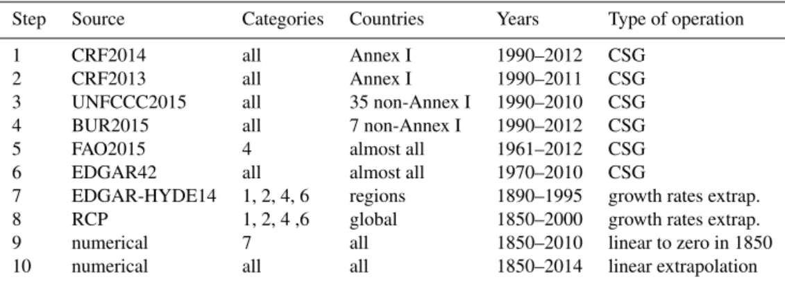
lower-Table 2.Source prioritization and extrapolation for fossil and industrial CO2. In Fig. 3 we show the individual steps using the example of category 1 for the Republic of Korea. Years are maximal values. Some countries have less coverage. In CRF a few countries have data starting a few years before 1990. Category names refer to IPCC 1996 categories.
Step Source Categories Countries Years Type of operation
1 CRF2014 all Annex I 1990–2012 CSG
2 CRF2013 all Annex I 1990–2011 CSG
3 UNFCCC2015 all 35 non-Annex I 1990–2010 CSG
4 BUR2015 all 8 non-Annex I 1990–2012 CSG
5 CDIAC2015 1A, 1B2, 2A almost all 1850–2011 CSG
6 EDGAR42 all almost all 1970–2010 CSG
7 BP2015 1A almost all 1965–2014 CSG
8 EDGAR-HYDE14 1A, 1B1-2, 2A-G regions 1890–1995 growth rates extrap.
9 RCP 1A global 1850–2005 growth rates extrap.
10 PRIMAP-hist CAT1A all but 1A all 1850–2014 growth rates extrap.
11 numerical all all 1850–2014 linear extrapolation
Table 3.Source prioritization for fossil and industrial CH4. Years are maximal values. Some countries have less coverage. In CRF a few countries have data starting a few years before 1990. Category names refer to IPCC 1996 categories. Note that there are no CH4emissions data in category 3 (solvent and other product use).
Step Source Categories Countries Years Type of operation
1 CRF2014 all Annex I 1990–2012 CSG
2 CRF2013 all Annex I 1990–2011 CSG
3 UNFCCC2015 all 35 non-Annex I 1990–2010 CSG
4 BUR2015 all 7 non-Annex I 1990–2012 CSG
5 FAO2015 4 almost all 1961–2012 CSG
6 EDGAR42 all almost all 1970–2010 CSG
7 EDGAR-HYDE14 1, 2, 4, 6 regions 1890–1995 growth rates extrap.
8 RCP 1, 2, 4 ,6 global 1850–2000 growth rates extrap.
9 numerical 7 all 1850–2010 linear to zero in 1850
10 numerical all all 1850–2014 linear extrapolation
priority sources. After this step the priority algorithm fills gaps in the time series using lower-priority sources and extrapolates using year-to-year growth rates from lower-priority sources. The composite source time se-ries for each gas, category, and country is checked for gaps and whether or not it covers the full time period. If that is the case, the second-highest priority source is checked for data that could fill gaps and extend the time series. If that time series itself contains gaps or needs extension, the default behavior of the CSG is to parse the hierarchy downwards recursively and to use the re-sulting time series to extend the composite source. For this study we add one source at a time and therefore do not parse the sources recursively but rather add what is present in the next priority source and then see whether the resulting time series needs further extension. For de-tails on the harmonization of the lower-priority sources, see Appendix A4. If there are data missing after the end of this process, the CSG can numerically interpolate gaps and extrapolate missing data at the boundaries. For this dataset we only use the interpolation by the CSG,
because we use regional growth rates from other sources to extrapolate the country data. A schematic of the com-posite source generator within the PRIMAP emissions module is shown in Fig. 2.
The rationale underlying this combination method is that the absolute values are taken from the highest pri-ority source, while lower-pripri-ority sources are only used for the dynamics of emissions. By scaling the lower-priority sources to match the higher-lower-priority source, we retain the year-to-year growth rates of the lower-priority sources but adjust the absolute values to the highest pri-ority source. For details see Appendix A4. Other options for harmonization are discussed in Sect. 8.
Extrapolation Missing years in the past are extrapolated
EDGAR42
CRF2014 CDIAC2015
UN2012 RCP
FAO2015
...
PRIMAPDB Preprocess
* Translate to common sector terminology * Downscale if neccessary * Aggregate sectors and gases
Prioritize sources
Select and prioritize sources
Copy missing countries
Copy missing countries / regions to composite source if available in lower priority sources
Start compsource
Start composite source with a copy of the highest priotity source
Calculate or copy missing categories
If categories are missing (1) aggregate sub-categories or (2) copy, if available in lower priority sources
Inter- and extrapolate over time (priority alg.)
Complete the composite source time series by using growth rates from lower priority data
Extrapolation
Extrapolate time series using regional data or numerical methods.
Composite Source
Figure 2.The composite source generator (CSG) is used to assem-ble time series from different sources into one time series covering all countries, sectors, gases, and years. The source prioritization in the figure is illustrative and does not represent the source prioriti-zation for the dataset described here. In this study the internal cate-gory aggregation of the composite source generator is not used, but categories are aggregated before the generation of the composite source to enable extrapolation of subcategories. For the PRIMAP-hist dataset we always combine only two sources at a time instead of recursively filling missing data. Section 4.1 and Appendix A de-scribe the use of the CSG for this dataset. Figure 3 shows the indi-vidual steps for an example time series.
for longer periods. We also offer a dataset without this numerical extrapolation.
When using extrapolation with growth rates from re-gions or other sectors, we make the assumption that these time series share growth rates with the unknown time series we want to determine through extrapolation. This assumption seems crude, but it is much more trans-parent than, for example, building a more complicated model to compute the time series. A more sophisticated model will likely also need some input data, such as population or economic data, to estimate an extrapo-lated time series. Such input data are also scarce for the time periods we need the extrapolation for (i.e., be-fore 1960/1970). Numerical extrapolation, on the other hand, does not require any information for the time pe-riod for which we want to build our time series, and it only uses data from a range of years before or after the time period to be computed. It thus makes the as-sumption that we can deduce emissions in one time pe-riod from emissions in another time pepe-riod, which is of-ten not true. As an example, consider the Second World War, when emissions changed drastically, and that a nu-merical extrapolation would not model when using, for example, 1960–1980 as input data. However, a regional time series for Europe, for example, would have this
feature and would model emissions for European coun-tries more realistically than numerical extrapolation. We still use numerical extrapolation for the PRIMAP-hist dataset, but only when it is the only option because no national or regional data exist.
Postprocessing After extrapolation the individual gas and
category time series are aggregated to build the higher categories and the Kyoto GHG basket. For details on the aggregation, see Appendix A1.2.
Sudan needs a special treatment as the split into Sudan and South Sudan was so recent that no separate emis-sions data are available yet. We downscale the Sudan emissions time series to Sudan and South Sudan us-ing UN population statistics (UN Population Division, 2015) as a downscaling key. We also aggregate country data for some regional groups.
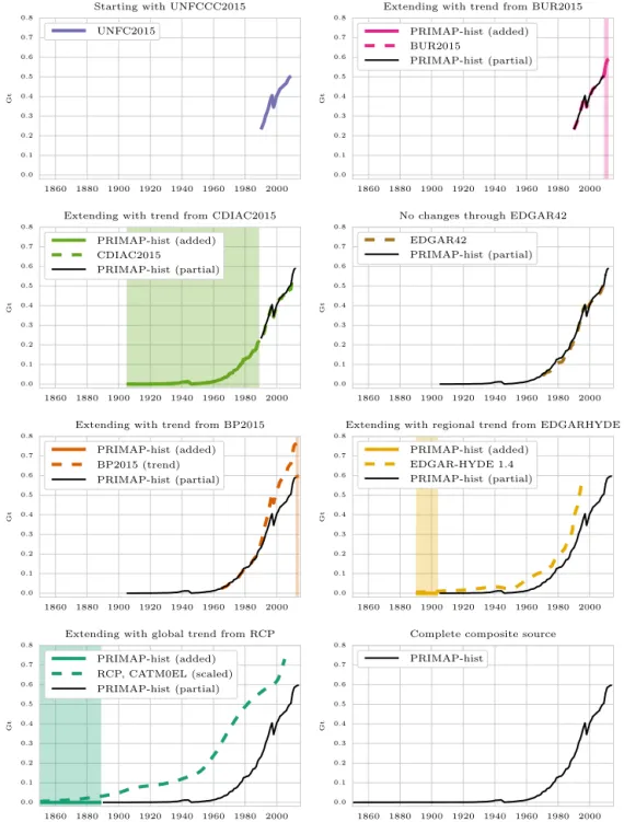
Figure 3 shows an example of how we build a pathway from different time series.
In the following we describe the availability and use of datasets in detail for the different gases and sectors.
CO2 Data coverage for CO2 is, in general, very good. The largest emissions sources are the consumption and production of fossil fuels and the production of ce-ment. Both are covered by CDIAC, which extends the country-reported data back to 1850 for 31 countries, to 1900 for 65 countries, to 1950 for 168 countries, and to 1990 for 196 countries. For other sectors EDGAR42 extends the time series back to 1970. BP data complete the fossil fuel consumption time series until 2014. To further extend time series into the past we use EDGAR-HYDE regional growth rates (starting in 1890). For categories 1A, 1B1, and 1B2, explicit time series are available, while we use category 2 time series as a proxy for the subcategories of category 2. Other categories are not available. RCP CO2data that range back until 1850 are only available for total emissions excluding LULUCF on a global level. As total CO2 emissions are dominated by fossil fuel burning, we use the RCP data as growth rates to extrapolate category 1A emissions for those countries that were not covered by CDIAC and EDGAR-HYDE from 1850 onwards. This does not affect any major emitter at the time for which data are extrapolated. For categories 3, 4, 6, and 7, no source for extrapolation is available, so the first year is 1970 from EDGAR. We use growth rates of the fossil fuel consumption time series for each country as a proxy to extend the time series of all other sectors to 1850. The source prioritization and extrapolation is summa-rized in Table 2. Details of the growth rate extrapolation are discussed in Appendix A5.1.
1860 1880 1900 1920 1940 1960 1980 2000
0.0
0
.1
0.2
0
.3
0.4
0
.5
0.6
0.7
0
.8
G
t
Starting with UNFCCC2015
UNFC2015
1860 1880 1900 1920 1940 1960 1980 2000
0.0
0
.1
0.2
0
.3
0.4
0
.5
0.6
0.7
0
.8
G
t
Extending with trend from BUR2015
PRIMAP-hist (added) BUR2015
PRIMAP-hist (partial)
1860 1880 1900 1920 1940 1960 1980 2000
0
.0
0.1
0.2
0
.3
0.4
0
.5
0.6
0
.7
0.8
G
t
Extending with trend from CDIAC2015
PRIMAP-hist (added) CDIAC2015
PRIMAP-hist (partial)
1860 1880 1900 1920 1940 1960 1980 2000
0
.0
0.1
0.2
0
.3
0.4
0
.5
0.6
0
.7
0.8
G
t
No changes through EDGAR42
EDGAR42
PRIMAP-hist (partial)
1860 1880 1900 1920 1940 1960 1980 2000
0
.0
0.1
0
.2
0.3
0.4
0
.5
0.6
0
.7
0.8
G
t
Extending with trend from BP2015
PRIMAP-hist (added) BP2015 (trend) PRIMAP-hist (partial)
1860 1880 1900 1920 1940 1960 1980 2000
0
.0
0.1
0
.2
0.3
0.4
0
.5
0.6
0
.7
0.8
G
t
Extending with regional trend from EDGARHYDE
PRIMAP-hist (added) EDGAR-HYDE 1.4 PRIMAP-hist (partial)
1860 1880 1900 1920 1940 1960 1980 2000
0
.0
0.1
0
.2
0.3
0
.4
0.5
0.6
0
.7
0.8
G
t
Extending with global trend from RCP
PRIMAP-hist (added) RCP, CATM0EL (scaled) PRIMAP-hist (partial)
1860 1880 1900 1920 1940 1960 1980 2000
0
.0
0.1
0
.2
0.3
0
.4
0.5
0.6
0
.7
0.8
G
t
Complete composite source
PRIMAP-hist
Figure 3.Example for the work of the composite source generator: the creation of the category 1A, CO2pathway for the Republic of Korea. The buildup starts with the UNFCCC source as there are no CRF data for the Republic of Korea. Extrapolation is not needed in this case, so the step is omitted from the figure. Details on the methodologies for the individual steps are given in Sects. 4.1 and A4 and A5 of the Appendix. The individual steps shown here correspond to the steps shown in Table 2.
(category 4) we have FAOSTAT data where the first year is 1961 and the last year 2012. For all other sectors and missing countries we use EDGAR42, which cov-ers 1970 to 2010 for almost all countries. Categories 1, 2, 4, and 6 are extrapolated back to 1890 using the re-gional growth rates from EDGAR-HYDE. The rere-gional growth rates defined in the RCP historical database are
N2O Country-reported data cover 1990 to 2012 for all
An-nex I countries and some non-AnAn-nex I countries. Using EDGAR42 we obtain per country data from 1970 until at least 2010 for all sectors and countries. For agricul-ture (category 4), the first available year is 1961 from the FAOSTAT dataset and the last year is 2012 for all countries. For the period 1890 to 1970 we use the re-gional growth rates from the EDGAR-HYDE dataset to extrapolate categories 1, 2, 4, and 6. For the period prior to 1890, the RCP database provides data, but only at a global level and without sectoral detail. We know of no source that provides regionally or sectorally re-solved N2O emissions prior to 1890. The main contri-bution to N2O emissions comes from the agricultural sector, especially the use of manure and nitrogen fer-tilizers (Davidson, 2009). N2O emissions are therefore not well correlated with CO2or CH4emissions as these have different sources and thus they cannot be used as a proxy for N2O emissions. Data on fertilizer use are only available for a few countries for years earlier than 1961 (Federico, 2008). This is not sufficient for down-scaling of agricultural N2O emissions. We therefore use the RCP global growth rates, which are computed from atmospheric concentration measurements to extend the country time series into the past for all sectors. The source prioritization and extrapolation is summarized in Table 4.
Fluorinated gases Country-reported data cover 1990 to
2012 for all Annex I countries and some non-Annex I countries. Other countries are added from EDGAR 42, which also extends existing time series to start in 1970. To extrapolate the data to 1850 we use RCP global growth rates. RCP data and global emissions from EDGAR data are in very good agreement for the time of overlap of the two sources for SF6, HFCs, and PFCs. The time series are obtained using different methods: EDGAR from activity data and emission factors, and RCP from inverse emissions estimates based on atmo-spheric concentration measurements. This is a good sign with respect to the uncertainty in the datasets. Be-cause of the similarity in absolute emissions, using RCP growth rates to extend EDGAR data does not signifi-cantly alter the global emissions compared to the RCP and is a safe method to obtain emissions for the first years of use of fluorinated gases. Emissions from fluori-nated gases are generally very low before 1950 as their large-scale production and use only started in the sec-ond half of the 20th century. Technology for large-scale production of HFCs was developed in the late 1940s. For PFCs, a major breakthrough in industrial produc-tion was the Fowler process, which was published in 1947 and industrial production of SF6 began in 1953 (Levin et al., 2010). The IPCC “Special Report on Safe-guarding the Ozone Layer and the Global Climate
Sys-tem” (Metz et al., 2007) estimated emissions from most HFCs to be zero in 1990, with a steep rise afterwards. However, this is not in agreement with other sources like EDGAR and RCP, which show significant HFC emis-sions before 1990. As EDGAR and RCP agree at the HFC emissions levels, we use the nonzero emissions be-fore 1990. The source prioritization and extrapolation is summarized in Table 5.
Data for individual fluorinated gases will be provided in a future release of this dataset. Currently this is not possible as some of the sources we use only provide aggregate HFC and PFC emissions (UNFCCC2015).
4.2 Emissions from land use
The largest share of emissions from land use, land use change, and forestry (LULUCF) is in the form of CO2 orig-inating from deforestation.19 We therefore focus on CO
2 emissions and use a simpler method for CH4and N2O emis-sions. The preparation of the LULUCF pathways follows the same steps as for the fossil fuel and industry pathways. How-ever, due to the high fluctuations in LULUCF data, the har-monization of sources is problematic (e.g., when one source shows a sink while another source shows emissions for the same period of time). We therefore use the time series from different datasets directly without harmonization. In the pre-processing, the Houghton source needs to be downscaled, which is described below.
4.2.1 Composition of the land use CO2pathways
Table 4.Source prioritization for fossil and industrial N2O. Years are maximal values. Some countries have less coverage. In CRF a few countries have data starting a few years before 1990. Category names refer to IPCC 1996 categories.
Step Source Categories Countries Years Type of operation
1 CRF2014 all Annex I 1990–2012 CSG
2 CRF2013 all Annex I 1990–2011 CSG
3 UNFCCC2015 all 35 non-Annex I 1990–2009 CSG
4 BUR2015 all 8 non-Annex I 1994–2010 CSG
5 FAO2015 4 almost all 1961–2012 CSG
6 EDGAR42 all almost all 1970–2010 CSG
7 EDGAR-HYDE14 1, 2, 4, 6 regions 1890–1995 growth rates extrap.
8 RCP all global 1850–2005 growth rates extrap.
9 numerical all all 1850–2014 linear extrapolation
Table 5.Source prioritization for fluorinated gases. Years are maximal values. Some countries have less coverage. In CRF a few countries have data starting a few years before 1990. Category names refer to IPCC 1996 categories. Fluorinated gas emissions are only reported in category 2. For some countries, data in the BUR and UNFCCC sources are only available for SF6.
Step Source Categories Countries Years Type of operation
1 CRF2014 2 Annex I 1990–2012 CSG
2 CRF2013 2 Annex I 1990–2011 CSG
3 UNFCCC2015 2 7 non-Annex I 1990–2009 CSG
4 BUR2015 2 2 non-Annex I 1990–2012 CSG
5 EDGAR42 2 almost all 1970–2010 CSG
6 RCP 2 global 1850–2005 growth rates extrap.
7 numerical 2 all 1850–2014 linear extrapolation
for the extrapolation. This extrapolation is only used for very few small countries. Extrapolation to the future uses a con-stant derived from the average emissions of the last 15 years. Table 6 summarizes the source creation.
4.2.2 Downscaling of HOUGHTON2008
The Houghton source only resolves 10 regions: Canada, China, Europe, former USSR, northern Africa and the Mid-dle East, Pacific developed countries, South and Central America, South and Southeast Asia, tropical Africa, and the USA. Data for all countries except Canada, China, and the USA therefore have to be computed using downscaling of regional emissions.
As land use emissions are not correlated well with emis-sions from other sectors we cannot use fossil and industrial emissions as a proxy. Instead, we use estimates of the con-version of forests into cropland and pasture (deforestation), which is the main source of land use emissions. The method-ology we use is based on an approach recently published by Matthews et al. (2014). Estimates of historical deforestation can be computed starting from models of the amount of crop-land and pasture required to feed the population in a certain area at a certain time. This time series gives estimates of the land converted to cropland or pasture in that area. Using a dataset of potential natural vegetation (i.e., simulated vegeta-tion in the absence of human interference like deforestavegeta-tion),
we compute the fraction of land that was likely covered by forests before the conversion. This gives us a time series of deforested areas on a grid map of the world. The gridded data are transferred into country data using country masks.
Table 6.Source prioritization for CO2from LULUCF. Years are maximal values. Some countries have less coverage. Category names refer to IPCC 1996 categories. Linear to zero extrapolation is only used for the Netherlands Antilles and Pitcairn Islands.
Step Source Categories Countries Years Type of operation
1 FAOSTAT 5 almost all 1990–2010 copy
2 Houghton downsc. 5 almost all 1850–2005 copy
3 numerical 5 see caption 1850–2000 linear to zero in 1850
4 numerical 5 all 1850–2014 linear extrapolation
Table 7.Source prioritization for CH4and N2O from LULUCF. Years are maximal values. Some countries have less coverage. In CRF a few countries have data starting a few years before 1990. Category names refer to IPCC 1996 categories.
Step Source Categories Countries Years Type of operation
1 CRF2014 5 Annex I 1990–2012 copy
2 CRF2013 5 Annex I 1990–2011 copy
3 UNFCCC2015 5 16 non-Annex I 1990–2009 copy
4 BUR2015 5 3 non-Annex I 1990–2012 copy
5 FAOSTAT 5 almost all 1990–2012 copy
6 EDGAR42 5 almost all 1970–2010 copy
7 EDGAR-HYDE14 5 global 1850–2000 growth rates extrap.
8 numerical 5 global 1850–2000 linear extrap. (past)
9 numerical 5 all 1850–2014 linear extrap. (future)
variability within a region is much smaller than the difference between forest PFTs and savanna within one region. See, for example, Fig. 1 of Liu et al. (2015).
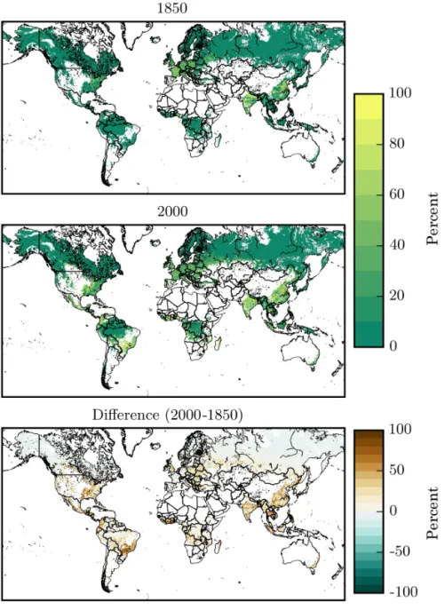
The area converted to agricultural land, defined as the sum of cropland and pasture, and that coincides with land that would otherwise be forested is calculated to determine the areal extent of deforestation, as well as reforestation, over 10-year time steps for each grid cell. Spatial data are con-verted to country time series using an area-weighted summa-tion according to the country boundaries data of the Food and Agriculture Organization of the United Nations (2015c). See also Fig. 4.
To downscale the regional emissions data, we make the assumption that forests in a region have the same average carbon content. Therefore, for any two countries in a region, we assume that converting 1 ha of forest into cropland in one country releases the same amount of CO2to the atmosphere as converting 1 ha of forest in the other country. The time-resolved data exhibit strong fluctuations, which do not nec-essarily coincide with fluctuations in the emissions data. One reason for this is the different methodological approaches used to create the two datasets. While the Houghton dataset models actual emissions from deforestation in detail, the method to calculate deforested area uses datasets that are of more theoretical nature. The HYDE dataset models the need for agricultural area in a region and does not represent the agricultural area that was actually present at that time. When population changes, the need for agricultural area changes with it, but the actual agricultural area changes more slowly. This is especially visible in Europe during the Second World
War. Population, and thus the need for agricultural area, de-clined rapidly, leading to afforestation in the SAGE-HYDE model. In reality, agricultural area will remain unused for some time until it is actively afforested or natural vegeta-tion returns and takes up carbon from the atmosphere. This leads to situations where the Houghton source has positive emissions, while the SAGE-HYDE calculation shows an in-crease in forest cover indicating CO2removals. This sign dis-crepancy causes problems for downscaling (e.g., instability if some countries in a region show afforestation and some de-forestation and a general problem of interpreting the shares in afforestation to calculate shares in deforestation emissions). To solve this problem, we do not use yearly shares but in-stead cumulative shares in deforestation for the whole period of 1850 to the last data year in the Houghton source in order to downscale the regional emissions to country level. This approach is also taken in Matthews et al. (2014). Details are given in Appendix B.
4.2.3 Composition of the land use CH4and N2O pathways
Figure 4.Calculating deforested areas: the two upper plots show the area potentially covered by forests (colored) and the fraction that has been cut until 1850 and 2000 according to the SAGE and HYDE datasets. The third plot shows the difference between the 1850 and 2000 deforestation and thus the area deforested or reforested between 1850 and 2000, which we use to downscale the Houghton dataset.
using the 21-year linear trend of the emissions from 1890 to 1910.
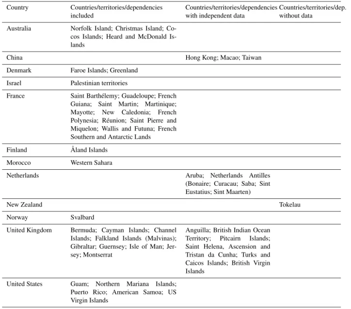
4.3 Territorial definitions, changes, and missing data
The dataset provides emissions time series for all UNFCCC member states. Some territories are associated with states but have partial independence, while other territories claim in-dependence but are not internationally recognized, or have another special status. We include the emissions from these territories in the country emissions if, and only if, the coun-try includes the emissions when reporting under the
Table 8.Territorial definitions of countries used in the dataset. The territorial definitions are based on country emissions reporting under the UNFCCC and do not imply any political judgment.
Country Countries/territories/dependencies included
Countries/territories/dependencies with independent data
Countries/territories/dep. without data
Australia Norfolk Island; Christmas Island; Co-cos Islands; Heard and McDonald Is-lands
China Hong Kong; Macao; Taiwan
Denmark Faroe Islands; Greenland
Israel Palestinian territories
France Saint Barthélemy; Guadeloupe; French Guiana; Saint Martin; Martinique; Mayotte; New Caledonia; French Polynesia; Réunion; Saint Pierre and Miquelon; Wallis and Futuna; French Southern and Antarctic Lands
Finland Åland Islands
Morocco Western Sahara
Netherlands Aruba; Netherlands Antilles
(Bonaire; Curacau; Saba; Sint Eustatius; Sint Maarten)
New Zealand Tokelau
Norway Svalbard
United Kingdom Bermuda; Cayman Islands; Channel Islands; Falkland Islands (Malvinas); Gibraltar; Guernsey; Isle of Man; Jer-sey; Montserrat
Anguilla; British Indian Ocean Territory; Pitcairn Islands; Saint Helena, Ascension and Tristan da Cunha; Turks and Caicos Islands; British Virgin Islands
United States Guam; Northern Mariana Islands; Puerto Rico; American Samoa; US Virgin Islands
the dataset despite its negligible anthropogenic greenhouse gas emissions.
As a result of the Ukraine crisis, parts of the (former) Ukrainian territory are currently claimed by both Russia and Ukraine. The UN has not recognized any changes to the Ukrainian territory, so we do not make any adjustments to the Ukrainian emissions. There are no country-reported data recent enough to be influenced by the crisis.
We use territorial accounting in this dataset, meaning that emissions that originated from a territory that is now part of country A are always counted as emissions from country A even if the territory belonged to country B in the year the emissions took place. However, we can only be as precise as the datasets we are working with. Unfortunately, many sources are not very precise with respect to the methodol-ogy used. CDIAC CO2and, to a lesser extent, FAO data are
Table 9.Uncertainties for fossil fuel and industrial CO2emissions for different country groups. All values from Andres et al. (2014).
Country class
OECD European countries outside of OECD
OPEC Developing coun-tries with stronger statistical bases (e.g., India)
Former USSR and eastern Europe
China and centrally planned Asia
Developing countries with weaker statistical bases (e.g., Mex-ico)
Uncertainty (95 % con-fidence)
4 % 6.7 % 9.4 % 12.1 % 14.8 % 17.5 % 20.2 %
know which regions were affected. However, as the land ex-change including large emitters has been small in the recent decades and emissions were relatively low before the recent decades, the influence will likely be small. CRF2014, UN-FCCC2015, and BUR2015 data are reported by countries and do not require preprocessing as we use the territorial defi-nitions of the UNFCCC reporting as a basis. For EDGAR data, the rules regarding how emissions are assigned to coun-tries in the case of territorial changes are not clear from the methodology description and we assume that territorial ac-counting is used.
For some small countries and countries that recently be-came independent, no emissions data are currently available. In this case we have to construct time series using other countries’ emissions data. Emissions data for San Marino and the Vatican are included in Italian emissions data and downscaled using population shares.20 Downscaling is per-formed on the individual sources during preprocessing (for preprocessing details, see also Appendix B). For details on the downscaling methodology see Appendix A3. Sudan and South Sudan are also downscaled from emissions of former Sudan using UN population data (UN Population Division, 2015).
5 Data availability
The dataset is available from the GFZ Data Services under doi:10.5880/PIK.2016.003 (Gütschow et al., 2016). When using this dataset or one of its updates, please cite this pa-per and the precise version of the dataset used. Please also consider citing the relevant original sources when using this dataset. Any use of this dataset should also comply with the usage restrictions of the original data sources used for this project.
6 Results
In this section we show some key results of our analysis. Details for additional countries, sectors, and gases can be explored online on our companion website
20GDP data not available.
http://www.pik-potsdam.de/primap-live/primap-hist/. Here we focus on major emitters and global emissions.
6.1 Sectoral distribution of aggregate Kyoto greenhouse gas emissions for major emitters
Globally, production and consumption of fossil fuels is re-sponsible for about two-thirds of current aggregate Kyoto greenhouse gas emissions21, which is an increase from about 50 % in 1950 and a negligible contribution in 1850. This is shown in the upper left panel of Fig. 5. Before the In-dustrial Revolution, deforestation was the major emissions source followed by agriculture. Currently, these sectors are the second- and third-largest sources. Roughly 10 % of emis-sions come from waste and industrial processes. Industrial processes increased their share in yearly emissions after 1950, while the share of waste-related emissions stayed rela-tively constant.
The sectoral profile differs strongly among countries (Fig. 5). Land use emissions reached almost zero or even negative values in the 1950s to 1970s in industrialized coun-tries (USA, EU, Japan) and a few decades later in China. For all these countries, fossil fuel use and production are by far the largest contributors to total emissions. While the indus-trialized countries have decreasing (USA, EU) or stagnating (Japan) fossil fuel emissions, China has rapidly increasing emissions. The increase in emissions from China may have slowed down in the last years, but more time is needed to say whether this is more than a temporary effect (Korsbakken et al., 2016).
India still has a large share of LULUCF emissions with no clear increase or decrease in the last two decades. Agriculture and LULUCF have similar emissions both in trends and ab-solute values, which have only recently (roughly 1990) been surpassed by the steeply increasing fossil-fuel-related emis-sions. For Brazil the largest sector is land use, followed by agriculture. Land use emissions show a decreasing trend, but total emissions do not follow this trend due to a rise in agri-cultural emissions and fossil-fuel-related emissions.
1860 1880 1900 1920 1940 1960 1980 2000 2020 0
10 20 30 40 50 60
G
t
C
O
2
e
q
World
1860 1880 1900 1920 1940 1960 1980 2000 2020 0
1 2 3 4 5 6 7 8
G
t
C
O
2
e
q
United States
1860 1880 1900 1920 1940 1960 1980 2000 2020 0
2 4 6 8 10 12 14
G
t
C
O
2
e
q
China
1860 1880 1900 1920 1940 1960 1980 2000 2020 0
1 2 3 4 5 6 7
G
t
C
O
2
e
q
European Union (EU28)
1860 1880 1900 1920 1940 1960 1980 2000 2020 0
1 2 3 4
G
t
C
O
2
e
q
India
1860 1880 1900 1920 1940 1960 1980 2000 2020 0.0
0.2
0.4
0.6
0.8
1.0
1.2
1.4
G
t
C
O
2
e
q
Japan
1860 1880 1900 1920 1940 1960 1980 2000 2020 0.0
0.5
1.0
1.5
2.0
2.5
G
t
C
O
2
e
q
Brazil
Using GWP from IPCC AR4 CAT7: Other
CAT6: Waste CAT4: Agriculture
CAT3: Solvent and other process use CAT2: Industrial processes CAT1: Total energy CAT5: LULUCF
Figure 5.Aggregate Kyoto greenhouse gas emissions by sector for major emitters and the world. Where land use emissions are negative, the stacked emissions of the other sectors start at this negative value. International shipping and aviation emissions are not included. The figure is discussed in Sect. 6.1.
Waste gives a small contribution, differing by country without a clear split between developed and developing countries. The contribution of industrial processes is larger in industrialized countries, but especially large in China.
6.2 Gas distribution of economy-wide emissions for major emitters
The contribution of individual gases and gas groups to (global warming potential weighted) economy-wide (IPCC 1996 category 0) emissions is shown in Fig. 6. It is clearly visible that CO2is by far the largest contributor,